Experimental Performance Evaluation of a Thermoacoustic Stirling Engine with a Low-Cost Arduino-Based Acquisition System

Abstract

Existing thermoacoustic dynamic measurement instrumentation is typically expensive and relies on proprietary designs, sensors, and acquisition equipment. However, this study presents a low-cost acquisition solution for sampling pressure and calculating instantaneous power measurements from a thermoacoustic engine using cost-effective sensors and control boards based on the Arduino platform. While the platform was designed for thermoacoustic engines with extra security for safe, high-speed data transfer, it could also suit other applications with similar needs. This study details the implementation of the sampling system and sensor arrangement, employing Python 3.10.2 algorithms based on the two-pressure sensor method to process and present the data. The sampling system is evaluated against a high-performance sound acquisition system. The accuracy of the low-cost system is found to be satisfactory for expected thermoacoustic experimental conditions in terms of pressure resolution and accuracy, with no data loss. These results allow for significantly increased accuracy at low cost in determining the maximum power extracted from any thermoacoustic device.

1. Introduction

Thermoacoustic engines convert heat into mechanical energy, specifically into acoustic power, which can then be utilized to produce electricity or drive other devices. Their distinctive feature lies in their minimal moving components, setting them apart from traditional thermal engines. Remarkably, the most basic configuration operates seamlessly without any moving parts: an acoustic resonator facilitates the resonance of sound waves generated within the regenerator element. The initial concept behind the development of thermoacoustic Stirling-like cycle engines (TA-SLiCEs) was initially introduced by Ceperley in 1979 [1]. He suggested that the interaction between solid components and gas resembles the thermodynamic cycle of a Stirling engine, due to the propagation of traveling waves through the regenerator. Finally, Ceperley’s concept materialized with the creation of the first TA-SLiCE in 1999 by Backhaus and Swift [2]. From that milestone, a plethora of studies were conducted, leading to the experimental development of laboratory thermoacoustic devices [3].

In a TA-SLiCE, three parts can be identified: the core, feedback, and power extraction branches. A looped tube, jet pump, compliance and inertance (feedback branch), thermal buffer tube, and regenerator, as well as its adjacent heat exchangers (core branch), mechanical resonator (piston), resistor–capacitor (RC) load, and electroacoustic transducer (power extraction branch) are the main components of these parts, which have specific roles within the engine, including, among others, the engine startup, phase shifting, acoustic power transmission to the engine core branch, and thermal relaxation or Gedeon streaming suppression [4]. In this regard, mechanical resonators can be used to estimate the total acoustic power measuring its oscillatory motion. It is important to highlight that the TA-SLiCE used in this study, depicted in Figure 1, operates effectively at 23 Hz and low pressures amplitude, with a design and fabrication that emphasize low-cost materials, as previously published [5]. This approach not only demonstrates the device’s operational feasibility but also underscores the potential for broader application through cost-effective manufacturing strategies.

To provide valuable information about the engine’s performance, the acoustic power is a critical parameter to consider [4]:

$$\dot{E}=\frac{1}{2}\left|p\right|\left|U\right|\cos {\varnothing }_{pU},$$

(1)

where ${\varnothing }_{pU}$ is the phase shift between pressure amplitude $p$ and volumetric velocity $U$.

By evaluating the acoustic power, inefficiencies in the engine’s design can be identified, leading to more focused improvements and optimizations [5]. However, measuring the phase difference between acoustic pressure and particle velocity in a thermoacoustic resonator is challenging. The standing wave ratio is very high in such resonators, and the working frequencies are resonance frequencies. The angle ${\varnothing }_{pU}$ is usually close to π/2; this makes $\cos {\varnothing }_{pU}$ difficult to determine with sufficient precision unless complex and costly measuring devices are used (laser-based instruments [6] or lock-in amplifiers [7]).

Acoustic power flow in thermoacoustic devices can be directly measured through methodologies such as the one developed by Hofler [8], which involves the use of a high-intensity acoustic driver apparatus to measure the acoustic power delivered to the resonator. Additionally, techniques like hot-wire anemometry (HWA), laser Doppler anemometry (LDA), and particle image velocimetry (PIV) can also be employed. However, all these require the use of specialized and complicated instrumentation for velocity measurements in thermoacoustic systems [6].

An established indirect method of estimating acoustic power is based on the two-pressure sensor method. Based on the literature review [9,10], it can be concluded that the two-pressure sensor method using the RC load technique, described by Fusco et al. [11], is effective for measuring local acoustic power in thermoacoustic engines. Therefore, the two-pressure sensor approach was used in this study to enable instantaneous acoustic power calculation. This method is explained in Section 2.2.

It should be noted that most of the published works in thermoacoustics using low-cost systems have focused on quasi-static acquisition, i.e., for temperature sampling [12,13,14]. This limitation may be due to the fact that low-cost sensors and instrumentation often have lower sensitivity and accuracy compared to their higher-cost counterparts. There is a need to extend their applications to dynamic measurements to facilitate the exploration of the potential of thermoacoustic engines for researchers and industries.

It is noteworthy that, according to the literature, the use of low-cost data acquisition systems in thermoacoustics for dynamic acquisition is still limited [15]. The scarce studies that have been published to date have not validated their results against robust professional counterparts [16,17,18]. In this regard, this paper is focused on comparing the performance and reliability of economic data acquisition systems against established professional systems applied to thermoacoustic devices.

The proposed low-cost system consists of affordable technology for both the monitoring system (utilizing low-cost absolute pressure sensors) as well as data acquisition (employing Arduino-based systems). Despite its cost-effectiveness, the system ensures the validation of accuracy and functionality through the integration of a professional-grade reference system. Building upon the promising results from previous studies [15] that utilized pressure sensors with Arduino for its robustness [19], it is expected that the developed system will demonstrate effectiveness in measuring instantaneous acoustic power in thermoacoustic devices. Furthermore, the cost-effective sensor implementation and data acquisition used in the TA-SLiCE can be readily applied to other thermoacoustic devices and other areas of acoustics, thereby broadening the scope of application, and generating increased interest.

This article is distributed as follows: Section 2 describes the experimental setup of the low-cost thermoacoustic engine and data acquisition system. Section 3 presents the results and the discussion of the simultaneous low- and high-cost data acquisition, and Section 4 summarizes the conclusions of this paper.

2. Materials and Methods

2.1. Low-Cost TA-SLiCE

The investigation was conducted utilizing an experimental TA-SLiCE. This engine was designed and manufactured in accordance with the guidelines outlined in [5]. This section introduces its design modifications, with a focus on optimizing the components to achieve a main objective: making TA-SLiCEs easily reproducible for low-power applications. The configuration of the TA-SLiCE investigated in [5] and in the present study is similar to the 3D model developed using computer-aided three-dimensional interactive application software (CATIA V5 6R2019, Dassault Systèmes, Ile-de-France, France) depicted in Figure 2. The regenerator is a screen made of stainless steel with 40 openings per inch and a 0.44 mm wire diameter.

The TA-SLiCE illustrated in Figure 2 was firstly modelled using the Design Environment for Low-Amplitude Thermoacoustic Energy Conversion DeltaEC Software (DeltaEC Release 6.4b2.7, Los Alamos National Laboratory, Los Alamos, NM, USA) [20], which relies on Rott’s linear theory [4], to search for the optimal design operating at 23 Hz with air at atmospheric pressure and keeping the heat source and heat sink temperatures at around 641 K and 296 K, respectively. DeltaEC offers valuable insights into acoustic field properties, assuming a linear acoustic approach with features like plane waves, laminar flow, and no streaming. These simulation details are fully explained in [5]. For the TA-SLiCE used in this paper, some design modifications were implemented with respect to previous versions:

• Manufacture using acrylonitrile–butadiene–styrene (ABS) and sealing with acetone.

Three-dimensional fused deposition modeling (FDM) was used to manufacture the components of the TA-SLiCE. This provides high flexibility in constructing all its elements, enabling quick evaluation of each design regardless of complexity. The choice of ABS over the commonly used polylactic acid (PLA) is not due to the former’s mechanical properties but its superior post-processing for achieving the necessary seal for this application. The key reason is ABS’s easier post-treatment compared to PLA, which, to ensure sealing, requires specific chemicals like tetrahydrofuran (THF), ethyl acetate, butanone, dichloromethane (DCM), chloroform, etc. These industrial solvents can be hazardous if not handled and used properly. In contrast, applying a layer of acetone for ABS post-processing is sufficient to ensure complete sealing after the compounds react. This approach also offers the flexibility to print sectioned parts that can later be welded together using acetone, significantly easing the printing process. This is particularly beneficial for achieving better layer deposition in components requiring 100% infill.

• Incorporation of nitrile–butadiene–rubber (NBR) O-rings in the element connections in order to isolate cavities and avoid fluid leaks.

The addition of O-ring grooves facilitates the easy assembly and disassembly of the engine. Previously, the use of sealing paste made this process challenging. NBR O-rings were incorporated to prevent air leaks through the Pyrex thermal buffer tube (TBT) and cooling jackets, and at the ends of the cooling jackets to prevent water from the cooling system from penetrating into the engine. This design consideration enhances both the operational efficiency and maintenance convenience of the engine, ensuring airtight seals where necessary while allowing for straightforward component adjustments or replacements. The compression needed for effective sealing is provided by mechanical joints using screws and nuts located in the refrigerators themselves, along with aluminum compression rings. These components work together to apply the necessary force to ensure a tight seal, preventing any leakage and maintaining the integrity of the system.

• Incorporation of aluminum inserts and use of standard hydraulic connectors.

Metal inserts were used, as shown in Figure 3, to avoid threading directly into the 3D-printed piece, a process that otherwise requires threading taps to be applied afterwards. This method has limitations both in terms of sealing and the number of times the connections can be disassembled. Therefore, incorporating brass aluminum inserts using a heat source enables the creation of leak-proof and securely fastened connections in the base piece. This approach simplifies the use of standardized threaded hydraulic connectors (M5) for all connections to sensors and the cooling ports themselves.

• Adaptive inertance.

Figure 4a shows how in earlier TA-SLiCE versions, the feedback branch inertance was built directly into the 3D-printed part, including a fixed elbow. Figure 4b shows the latest design for this study, introducing adjustable inertance by connecting tubes of different lengths to an elbow with an adjustable angle. Thus, the design becomes more flexible and allows for adjusting the system’s dynamics more precisely by modifying the path of the feedback branch, making the setup a more versatile tool for experimental investigations.

• Simplification of RC loading

To measure the output acoustic power of the constructed TA-SLiCE, the variable RC load shown in Figure 5 is connected to the power extraction branch. The valve acts as the variable resistance, and the tank positioned over the valve serves as the compliance. This configuration not only allows for the precise measurement of acoustic power using the two-pressure sensor method and RC load technique, but also enables the achievement of maximum power dissipation by operating the load with the valve open just before the point at which the piston ceases to move.

• Change in thermal power input system.

The last modification involved replacing the alcohol burner, previously used as the source of thermal power input, with two 50 W bulbs. This change led to an enhancement and an increase in the input power, as well as greater precision in quantifying the incoming heat.

These adjustments are aimed at enhancing the system’s functionality, increasing its reliability, and simplifying its replication. Further details about the design of the TA-SLiCE can be found in the work by Iniesta et al. [5].

2.2. RC Load Method

In this section, a brief overview of the physical background behind the employed method for acoustic power measurement is provided. It is crucial to introduce the concept of lumped-element approximation, initially proposed by Ceperley [1], which stablishes an analogy between the acoustic impedance ($Z_a$) and the impedance of an electrical circuit ($Z$) [4]:

$$Z_a=\frac{p_1}{U_1}=R_a+j\left(\omega L_a-\frac{1}{\omega C_a}\right) \leftrightarrow Z=\frac{V_1}{I_1}$$

(2)

where $R_a$ is a resistive acoustic load (resistance), $L_a$ is an inductive acoustic load (inertance), $C_a$ is a capacitive acoustic load (compliance), and $\omega$ is the acoustic frequency. $p_1$ and $U_1$ are the pressure wave amplitude and the volumetric flow rate, respectively. $V_1$ and $I_1$ are the electric AC voltage and the electric AC current, correspondingly.

It is interesting to note that the compliance introduces a positive phase shift of 90° between $\left|p_1\right|$ and $\left|U_1\right|$, meaning it acts as a capacitive load so that the flow advances 90° in relation to the pressure. Resistance, however, does not cause a phase change between $\left|p_1\right|$ and $\left|U_1\right|$. Accordingly, in Equation (2), the compliance is purely imaginary, whereas the resistance is purely real.

Assuming the short duct length approximation, any compliance can be written [21]:

$$C=\frac{V}{\gamma P_m}$$

(3)

where V, $P_m$, and $\gamma$ are the volume of the compliance, mean pressure, and specific heat ratio.

A variable RC acoustic load is connected to the power extraction branch of the TA-SLiCE under study, as shown in Figure 6, to indirectly measure the volumetric flow rate through the resistance.

Assuming simple harmonic sound at angular velocity $\omega$:

$$U_1=j\omega C{P}_C=j\omega \frac{V}{\gamma P_m} P_C$$

(4)

Hence, the dissipated acoustic power at the resistance is determined using the RC load method described by Fusco et al. [11]. A variable RC load can be constructed by connecting a small volume tank to the mechanical resonator of the power extraction branch through a needle valve, shown in Figure 4 and Figure 5. This method requires little equipment, two pressure sensors; one of them is placed close to the inlet of the needle valve, while another is installed inside the tank. By measuring the acoustic signals from these two sensors, it is possible to determine the instantaneous amount of acoustic power that is lost due to dissipation in the load:

$${\dot{E}}_{RC}=\frac{1}{2}\frac{\omega V}{\gamma P_m}Im\left(P_E{\tilde{P}}_C\right)=\frac{1}{2}\frac{\omega V}{\gamma P_m}\left|P_E\right|\left|P_C\right|sin{\theta }_{EC},$$

(5)

The acoustic power dissipated in the RC load is determined as the time-averaged product of the volumetric flow rate through the valve and the two pressures ($P_E \mathrm{and} P_C$) across the valve. $V$, $P_m$, and $\gamma$ are volume of the tank, mean pressure, and specific heat ratio. ${\theta }_{EC}$ is the phase shift in radians between the pressure measured at the mechanical resonator, $P_E$, and the pressure measured at the volume tank, $P_C$. This algebraic expression represents a revision and simplification of previous models and expressions from the two-pressure sensor method by analyzing pressure measurements at two points a specific distance apart at the power extraction location. This broadly used method, which yields a refined expression of the power available for extraction in thermoacoustic devices, only needs to measure the two pressure signals $P_C$ and $P_E$ (amplitude, phase, and acoustic frequency $\omega$).

2.3. Cost-Effective Data Acquisition System

The present research is aimed at developing a robust, cost-effective acquisition system for thermoacoustic experimentation. The effectiveness of data acquisition systems in thermoacoustics is limited by the fact that the engines’ dynamics cannot be fully analyzed without a reliable data acquisition system.

This section describes the proposed data acquisition system to calculate the acoustic power of the TA-SLiCE. The system is designed to be both precise and cost-effective, following the approach of previous research [15]. The Arduino-based system, developed and validated in earlier work, was adapted and improved to meet new requirements. The Arduino board captures analog input each firmware cycle and transmits it to the microcomputer via USB as a byte sequence, following the serial communication protocol detailed in [19]. The performance of the proposed system is compared with a high-cost Brüel and Kjaer (B&K) system, using the same type of pressure sensor. The B&K Photon+ system, designed for real-time measurements of vibrations and acoustics, features a high-performance digital signal processor (DSP) and is considered an exact reference for this investigation. All data were stored in comma-separated value (CSV) files for subsequent processing on a Raspberry Pi 3B+, which served as a PC.

The following describes and justifies the type of sensors used and also the rest of the laboratory equipment to measure and record the raw data obtained by the sensors for further processing and interpretation. Thus, the acquisition system consists of a pressure sensor array, an electronic board that reads the values provided by the sensors, and the algorithms, based on the two-pressure sensor method, that allow for interpreting the sensors’ data and calculating the acoustic power.

2.3.1. Pressure Sensors

As previously mentioned, the engine is designed to operate at a 23 Hz frequency, which is a critical factor in selecting the appropriate measurement instruments. Once the system achieves stability and oscillates consistently around the resonance frequency, data acquisition and, consequently, recording of the engine’s operational cycles begin.

Before specifying the placement of each sensor, it is essential to clarify the concept of acoustic power, crucial for understanding the monitoring points within the system. Figure 7 illustrates the acoustic power generated during the Stirling cycle at the engine’s core (${\dot{E}}_{core}$), which is distributed in two main pathways: the transit through the feedback branch and the instantaneous work exerted on the power extraction branch.

The feedback branch absorbs power (${\dot{E}}_{feedback}$), which is employed for feedback purposes, enabling the traveling wave to return to its initial starting point at the beginning of the duty cycle. The power diverted to the power extraction branch has two contributions (${\dot{E}}_{junction}+{\dot{E}}_{RC})$. The power that can be measured at the RC load is considered the effective power (${\dot{E}}_{RC}$), which can be extracted and used. This paper specifically analyzes the effective power. The amount of acoustic power dissipated in the RC load varies depending on the position of the valve regulating the flow resistance to the acoustic cavity, while the remainder is used to drive the resonating piston (${\dot{E}}_{junction}$). This action must overcome friction within the cylinder to achieve displacement. To achieve maximum power dissipation in the load, the system operates with the valve open just before the point at which the piston ceases to move. It is important to point out that the RC load was installed in the TA-SLICE system specifically for the experimental evaluation of the power output. In normal conditions, i.e., if the TA-SLICE were functioning as an energy converter (from heat to mechanical power), the RC load would be fully closed, or simply taken apart.

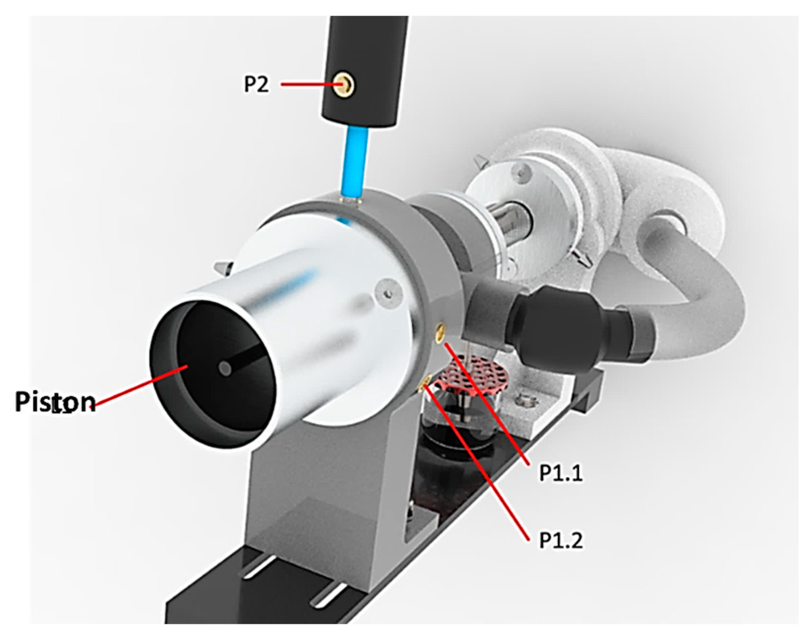
Figure 8 illustrates the three low-cost Farnell (P1.1, P1.2, and P2) piezoresistive absolute pressure sensors (MPX5100AP) used to measure the two pressure oscillations in the power extraction branch of the mechanical resonator. For double validation of the results, sensors P1.1 and P1.2 are positioned near the inlet of the needle valve, while sensor P2 is located in the tank. The RC load pressure is monitored with a single low-cost sensor, as double validation in this region would be redundant. The data from the other sensors provide sufficient conditions to extrapolate behavior to this region.

At this stage, it is relevant to remember that the engine oscillates around $23 \mathrm{Hz}$. Consequently, the sensor must capture values at a minimum sampling frequency of $F_s\ge 46 \mathrm{Hz}$ to prevent aliasing, thereby ensuring that the acquisition frequency is at least double the original sampled frequency. In this work, the sampling frequency was set at $F_s=600 \mathrm{Hz}$, significantly exceeding the Nyquist–Shannon sampling requirement, thereby adequately fulfilling this criterion.

The P1.1, P1.2, and P2 sensors are supplied with 5 V and deliver a continuous analog voltage output ranging from 0 to 5 volts, corresponding to a pressure range of 0 to 110 kilopascals (kPa) at a response time of 0.001 s and a $\pm 2.5\%$ accuracy of the full-scale span [22]. Figure 9 offers a comprehensive depiction of the MPX5100AP sensor and its pressure-to-voltage transfer function within the designated range.

In the present research, the atmospheric pressure within which the sensor operates ranges from 80 to 100 kPa. The signals to be measured are sinusoidal in nature, reflecting the cyclic operation of the engine, with a peak-to-peak amplitude ranging from 5 to 10 kPa. This makes the MPX5100AP sensor adequate for this measurement requirements.

2.3.2. Acquisition Board and Firmware

In accordance with the low-cost framework of this study, the chosen data acquisition board was an Arduino Mega 2560 R3 (Arduino Mega 2560 Rev3, Arduino, Turin, Italy). This board is notably prevalent and operates on the 8-bit, 16 MHz ATmega2560 microcontroller, featuring 16 analog-to-digital converter (ADC) inputs that directly operate at 5 V, thus eliminating the need for any intermediary interface with the pressure sensors. Moreover, the ADC resolution is adjustable from 10 to 12 bits, ensuring accurate reconstruction of the sinusoidal signals detected by the pressure sensors. This configuration aligns with the research’s aim for cost-efficiency while maintaining the integrity and precision of data collection.

This acquisition board is used to read the sensor signals and pass the values to the computer where they will be processed and analyzed. The connection with the pressure sensors is made directly through the ADC ports, which translate the sensors’ voltage output into a digital number stored in the microcontroller’s memory. Figure 10 illustrates the wiring diagram of the data acquisition systems specifically employed for this work. On the computer side, the communication is performed with a universal serial bus (USB) connection over a serial protocol. Arduino firmware provides its own serial function to send and receive data in a reliable manner. However, the transmission speed is low for high- or medium-frequency applications. In order to obtain higher speeds in data transfer, an ad-hoc communication protocol was developed and tested in a previous work. Such protocol manages data at byte level and applies different framing techniques to ensure data compliance, achieving frequencies of about 3 kHz for a single sensor with no data losses. In [19], a detailed description of the protocol and the statistic evaluation of its speed and robustness can be found.

2.3.3. Signal Processing Algorithms

This section describes the strategy to achieve the desired acoustic power, as outlined in the theoretical method detailed in Section 2.2. Alongside scripts that enhance the Arduino’s data acquisition frequency, this algorithm forms the basis of an immediate platform for measuring data from thermoacoustic devices. It is important to note that in this section, the approach adopted to address the unexpected time error behavior identified in preceding studies is detailed [15]; this involves adjusting the internal quantization reference of Arduino. Specifically, the ATMega2560 converter, which typically quantizes the continuous input signal using a default 5 V output reference, allocates the total resolution bits across a 0–5 V range. This default setting was modified through the acquisition code loaded onto the board by employing the analogReference function.

In the operation of ADC converters, the input signal intended for quantification is successively compared with a reference voltage. When the input signal matches the reference voltage, both precision and resolution are optimized. However, if the input value is significantly lower than the reference voltage, a substantial portion of potential comparisons and value assignments is not utilized effectively. This underutilization leads to a consequent loss in resolution, as the system is unable to fully capitalize on its comparative range and resolution capacity. To address this limitation, the function analogReference (EXTERNAL) was employed to modulate the reference voltage. This adjustment allowed for the reference voltage to match the voltage input received at the AREF pin, which was controlled via a potentiometer. By varying the input voltage in this manner, an enhancement in resolution was achieved, enabling the ADC system to better utilize its full range of comparative and resolution capabilities for enhancing resolution.

In the initial stage of the signal processing workflow, R software (R Release 4.1.2, R Foundation for Statistical Computing, Vienna, Austria) and its integrated development environment, RStudio (RStudio Release 4.1.2, Posit Software, PBC, Boston, MA, USA) (both open-source), were employed to manage raw data. The objective was to produce a refined dataset for further analysis. An automated system was set up to systematically read all files from their storage locations, organize them, and process them according to a pre-established template. This automated preprocessing significantly reduces the time required for post-processing by standardizing the input data. Following the preparation of data, some scripts were developed in Python (Python Release 3.10.2, Python Software Foundation, Beaverton, OR, USA) using numpy, scipy, pylab, pandas, matplotlib, tabulate, and mpld3 libraries to calculate the power output of the engine under different experimental conditions, based on the input data files. The operational approach remained consistent throughout, requiring the implementation of an algorithm that fits the data within each time window to a sinusoidal function, according to Equation (6), of a harmonic wave:

$$y\left(t\right)=Asin\left(\omega t+\phi \right)+c$$

(6)

The fitting process was conducted using fast Fourier transform (FFT), enabling the extraction of the fundamental and characteristic parameters of the wave: amplitude ($A$), frequency ($f=\frac{\omega }{2\pi }$), phase ($\phi$), and offset ($c$). The fitting of the input data arrays to a sine function was performed using the ‘$fit\_sin\left(t, y\right)$’ function in Python. The algorithm includes several steps that clearly outline how the sinusoidal parameters are derived from the input data:

• Start
• Generate Arrays
  • Generate one array from the time data column.
  • Generate another array from the measurement records.
• Compute Sample Frequencies
  • Use fft.freq function from the numpy library to obtain the sample frequencies of the discrete Fourier transform.
• Frequency Centers
  • Store frequency centers in array f. Frequency is expressed in cycles per unit of sample spacing (zero at the beginning).
  • Example: if sample spacing is in seconds, frequency unit is cycles/second.
• Calculate DFT
  • Calculate the one-dimensional discrete Fourier transform (Fyy).
  • Use the fast Fourier transform (FFT) algorithm to compute DFT of n points.
• Find Maximum Frequency
  • Use numpy.argmax() to find the index with the maximum value in the Fyy array.
  • Extract the corresponding frequency value from the array f.
• Calculate Amplitude
  • Determine the standard deviation of all signal records.
  • Multiply by the square root of 2 to find the amplitude.
• Determine Phase
  • Use scipy.optimize.curve_fit to determine the phase.
• Calculate Offset
  • Calculate the mean value of the data to find the offset.
• Define Sinusoidal Function
  • Define an internal function to represent the sinusoidal function based on extracted parameters.
  • Follow the equation: y(t) = A⋅numpy.sin(wt + p)+cy(t) = A⋅numpy.sin(wt + p) + c
• End

Consequently, the Arduino code is loaded, and the Python code is executed in the terminal for the measurement of output acoustic power.

As discussed at the beginning of Section 2.3, simultaneous data acquisition is crucial for validating the proposed system through a comparison against the high-cost B&K data acquisition system (DAQ) using the same pressure sensors. To ensure that measurements from both systems start at the same moment for the sensors being evaluated ($\mathrm{P}1.1$ linked to the B&K DAQ and P1.2 linked to the presented low-cost system), a trigger mechanism is implemented that generates a voltage on a digital pin of the Arduino board. This pin is connected to one of the channels of the B&K, which is configured to start measurements when a drop in potential is detected at its input. As a result, when the Arduino code is loaded and the Python code is executed in the terminal, both acquisition systems automatically begin measuring at the same time for different sensors (that monitor points in close proximity). Additionally, a LED diode was installed to indicate when the code is running, and both systems start logging data into a discrete time series in a $‘.dat’$ file.

3. Results and Discussion

This section presents the results obtained following the comprehensive post-processing methodology described earlier. In addition, the results are compared with a high-cost system to validate the effectiveness of the introduced low-cost system.

3.1. Using the Low-Cost Acquisition System to Calculate Acoustic Power

Figure 11 illustrates the clear and low-noise signal outputs recorded by P1.2 and P2 sensors over a 6 s interval, without any requirement for further smoothing or processing.

The sensors’ performance, as seen in Figure 11, confirms their appropriateness for capturing high-quality acoustic data. The enhancement in data acquisition frequency and the systematic preprocessing of the raw data, as established and described in Section 2.3.3, enabled direct plotting of highly resolved signals. The precise data handling and the ability to maintain signal integrity, especially near the sensors’ full scale, are demonstrated, showcasing significant improvements over prior methodologies that struggled with lower amplitude and higher noise levels in different testing setups [15].

Additionally, the sinusoidal fitting process detailed in Section 2.3.3 was executed to obtain the results of critical wave parameters accurately and automatically for $\mathrm{P}1.2$ and $\mathrm{P}2$ sensors, shown in Figure 12.

In the merged signals graph of the P1.2 and P2 pressure sensors presented in Figure 12, an interval of 0.16 s displays a phase shift close to 90° between both signals. This behavior aligns with the theoretical principles of the RC load method, constituting the initial validation point for the system.

Based on the results, and in accordance with Equation (5), it is possible to calculate the power from the available pressure measurements using the RC load method. This approach enables the determination of the instantaneous amount of acoustic power lost due to dissipation in the load. As a result, the maximum acoustic power obtained on the RC load was $\dot{E}\left(load\right)=112.494 \mathrm{mW}$.

The illustrated results clearly show that the proposed low-cost acquisition system, along with the detailed algorithms, enabled precise and consistent measurements of output acoustic power in the load, thereby highlighting the effectiveness of the data acquisition system in the experimental setups, including those in thermoacoustic devices.

3.2. Validation of the Low-Cost Acquisition System in a Thermoacoustic Engine

This section details the quality criterion established for validating the performance of the Arduino low-cost system against the B&K system. Both the Arduino and B&K systems have high input impedance (Arduino: ${10}^7 \mathsf{\Omega }$, B&K: ${10}^6 \mathsf{\Omega }$), ensuring accurate measurements despite parallel connection. Notably, while the B&K system is significantly more expensive, the Arduino provides a cost-effective alternative without compromising accuracy.

The validation process involves analyzing the resultant parameters from each P1.1 and P1.2 sensor pressure signal independently and calculating the percentage of absolute error:

$$Error=\left[\frac{M_{Brüel}-M_{Arduino}}{M_{Brüel}}\right]\times 100,$$

(7)

considering $M_{Brüel}$ as the measurements from the high-cost system (the real and hence more accurate values) and $M_{Arduino}$ as the measurements from the low-cost acquisition system presented in this paper. Figure 13 presents four measurements corresponding with four different pressure and frequency values. This was achieved by modifying the position of the valve.

The comparison between the Arduino and B&K systems revealed discrepancies in pressure amplitude and frequency measurements that were typically less than 1.6% and 0.3% of reading, respectively. These results clearly demonstrate and confirm the good performance of the low-cost system.

4. Conclusions

This study successfully demonstrated the feasibility and efficacy of a low-cost data acquisition system for measuring instantaneous acoustic power in thermoacoustic engines, with particular emphasis on the data acquisition process. While previous studies with low-cost systems focused on low-frequency acquisition, mainly for temperature sampling, this study demonstrates the feasibility of extending these applications to dynamic acquisition. The system, based on Arduino and employing cost-effective pressure sensors, was thoroughly tested and compared against a high-cost, professional data acquisition system. The low-cost system demonstrated satisfactory performance in terms of pressure resolution and timing accuracy, with no data loss during single sensor measurement, confirming its utility for experimental setups in thermoacoustics. In addition, this paper provides valuable details for the design and fabrication of the thermoacoustic engine used in this study and how the expected output power of such an engine could be measured using the two-pressure and RC load techniques.

The proposed system facilitates the acquisition, monitoring, and storage of acoustic wave power data in real time. Moreover, this study validates the low-cost system’s capability to accurately capture and process dynamic signals. Comparisons with a high-performance B&K system demonstrate that the low-cost system achieves satisfactory accuracy with an error margin less than 2% for pressure amplitude and frequency measurements. This level of accuracy is adequate for most experimental setups in thermoacoustics, where precise, yet budget-friendly solutions are required. Thus, the system provides a valuable tool for the study of complex phenomena in thermoacoustic engines, such as phase relationships and power flows, which are essential for improving the efficiency and understanding of these devices.

Although tailored for thermoacoustic engines, the flexibility of the system’s design and the general approach of using Python algorithms for signal processing suggest that it can be adapted to other applications for dynamic measurements. This could include studies on acoustic properties of materials, noise analysis, and other engineering applications where cost-effective data acquisition is required.