Inferences on the Generalized Inverted Exponential Distribution in Constant Stress Partially Accelerated Life Tests Using Generally Progressively Type-II Censored Samples

Abstract

This article discusses different methods for estimating the shape and scale parameters of the generalized inverted exponential distribution (GIED) and the acceleration factor in constant stress partially accelerated life test (CSPALT) with general progressively Type-II censored samples. We obtain the maximum likelihood estimates for the three parameters and calculate correlated approximate confidence intervals. Bayesian point estimates and credible intervals are also determined using the importance sampling method. Monte-Carlo simulation studies are conducted to demonstrate and compare the effectiveness of the proposed parameter estimation techniques. Additionally, a real-life dataset is examined to highlight the practical utility of these methodologies. Our findings indicate that the GIED provides an appropriate and flexible model for the real lifetime data, and the Bayesian approach offers better estimation than classical methods under most scenarios, in terms of using generally progressively Type-II censored samples under CSPALT.

1. Introduction

The exponential distribution has been repeatedly used to represent lifetime data in life testing trials or for reliability research. The reason for this is because it possesses a constant hazard rate function that can depict the attributes of the units being tested. However, the exponential distribution may not be flexible enough in more complex situations. Ref. [1] discussed another alternative called the inverted exponential distribution (IED) and calculated the estimates of the parameters of IED. In [2], the Bayesian method was used for estimating the risk function and parameters of IED. As an additional technique to improve the IED, the generalized inverted exponential distribution (GIED) was suggested by [3]. GIED has an additional shape parameter, making it more flexible and suitable for various applications.

Consider a random variable X conforming to GIED. It is characterized by its probability density function (PDF), cumulative distribution function (CDF), survival function (SF), and hazard rate function (HRF) shown below:

$$\begin{array}{cc}\hfill f_1\left(x\right)=& \alpha \lambda x^{-2}{e}^{-\frac{\lambda }{x}}{\left(1-e^{-\frac{\lambda }{x}}\right)}^{\alpha -1},x>0;\alpha ,\lambda >0,\hfill \\ \hfill F_1\left(x\right)=& 1-{\left(1-e^{-\frac{\lambda }{x}}\right)}^{\alpha },x>0;\alpha ,\lambda >0,\hfill \\ \hfill S_1\left(x\right)=& {\left(1-e^{-\frac{\lambda }{x}}\right)}^{\alpha },x>0;\alpha ,\lambda >0,\hfill \\ \hfill H_1\left(x\right)=& \alpha \lambda x^{-2}{e}^{-\frac{\lambda }{x}}{\left(1-e^{-\frac{\lambda }{x}}\right)}^{-1},x>0;\alpha ,\lambda >0,\hfill \end{array}$$

(1)

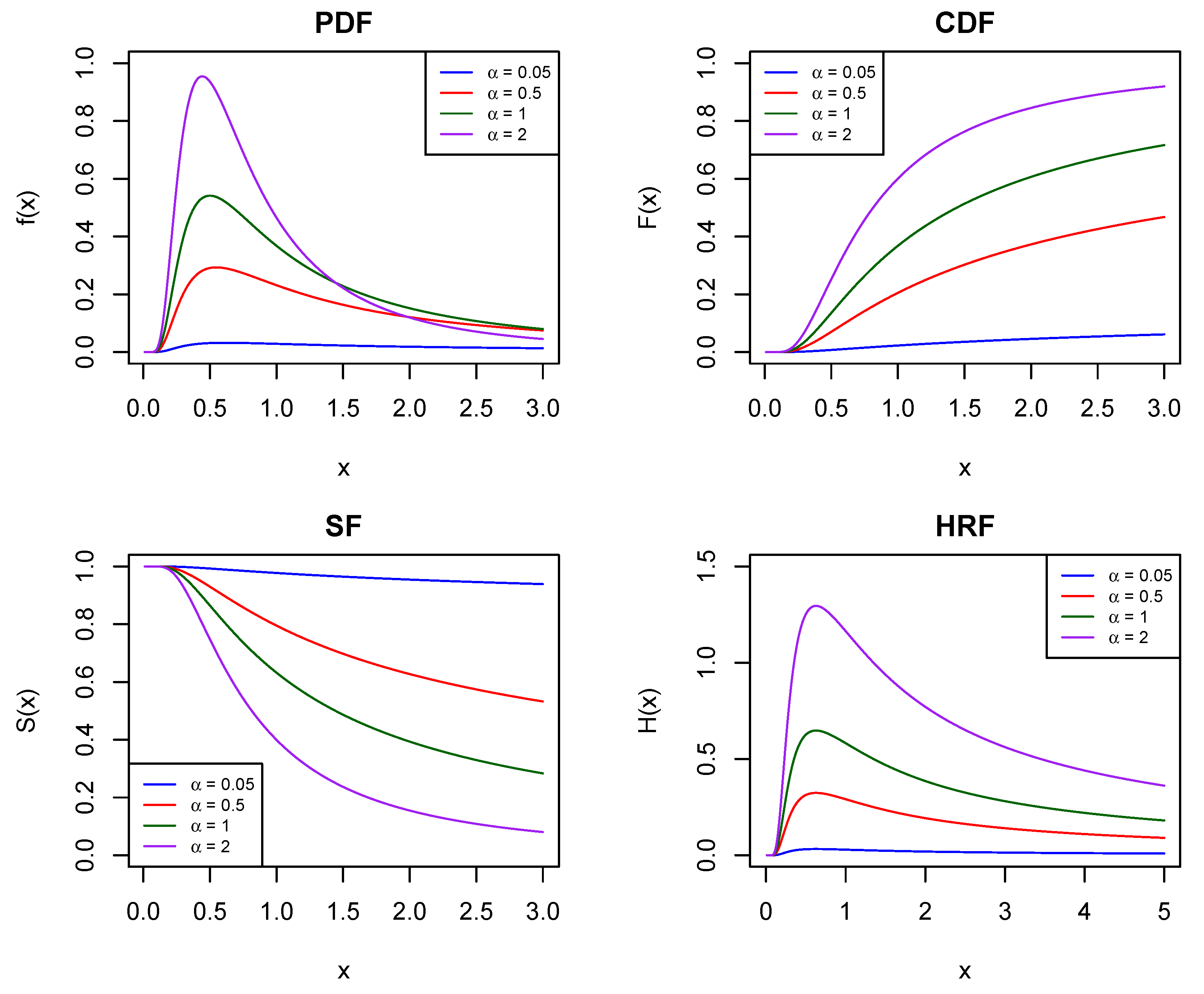
where $\lambda ,\alpha >0$ are called the scale and shape parameter separately. It is worth noting that when $\alpha =1$, GIED is simplified to a special case: IED. Figure 1 displays various curves illustrating PDF, CDF, SF, and HRF of GIED, featuring $\lambda =1$ (the scale parameter) across different scenarios featuring distinct values for $\alpha$, namely the shape parameter. Compared with the exponential distribution with a constant hazard rate function, GIED features a versatile hazard rate function, the value of which varies according to the parameter $\alpha$, see [3]. Different works were presented on GIED, ref. [4] considered the maximum likelihood estimation of the two parameters involved and derived reliability and failure rate functions under progressively type II censoring scheme in view of time cost. Ref. [5] obtained estimation of the parameters of GIED from both classical and Bayesian views and discussed a method of obtaining the optimum hybrid censoring scheme. Ref. [6] proposed a two-stage group acceptance sampling plan for generalized inverted exponential distribution under truncated life test.

As technology advances, modern products are becoming more reliable and have longer lifetimes. This makes it difficult for experimenters to conduct tests that accurately determine the actual lifetime of the products within a reasonable time frame. To solve this issue, accelerated life test (ALT) has been devised as an option. These tests subject the units to more extreme conditions than normal, such as higher pressure, temperature, voltage, etc., in order to expedite failure. There are various models under accelerated life tests (ALTs) according to different ways how the stress is exerted. In a constant stress model, all the products endure an unvarying stress level until the experiment concludes or all the units fail. This type of model has been thoroughly investigated by numerous scholars. For example, ref. [7] developed a constant stress ALT model for data that follows the Lindley distribution, while ref. [8] developed a constant stress model for exponential and Weibull data to predict how much time could the products remain. In contrast, with a step stress model, the stress level changes at specific times or when a designated number of units fail. As a result, the stress on all the products increases gradually according to some type of rule. Many authors have extensively researched the step stress models. For recent literature on this topic, ref. [9] provided a procedure of determining optimal designs of simple step-stress accelerated life tests. Ref. [10] considered a simple step-stress life test in the presence of exponentially distributed competing risks with Type-II censored data. Ref. [11] considered a simple step-stress model based on a complete sample that follows the Weibull distribution and derived the maximum likelihood estimation and Bayesian estimation. Ref. [12] provided a comprehensive exploration of accelerated life models and discussed the theoretical foundations of the models.

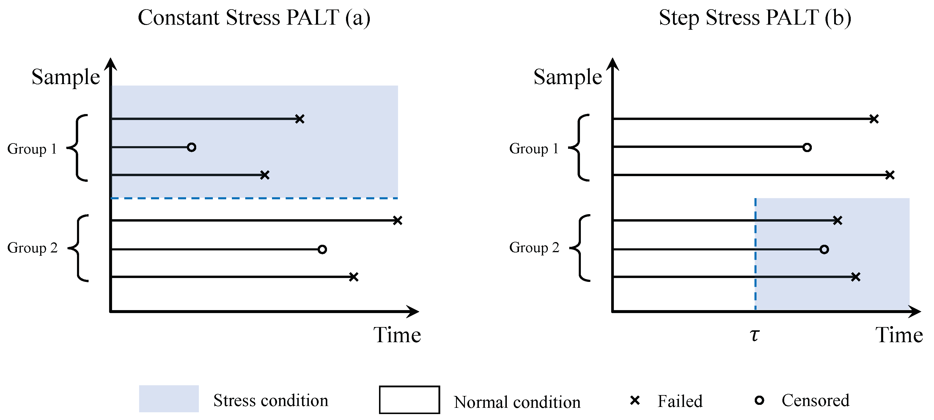
To better extrapolate the lifetime under normal use conditions, partially accelerated life test (PALT) was developed. It divides all products into groups and test each in normal and accelerated environments. Two sorts of prevalent PALTs are known as the constant stress partially accelerated life tests (CSPALTs) and the step stress partially accelerated life tests (SSPALTs). CSPALTs set different groups of units under use and stress condition respectively. By comparison, SSPALTs start with normal conditions and switch to accelerated conditions if the unit does not cease to function before a prefixed point in time $\tau$. The specific illustration of the differences between the two PALTs are displayed in Figure 2. Many researchers have studied PALTs, ref. [13] considered the CSPALTs with type-I censoring under Weibull distribution and minimized the asymptotic variance of the maximum likelihood estimators. Ref. [14] developed a SSPALT under adaptive type-II progressive hybrid censoring scheme with test items following the inverted Lomax distribution and obtained the maximum likelihood estimation of the model parameters.

Censoring is another strategy of important use that can significantly reduce the test time and cost. It involves knowing only parts of all the units’ exact failure times while the other units are removed or lost from the experiment before they fail. This helps experimenters save time and reduce costs. There exist numerous censoring schemes (CSs), with the prevalent ones being Type-I and Type-II censoring. For the former, the experiment concludes after a predetermined duration, and for the latter, the test stops upon a specific number of unit failures. Moreover, a broader, more adaptable, and efficient approach known as progressive Type-II censoring was introduced into practical problems by [15]. In this censoring scheme (CS), suppose there are n units undergoing a lifetime test, and $R=(R_1,R_2,\cdots ,R_m)$ represents some predetermined CS. Immediately following the initial failure, a random elimination of $R_1$ units is made from the $n-1$ units which are still functioning. Then $R_2$ units are withdrawn from those $n-2-R_1$ still working ones. This process is repeated until the mth failure takes place, at which instant the experimenter eliminates all of the $n-m-R_1-R_2-\cdots -R_{m-1}$ remaining units, then this test concludes. Researchers have done a lot of work on these CSs. In [16], CSPALTs using adaptive progressively Type I censored samples are taken into account and the estimation of model parameters are derived using maximum likelihood, maximum product and Bayesian method. Ref. [17] considered different methodologies for estimating the parameters of the gamma distribution using progressive Type-II censored data, and further present an optimal progressive censoring plan using three optimality criteria.

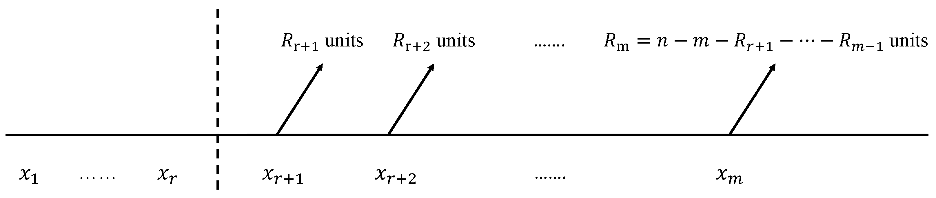
As for general progressive Type-II censoring (referenced in [15], Chapter 1.5, page 9), it is a more general and flexible form of the progressive Type-II censoring, which allows the experimenters to lose the first r observations (which means they only know the number but without exact time of the failures) before they start to perform the progressive censoring. Consequently, the censoring scheme evolved into $(R_{r+1},R_{r+2},\cdots ,R_m)$, signifying that censoring initiates upon the $(r+1)$th failure. The entire procedure is explained in Figure 3. Many scholars have discussed this type of CS. For example, ref. [18] estimated the exponential parameters by utilizing classical and Bayesian perspectives. Ref. [19] investigated a competing risks model utilizing the general censored samples, while ref. [20] introduced a novel solution to assess if the general progressively Type-II censored samples follow the exponential distribution.

In this study, given the well flexibility and extensibility of both GIED and the general progressive Type-II censoring, and on the purpose of further reduce the cost and minimizing the time of the life tests, we consider a combination of ALT and censoring, focusing on the statistical inferences on the generalized inverted exponential distribution using general progressively censored data under a constant stress partially accelerated life test. It is worth noting that although this framework is useful and important, it has not been well studied. Ref. [21] studied the statistical inferences of the GIED based on joint progressively type-II censoring, which did not involve the CSPALT. In the next section, we will discuss the specific model and relevant assumptions, and then we derive the point and interval estimation of the parameters of GIED as well as the acceleration factor from both classical and Bayesian view. For comparison, we conduct Monte-Carlo simulations to evaluate the performance of different methods. In the end, a real lifetime dataset is utilized to justify the applicability of the proposed model and methods.

2. Model and Assumptions

2.1. Model

(1)

Testing process for n units involves dividing them into two groups: the first group comprises $n_1$ randomly selected items from the normal condition test items, while the second group includes the remaining $n_2$ items ($n_1+n_2=n$), which are set under the accelerated condition.

(2)

Each group is tested using general progressive Type-II censoring with fixed sizes, denoted by $(n_j,m_j)$, where for group $j\in \{1,2\}$, $m_j$ represents the known count of the failures for both normal and stress circumstances. Let the vector $(R_{j,r_j+1},R_{j,r_j+2},\cdots ,R_{j,m_j})$ denote the censoring scheme, and the resulting observations for each group are expressed as $(X_{j,r_j+1},X_{j,r_j+2},\cdots ,X_{j,m_j})$.

2.2. Assumptions

(1)

The lifetime of each individual product set in normal condition follows the generalized inverted exponential distribution independently and identically, with the functions provided in (1).

(2)

The HRF of any product set in accelerated condition is given as $H_2\left(x\right)=\beta H_1\left(x\right)$, in which $\beta >1$ represents the acceleration factor.

Then, based on the functions described in (1) and the proposed assumptions, PDF, CDF, SF and HRF of the lifetime of each unit under the accelerated condition can be expressed as shown below:

$$\begin{array}{cc}\hfill f_2\left(x\right)=& \beta \alpha \lambda x^{-2}{e}^{-\frac{\lambda }{x}}{\left(1-e^{-\frac{\lambda }{x}}\right)}^{\beta \alpha -1},\hfill \\ \hfill F_2\left(x\right)=& 1-{\left(1-e^{-\frac{\lambda }{x}}\right)}^{\beta \alpha },\hfill \\ \hfill S_2\left(x\right)=& {\left(1-e^{-\frac{\lambda }{x}}\right)}^{\beta \alpha },\hfill \\ \hfill H_2\left(x\right)=& \beta \alpha \lambda x^{-2}{e}^{-\frac{\lambda }{x}}{\left(1-e^{-\frac{\lambda }{x}}\right)}^{-1},\hfill \end{array}$$

(2)

where $x>0;\alpha ,\lambda >0;\beta >1$. Therefore, if the lifetime of the $n_j,j=1,2$ units follows the GIED with $f_j\left(x\right)$ as PDF and $F_j\left(x\right)$ as CDF, then according to [15], Page 10, the joint density function for $(X_{j,r_j+1},X_{j,r_j+2},\cdots ,X_{j,m_j})$ with CS $(R_{j,r_j+1},R_{j,r_j+2},\cdots ,R_{j,m_j})$ can be given by:

$$L=\prod _{j=1}^2{A}_j{\left[F_j\left(x_{j,r_j+1}\right)\right]}^{r_j}\prod _{i=r_{j+1}}^{m_j}{f}_j\left(x_{ji}\right){\left[1-F_j\left(x_{ji}\right)\right]}^{R_{ji}},$$

(3)

where $x_{ji}$, $j=1,2$, $i=r_j+1,r_j+2,\cdots ,m_j$, is the observed $m_j-r_j$ failure times, and

$$A_j=\frac{n_j!}{r_j!\left(n_j-r_j-1\right)!}\left(n_j-R_{j,r_j+1}-r_j-1\right)\cdots \left(n_j-R_{j,r_j+1}\cdots -R_{j,m_j-1}-m_j+1\right).$$

3. Classical Inferences

3.1. Maximum Likelihood Method

Consider $j\in \{1,2\}$, let $X_{j,r_j+1}<X_{j,r_j+2}<\cdots <X_{j,m_j}$ refer to the general progressively Type-II censored samples from GIED concerning CS $(R_{j,r_j+1},R_{j,r_j+2},\cdots ,R_{j,m_j})$, where the subscript j represents the two different testing conditions. The related PDF and CDF are given in (1) and (2). Therefore, the logarithmic form of the likelihood function is derived as shown below:

$$\begin{array}{cc}\hfill l(\alpha ,\lambda ,\beta )=& ln{A}_1+ln{A}_2+\left(m_1-r_1\right)ln\alpha \lambda +\left(m_2-r_2\right)ln\beta \alpha \lambda \hfill \\ \hfill & +r_{1}ln\left[1-{\left(1-e^{-\lambda /x_{1,r_1+1}}\right)}^{\alpha }\right]+r_{2}ln\left[1-{\left(1-e^{-\lambda /x_{2,r_2+1}}\right)}^{\beta \alpha }\right]\hfill \\ \hfill & -2\left(\sum _{i=r_1+1}^{m_1}ln{x}_{1i}+\sum _{i=r_2+1}^{m_2}ln{x}_{2i}\right)-\lambda \left(\sum _{i=r_1+1}^{m_1}\frac{1}{x_{1i}}+\sum _{i=r_2+1}^{m_2}\frac{1}{x_{2i}}\right)\hfill \\ \hfill & +(\alpha -1)\sum _{i=r_1+1}^{m_1}ln\left(1-e^{-\lambda /x_{1i}}\right)+(\beta \alpha -1)\sum _{i=r_2+1}^{m_2}ln\left(1-e^{-\lambda /x_{2i}}\right)\hfill \\ \hfill & +\alpha \sum _{i=r_1+1}^{m_1}{R}_{1i}ln\left(1-e^{-\lambda /x_{1i}}\right)+\beta \alpha \sum _{i=r_2+1}^{m_2}{R}_{2i}ln\left(1-e^{-\lambda /x_{2i}}\right),\hfill \end{array}$$

(4)

then upon computing the first partial derivatives of $l(\alpha ,\lambda ,\beta )$ concerning the three parameters and making them equal to 0, one arrives at the set of equations below:  

$$\begin{array}{cc}\hfill \frac{\partial l}{\partial \alpha }=& (m_1+m_2-r_1-r_2)\frac{1}{\alpha }\hfill \\ \hfill & -\frac{r_1{\left(1-e^{-\lambda /x_{1,r_1+1}}\right)}^{\alpha }ln\left(1-e^{-\lambda /x_{1,r_1+1}}\right)}{1-{\left(1-e^{-\lambda /x_{1,r_1+1}}\right)}^{\alpha }}\hfill \\ \hfill & -\frac{\beta r_2{\left(1-e^{-\lambda /x_{2,r_2+1}}\right)}^{\beta \alpha }ln\left(1-e^{-\lambda /x_{2,r_2+1}}\right)}{1-{\left(1-e^{-\lambda /x_{2,r_2+1}}\right)}^{\beta \alpha }}\hfill \\ \hfill & +\sum _{i=r_1+1}^{m_1}ln\left(1-e^{-\lambda /x_{1i}}\right)+\beta \sum _{i=r_2+1}^{m_2}ln\left(1-e^{-\lambda /x_{2i}}\right)\hfill \\ \hfill & +\sum _{i=r_1+1}^{m_1}{R}_{1i}ln\left(1-e^{-\lambda /x_{1i}}\right)+\beta \sum _{i=r_2+1}^{m_2}{R}_{2i}ln\left(1-e^{-\lambda /x_{2i}}\right)=0,\hfill \end{array}$$

(5)

$$\begin{array}{cc}\hfill \frac{\partial l}{\partial \lambda }=& \left(m_1+m_2-r_1-r_2\right)\frac{1}{\lambda }-\sum _{i=r_1+1}^{m_1}\frac{1}{x_{1i}}-\sum _{i=r_2+1}^{m_2}\frac{1}{x_{2i}}\hfill \\ \hfill & -\frac{\alpha r_1{\left(1-e^{-\lambda /x_{1,r_1+1}}\right)}^{\alpha -1}{e}^{-\lambda /x_{1,r_1+1}}}{\left[1-{\left(1-e^{-\lambda /x_{1,r_1+1}}\right)}^{\alpha }\right]x_{1,r_1+1}}-\frac{\beta \alpha r_2{\left(1-e^{-\lambda /x_{2,r_2+1}}\right)}^{\beta \alpha -1}{e}^{-\lambda /x_{2,r_2+1}}}{\left[1-{\left(1-e^{-\lambda /x_{2,r_2+1}}\right)}^{\beta \alpha }\right]x_{2,r_2+1}}\hfill \\ \hfill & +(\alpha -1)\sum _{i=r_1+1}^{m_1}\frac{e^{-\lambda /x_{1i}}}{\left(1-e^{-\lambda /x_{1i}}\right)x_{1i}}+(\beta \alpha -1)\sum _{i=r_2+1}^{m_2}\frac{e^{-\lambda /x_{2i}}}{\left(1-e^{-\lambda /x_{2i}}\right)x_{2i}}\hfill \\ \hfill & +\alpha \sum _{i=r_1+1}^{m_1}{R}_{1i}\frac{e^{-\lambda /x_{1i}}}{\left(1-e^{-\lambda /x_{1i}}\right)x_{1i}}+\beta \alpha \sum _{i=r_2+1}^{m_2}{R}_{2i}\frac{e^{-\lambda /x_{2i}}}{\left(1-e^{-\lambda /x_{2i}}\right)x_{2i}}=0\hfill \end{array}$$

(6)

and

$$\begin{array}{cc}\hfill \frac{\partial l}{\partial \beta }=& (m_2-r_2)\frac{1}{\beta }-\frac{\alpha r_2{\left(1-e^{-\lambda /x_{2,r_2+1}}\right)}^{\beta \alpha }ln\left(1-e^{-\lambda /x_{2,r_2+1}}\right)}{1-{\left(1-e^{-\lambda /x_{2,r_2+1}}\right)}^{\beta \alpha }}\hfill \\ \hfill & +\alpha \sum _{i=r_2+1}^{m_2}ln\left(1-e^{-\lambda /x_{2i}}\right)+\alpha \sum _{i=r_2+1}^{m_2}{R}_{2i}ln\left(1-e^{-\lambda /x_{2i}}\right)=0.\hfill \end{array}$$

(7)

The MLEs of $\alpha$, $\lambda$ and $\beta$ symbolized by $\widehat{\alpha }$, $\widehat{\lambda }$ and $\widehat{\beta }$, are then derived from Equations (5)–(7). Due to the challenge of obtaining the precise analytical solution, we utilize the function ‘optim’ in R to derive the MLEs of the three parameters. In addition, one can obtain the MLE of the mean of the GIED straightforwardly due to the invariance property of MLE. According to [3], the mean $\mu$ of GIED is

$$\mu ={\int }_0^{\infty }{S}_1\left(x\right)\mathrm{d}x={\int }_0^{\infty }{\left[1-exp\left(-\frac{\lambda }{x}\right)\right]}^{\alpha }\mathrm{d}x,$$

so the MLE of the mean $\mu$ is

$$\widehat{\mu }={\int }_0^{\infty }{\left[1-exp\left(-\frac{\widehat{\lambda }}{x}\right)\right]}^{\widehat{\alpha }}\mathrm{d}x.$$

3.2. Approximate Confidence Intervals

Because there are no closed-form solutions available for the MLEs, the precise bounds of the confidence intervals (CIs) for these parameters are impossible to be derived. Hence, we resort to establishing approximate confidence intervals (ACIs) for the three parameters using the Fisher information matrix.

Denote $\mathit{\theta }={(\alpha ,\lambda ,\beta )}^{\top }$, then the asymptotic covariance matrix denoted as $I{\left(\mathit{\theta }\right)}^{-1}$ is utilized to obtain the approximate CIs. $I{\left(\mathit{\theta }\right)}^{-1}$ is given by:

$$\begin{array}{cc}\hfill I{\left(\mathit{\theta }\right)}^{-1}& =-{\left(\begin{array}{ccc}\frac{{\partial }^{2}l}{\partial {\alpha }^2}\hfill & \frac{{\partial }^{2}l}{\partial \alpha \partial \lambda }\hfill & \frac{{\partial }^{2}l}{\partial \alpha \partial \beta }\hfill \\ \frac{{\partial }^{2}l}{\partial \lambda \partial \alpha }\hfill & \frac{{\partial }^{2}l}{\partial {\lambda }^2}\hfill & \frac{{\partial }^{2}l}{\partial \lambda \partial \beta }\hfill \\ \frac{{\partial }^{2}l}{\partial \beta \partial \alpha }\hfill & \frac{{\partial }^{2}l}{\partial \beta \partial \lambda }\hfill & \frac{{\partial }^{2}l}{\partial {\beta }^2}\hfill \end{array}\right)}^{-1}\hfill \\ \hfill & \approx \left(\begin{array}{ccc}Var\left(\widehat{\alpha }\right)\hfill & Cov(\widehat{\alpha },\widehat{\lambda })\hfill & Cov(\widehat{\alpha },\widehat{\beta })\hfill \\ Cov(\widehat{\lambda },\widehat{\alpha })\hfill & Var\left(\widehat{\lambda }\right)\hfill & Cov(\widehat{\lambda },\widehat{\beta })\hfill \\ Cov(\widehat{\beta },\widehat{\alpha })\hfill & Cov(\widehat{\beta },\widehat{\lambda })\hfill & Var\left(\widehat{\beta }\right)\hfill \end{array}\right)\hfill \end{array}$$

(8)

The detailed expressions of the second derivatives of the log-likelihood function are given in Appendix A. Given that $\sqrt{n}(\widehat{\mathit{\theta }}-\mathit{\theta })$ conforms to a multivariate normal distribution (the asymptotic distribution of MLEs) featuring the covariance matrix described by (8) and an expectation vector of zero. Subsequently, the $100(1-\tau )\%$ ACIs are eventually expressed as shown below:

$$\begin{array}{c}\hfill \left[\widehat{\alpha }\pm z_{\tau /2}\sqrt{Var\left(\widehat{\alpha }\right)}\right],\left[\widehat{\lambda }\pm z_{\tau /2}\sqrt{Var\left(\widehat{\lambda }\right)}\right],\left[\widehat{\beta }\pm z_{\tau /2}\sqrt{Var\left(\widehat{\beta }\right)}\right].\end{array}$$

(9)

4. Bayesian Method

4.1. Prior Information

For this part, we assume independent gamma distributions as the prior distributions for the three random variables ($\alpha$, $\lambda$, and $\beta -1$). That is, $\alpha \sim \mathrm{Gamma}(a_1,b_1)$, $\lambda \sim \mathrm{Gamma}(a_2,b_2)$ and $\beta -1\sim \mathrm{Gamma}(a_3,b_3)$. After that, the joint prior density $\pi (\alpha ,\lambda ,\beta )$ is formulated as shown below:

$$\begin{array}{c}\hfill \pi (\alpha ,\lambda ,\beta )\propto {\alpha }^{a_1-1}{\lambda }^{a_2-1}{(\beta -1)}^{a_3-1}{e}^{-(b_1\alpha +b_2\lambda +b_3(\beta -1))},\end{array}$$

(10)

where $a_1,b_1,a_2,b_2$ and $a_3,b_3$ are hyper-parameters. They are non-negative and pre-determined. Independent gamma distributions has been chosen as the priors because of the adaptable nature of the gamma distribution.

Then the joint posterior density function is derived with regard for the formulated likelihood and prior density functions:

$$\begin{array}{cc}\hfill \pi (\alpha ,\lambda ,\beta \mid \mathit{x})=& C^{-1}{\alpha }^{m_1+m_2-r_1-r_2+a_1-1}{\lambda }^{m_1+m_2-r_1-r_2+a_2-1}{\beta }^{m_2-r_2}{(\beta -1)}^{a_3-1}{e}^{-\left(b_1\alpha +b_2\lambda +b_3(\beta -1)\right)}\hfill \\ \hfill & \times {\left[1-{\left(1-e^{-\lambda /x_{1,r_1+1}}\right)}^{\alpha }\right]}^{r_1}{\left[1-{\left(1-e^{-\lambda /x_{2,r_2+1}}\right)}^{\beta \alpha }\right]}^{r_2}\hfill \\ \hfill & \times \prod _{i=r_1+1}^{m_1}\frac{1}{x_{1i}^2}{e}^{-\lambda /x_{1i}}{\left(1-e^{-\lambda /x_{1i}}\right)}^{\alpha R_{1i}+\alpha -1}\hfill \\ \hfill & \times \prod _{i=r_2+1}^{m_2}\frac{1}{x_{2i}^2}{e}^{-\lambda /x_{2i}}{\left(1-e^{-\lambda /x_{2i}}\right)}^{\beta \alpha R_{2i}+\beta \alpha -1},\hfill \end{array}$$

(11)

where $\mathit{x}$ denotes the data, and

$$\begin{array}{cc}\hfill C={\int }_0^{\infty }{\int }_0^{\infty }{\int }_0^{\infty }& {\alpha }^{m_1+m_2-r_1-r_2+a_1-1}{\lambda }^{m_1+m_2-r_1-r_2+a_2-1}{\beta }^{m_2-r_2}{(\beta -1)}^{a_3-1}{e}^{-\left(b_1\alpha +b_2\lambda +b_3(\beta -1)\right)}\hfill \\ \hfill & \times {\left[1-{\left(1-e^{-\lambda /x_{1,r_1+1}}\right)}^{\alpha }\right]}^{r_1}{\left[1-{\left(1-e^{-\lambda /x_{2,r_2+1}}\right)}^{\beta \alpha }\right]}^{r_2}\hfill \\ \hfill & \times \prod _{i=r_1+1}^{m_1}\frac{1}{x_{1i}^2}{e}^{-\lambda /x_{1i}}{\left(1-e^{-\lambda /x_{1i}}\right)}^{\alpha R_{1i}+\alpha -1}\hfill \\ \hfill & \times \prod _{i=r_2+1}^{m_2}\frac{1}{x_{2i}^2}{e}^{-\lambda /x_{2i}}{\left(1-e^{-\lambda /x_{2i}}\right)}^{\beta \alpha R_{2i}+\beta \alpha -1}d\alpha d\lambda d\beta .\hfill \end{array}$$

(12)

Thereafter, the formula for obtaining the Bayesian estimate of an arbitrary function $h(\alpha ,\lambda ,\beta )$ using the squared error loss function (SELF) may be provided by:

$$\begin{array}{cc}\hfill \tilde{h}(\alpha ,\lambda ,\beta )=& {\mathrm{E}}_{\alpha ,\lambda ,\beta \mid \mathit{x}}\left[h(\alpha ,\lambda ,\beta )\right]\hfill \\ \hfill =& {\int }_0^{\infty }{\int }_0^{\infty }{\int }_0^{\infty }h(\alpha ,\lambda ,\beta )\pi (\alpha ,\lambda ,\beta \mid \mathit{x})d\alpha d\lambda d\beta ,\hfill \end{array}$$

(13)

obviously it is impossible to compute (13), it is for this reason that the importance sampling approach is then utilized to establish the Bayesian point estimates. Additionally, we employ the same methodology to create the Bayesian credible intervals (BCIs) and the highest posterior density credible intervals (HPDCIs).

4.2. Posterior Analysis

To apply the importance sampling method, posterior density function is first expressed as shown below:

$$\begin{array}{c}\hfill \pi (\alpha ,\lambda ,\beta \mid \mathit{x})\propto g_{\lambda }(u_1,v_1)\times g_{\alpha \mid \lambda }(u_2,v_2)\times g_{(\beta -1)\mid \alpha ,\lambda }(u_3,v_3)\times q(\alpha ,\lambda ,\beta ),\end{array}$$

(14)

where $g_{\lambda }(u_1,v_1)$, $g_{\alpha \mid \lambda }(u_2,v_2)$, and $g_{(\beta -1)\mid \alpha ,\lambda }(u_3,v_3)$ represent gamma density functions with parameters given by:

$$u_1=m_1+m_2-r_1-r_2+a_2$$

$$v_1=b_2+\sum _{i=r_1+1}^{m_1}\frac{1}{x_{1i}}+\sum _{i=r_2+1}^{m_2}\frac{1}{x_{2i}},$$

$$u_2=m_1+m_2-r_1-r_2+a_1$$

$$v_2=b_1-\sum _{i=r_1+1}^{m_1}(1+R_{1i})ln(1-e^{-\lambda /x_{1i}})-\sum _{i=r_2+1}^{m_2}(1+R_{2i})ln(1-e^{-\lambda /x_{2i}})$$

and

$$u_3=\frac{1}{2}{m}_2+\frac{1}{2}{r}_2+a_3$$

$$v_3=b_3-\sum _{i=r_2+1}^{m_2}\alpha (1+R_{2i})ln(1-e^{-\lambda /x_{2i}}),$$

also, $q(\alpha ,\lambda ,\beta )$ is given by:

$$\begin{array}{c}\hfill q(\alpha ,\lambda ,\beta )=\frac{q^{\prime }(\alpha ,\lambda ,\beta )}{v_2^{u_2}{v}_3^{u_3}},\end{array}$$

(15)

where

$$\begin{array}{cc}\hfill q^{\prime }(\alpha ,\lambda ,\beta )=& {\beta }^{m_2-r_2}{(\beta -1)}^{\frac{r_2}{2}-\frac{m_2}{2}}{\left[1-{(1-e^{-\lambda /x_{1,r_1+1}})}^{\alpha }\right]}^{r_1}{\left[1-{(1-e^{-\lambda /x_{2,r_2+1}})}^{\beta \alpha }\right]}^{r_2}\hfill \\ \hfill & \times exp\left\{-\sum _{i=r_1+1}^{m_1}ln\left[x_{1i}^2(1-e^{-\lambda /x_{1i}})\right]-\sum _{i=r_2+1}^{m_2}ln\left[x_{2i}^2(1-e^{-\lambda /x_{2i}})\right]\right\}.\hfill \end{array}$$

(16)

After that, it is possible to utilize the importance sampling to derive the Bayesian estimation and the relative BCIs. The specific steps of the method are shown below:

Step 1:

Generate a random variable ${\lambda }_1$ from $\mathrm{Gamma}(u_1,v_1)$.

Step 2:

Generate a random variable ${\alpha }_1$ from $\mathrm{Gamma}(u_2,v_2)$.

Step 3:

Generate a random variable ${\beta }_1^{\prime }$ from $\mathrm{Gamma}(u_3,v_3)$, and set ${\beta }_1={\beta }_1^{\prime }+1$.

Step 4:

Perform Steps 1–3 a total of D times to generate (${\lambda }_1,\cdots ,{\lambda }_D$), (${\alpha }_1,\cdots ,{\alpha }_D$) and (${\beta }_1,\cdots ,{\beta }_D$).

Step 5:

Derive the BEs under SELF as

$$\tilde{\alpha }=\frac{{\sum }_{i=1}^D{\alpha }_{i}q({\alpha }_i,{\lambda }_i,{\beta }_i)}{{\sum }_{i=1}^{D}q({\alpha }_i,{\lambda }_i,{\beta }_i)},\tilde{\lambda }=\frac{{\sum }_{i=1}^D{\lambda }_{i}q({\alpha }_i,{\lambda }_i,{\beta }_i)}{{\sum }_{i=1}^{D}q({\alpha }_i,{\lambda }_i,{\beta }_i)}$$

and

$$\tilde{\beta }=\frac{{\sum }_{i=1}^D{\beta }_{i}q({\alpha }_i,{\lambda }_i,{\beta }_i)}{{\sum }_{i=1}^{D}q({\alpha }_i,{\lambda }_i,{\beta }_i)}.$$

The $100(1-\tau )\%$ HPDCIs are constructed through the same method of [22]. For the sake of concision, only the BCI and corresponding HPDCI of the parameter $\beta$ are discussed here, the intervals for the other two parameters can be obtained using the same procedure.

Assume that for $0<p<1$, ${\beta }_p$ satisfies $\mathit{P}[\beta \le {\beta }_p\mid x]=p$. Then a more intricate approach involves deriving a consistent estimator of ${\beta }_p$ using the SELF based on the produced sample $({\alpha }_1,{\lambda }_1,{\beta }_1),\cdots ,({\alpha }_D,{\lambda }_D,{\beta }_D)$. Let

$$u_i=\frac{q({\alpha }_i,{\lambda }_i,{\beta }_i)}{{\sum }_{i=1}^{D}q({\alpha }_i,{\lambda }_i,{\beta }_i)},i=1,\cdots D,$$

reorganize $\{({\beta }_1,u_1),\cdots ,({\beta }_D,u_D)\}$ to be $\{({\beta }_{\left(1\right)},u_{\left(1\right)}),\cdots ,({\beta }_{\left(D\right)},u_{\left(D\right)})\}$, in which ${\beta }_{\left(1\right)}<\cdots <{\beta }_{\left(D\right)}$. It is worth noting that the $u_{\left(i\right)}$’s are not arranged in any specific order, they are simply correlated with the ${\beta }_{\left(i\right)}$’s. Then a consistent Bayesian estimator of ${\beta }_p$ is ${\tilde{\beta }}_p^{*}={\beta }_{\left(M_p\right)}$, with the integer $M_p$ satisfying the condition below:

$$\sum _{i=1}^{M_p}{u}_{\left(i\right)}\le p\le \sum _{i=1}^{M_p+1}{u}_{\left(i\right)}.$$

Utilizing the outlined procedure, a $100(1-\tau )\%$ BCI of $\beta$ is computed to be $\left({\tilde{\beta }}_{\nu }^{*},{\tilde{\beta }}_{\nu +1-\tau }^{*}\right)$, for $\nu =u_{\left(1\right)},u_{\left(1\right)}+u_{\left(2\right)},\cdots ,{\sum }_{i=1}^{M_{\tau }}{u}_{\left(i\right)}$. Accordingly, an HPDCI of $\beta$ with a significance level $\tau$ can be expressed as $\left({\tilde{\beta }}_{{\nu }^{*}}^{*},{\tilde{\beta }}_{{\nu }^{*}+1-\tau }^{*}\right)$, and ${\nu }^{*}$ meets the inequality constraint:

$${\tilde{\beta }}_{{\nu }^{*}+1-\tau }^{*}-{\tilde{\beta }}_{{\nu }^{*}}^{*}\le {\tilde{\beta }}_{\nu +1-\tau }^{*}-{\tilde{\beta }}_{\nu }^{*},\mathrm{for}\mathrm{all}\nu .$$

5. Numerical Simulation

5.1. Monte-Carlo Studies

For this part, we carry out comprehensive Monte-Carlo simulations for the purpose of evaluating the various approaches for estimating the three parameters. For the point estimation, we adopt the mean squared error (MSE) and average bias (AB) since MSE is able to measure the volatility of data, and AB makes up for the disadvantage of MSE that it is sensitive to some extreme values. For the interval estimation, we select average interval length (AL) and the coverage probability (CP), as shorter ALs mean the confidence or credible intervals are more accurate under a fixed significance level, and higher CPs indicates that the confidence or credible intervals are more likely to include the true values of the parameters. The evaluating criteria for assessing the performance of the estimates outlined are shown below:

(1)

Mean squared error (MSE) of the point estimation $\widehat{\varphi }$, which is calculated by $\frac{1}{N}\Sigma {(\widehat{\varphi }-\varphi )}^2$, where $\varphi$ represents each of the three parameters discussed in this model. The number of replications is denoted by N;

(2)

Average bias (AB) of the point estimation $\widehat{\varphi }$, which is calculated by $\frac{1}{N}\Sigma \mid \widehat{\varphi }-\varphi \mid$;

(3)

Average length (AL) of the confidence or credible intervals (CIs) of $\varphi$ with a significance level $\tau$;

(4)

Coverage probability (CP) of the $100(1-\tau )\%$ CIs of $\varphi$, which reflects the proportion of instances where the actual parameter values lie in the calculated intervals.

To be concise, we take $n_1=n_2=n$, $m_1=m_2=m$ and $r_1=r_2=r$, running simulations under both normal and accelerated conditions with the following CSs:

CS [1]:

$n=25$, $m=20$, $r=5$, $R_{j1}=\cdots =R_{j5}=1$, $R_{j6}=\cdots =R_{j,15}=0$;

CS [2]:

$n=30$, $m=20$, $r=5$, $R_{j1}=\cdots =R_{j5}=2$, $R_{j6}=\cdots =R_{j,15}=0$;

CS [3]:

$n=25$, $m=20$, $r=5$, $R_{j,11}=\cdots =R_{j,15}=1$, $R_{j1}=\cdots =R_{j,10}=0$;

CS [4]:

$n=35$, $m=30$, $r=5$, $R_{j1}=\cdots =R_{j5}=1$, $R_{j6}=\cdots =R_{j,25}=0$;

CS [5]:

$n=40$, $m=30$, $r=5$, $R_{j1}=\cdots =R_{j5}=2$, $R_{j6}=\cdots =R_{j,25}=0$;

CS [6]:

$n=35$, $m=30$, $r=5$, $R_{j,21}=\cdots =R_{j,25}=1$, $R_{j1}=\cdots =R_{j,20}=0$;

CS [7]:

$n=55$, $m=50$, $r=5$, $R_{j1}=\cdots =R_{j5}=1$, $R_{j6}=\cdots =R_{j,45}=0$;

CS [8]:

$n=60$, $m=50$, $r=5$, $R_{j1}=\cdots =R_{j5}=2$, $R_{j6}=\cdots =R_{j,45}=0$;

CS [9]:

$n=55$, $m=50$, $r=5$, $R_{j,41}=\cdots =R_{j,45}=1$, $R_{j1}=\cdots =R_{j,40}=0$.

Based on the above evaluating criteria and the censoring schemes, two sets of parameter values are taken into consideration for our Monte-Carlo studies, which are ${\mathit{\theta }}_{\mathbf{1}}=(\alpha ,\lambda ,\beta )=(0.8,0.5,1.5)$ and ${\mathit{\theta }}_{\mathbf{2}}=(\alpha ,\lambda ,\beta )=(1,0.8,2)$, respectively. In terms of the Bayesian estimate, the corresponding hyper-parameters are chosen as $(a_1,b_1,a_2,b_2,a_3,b_3)=(1.6,2,1,2,1,2)$ and $(a_1,b_1,a_2,b_2,a_3,b_3)=(4,4,3.2,4,4,4)$, which indicate the expectations of the three Gamma distributions as the prior, respectively. It makes sense that when choosing the more accurate priors, we may obtain better estimates. It is to be noted that the hyper-parameters should not be too large, since it may mask the effects of the three newly-constructed Gamma distributions, which led us to setting the hyper-parameters as above. The method in [15] is performed regarding the production of the general progressively censored sample under the pre-determined CS $(R_{r+1},R_{r+2},\cdots ,R_m)$, and the specific algorithms are shown below:

Since this sort of censored sample can be obtained based on Algorithm 1, it is possible to generate sample under general progressive censoring by Algorithm 2.

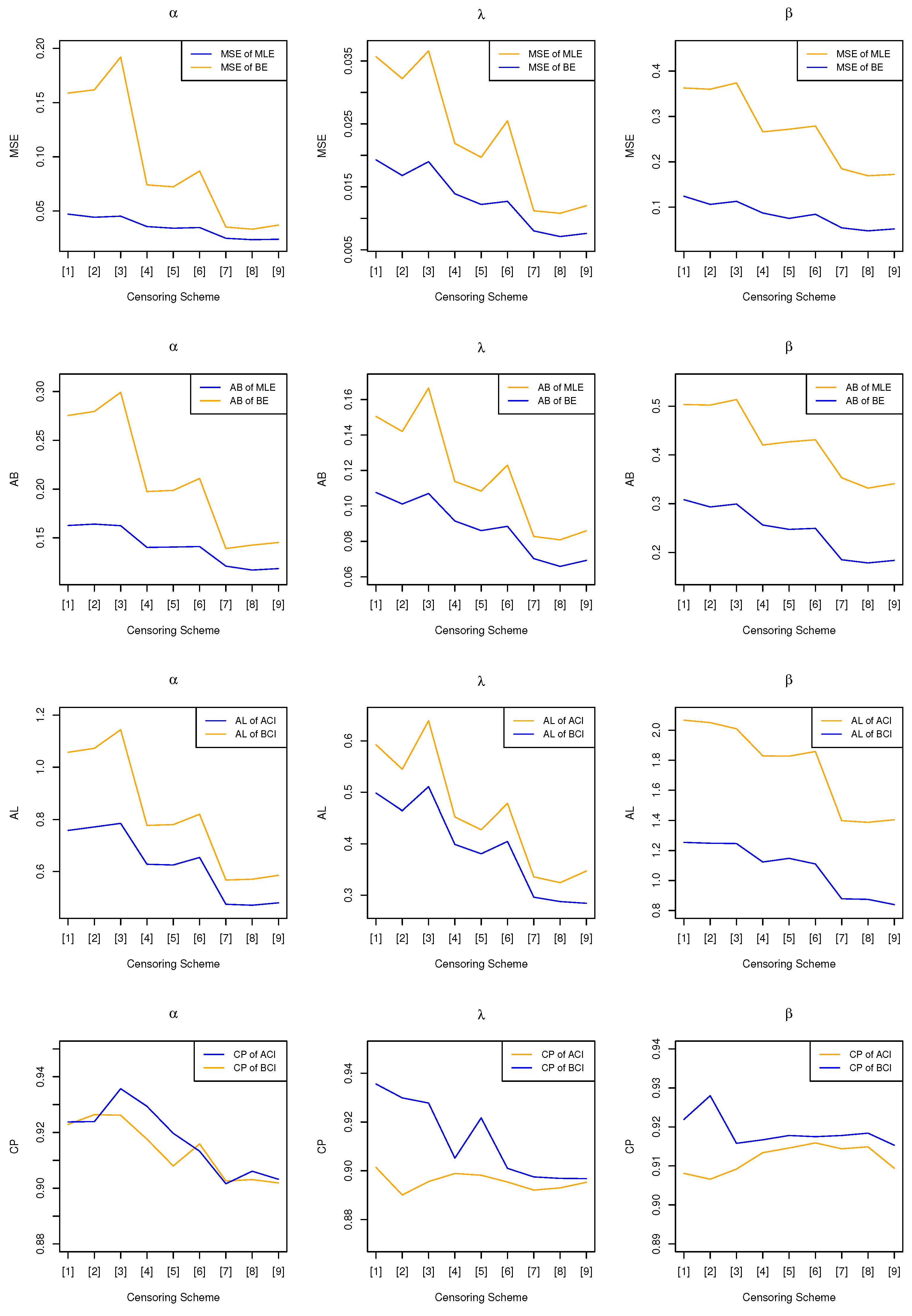
Different estimates adopting both classical and Bayesian viewpoint for the three parameters and the corresponding evaluating criteria (EC) are calculated with sample generated from both normal and accelerated conditions utilizing general progressively Type-II censoring under multiple CSs. Specifically, the MSEs and ABs of the point estimation are shown in

Table 1. MSEs and ABs of the estimates for the parameters ${\mathit{\theta }}_{\mathbf{1}}$ and ${\mathit{\theta }}_{\mathbf{2}}$.

		${\mathit{\theta }}_{\mathbf{1}}$						${\mathit{\theta }}_{\mathbf{2}}$
		MLE			BE			MLE			BE
CS	EC	α	λ	β	α	λ	β	α	λ	β	α	λ	β
[1]	MSE	0.0991	0.0223	0.2516	0.0440	0.0196	0.1098	0.1588	0.0357	0.3628	0.0471	0.0193	0.1242
	AB	0.2186	0.1111	0.3732	0.1547	0.1076	0.2515	0.2755	0.1505	0.5035	0.1627	0.1076	0.3083
[2]	MSE	0.0940	0.0173	0.2484	0.0442	0.0130	0.1025	0.1618	0.0322	0.3601	0.0442	0.0168	0.1062
	AB	0.2126	0.0990	0.3693	0.1541	0.0867	0.2413	0.2796	0.1420	0.5023	0.1641	0.1011	0.2934
[3]	MSE	0.1163	0.0265	0.2588	0.0494	0.0177	0.1027	0.1920	0.0366	0.3739	0.0452	0.0190	0.1129
	AB	0.2317	0.1201	0.3760	0.1615	0.1000	0.2511	0.2992	0.1665	0.5136	0.1625	0.1070	0.2994
[4]	MSE	0.0451	0.0114	0.1872	0.0276	0.0134	0.0639	0.0741	0.0219	0.2662	0.0356	0.0139	0.0872
	AB	0.1558	0.0817	0.3319	0.1254	0.0900	0.1903	0.1975	0.1138	0.4205	0.1402	0.0915	0.2564
[5]	MSE	0.0464	0.0099	0.1861	0.0259	0.0096	0.0624	0.0723	0.0197	0.2719	0.0341	0.0122	0.0753
	AB	0.1560	0.0760	0.3321	0.1213	0.0756	0.1882	0.1987	0.1084	0.4269	0.1406	0.0861	0.2474
[6]	MSE	0.0513	0.0130	0.2027	0.0272	0.0106	0.0598	0.0868	0.0255	0.2790	0.0347	0.0127	0.0844
	AB	0.1621	0.0861	0.3408	0.1235	0.0789	0.1892	0.2109	0.1230	0.4312	0.1411	0.0885	0.2495
[7]	MSE	0.0217	0.0069	0.1077	0.0168	0.0073	0.0464	0.0352	0.0112	0.1847	0.0248	0.0080	0.0545
	AB	0.1128	0.0715	0.2544	0.0999	0.0722	0.1586	0.1391	0.0828	0.3533	0.1210	0.0703	0.1851
[8]	MSE	0.0210	0.0063	0.1047	0.0160	0.0057	0.0454	0.0332	0.0108	0.1693	0.0235	0.0071	0.0479
	AB	0.1099	0.0672	0.2502	0.0968	0.0648	0.1564	0.1426	0.0809	0.3320	0.1170	0.0659	0.1786
[9]	MSE	0.0232	0.0067	0.1074	0.0158	0.0063	0.0427	0.0370	0.0120	0.1723	0.0239	0.0076	0.0521
	AB	0.1152	0.0685	0.2533	0.0951	0.0661	0.1576	0.1453	0.0860	0.3411	0.1185	0.0693	0.1838

, and the ALs and CPs of the interval estimation are given in

Table 2. ALs and CPs of the intervals for the parameters ${\mathit{\theta }}_{\mathbf{1}}$ and ${\mathit{\theta }}_{\mathbf{2}}$ with τ = 0.10.

		${\mathit{\theta }}_{\mathbf{1}}$						${\mathit{\theta }}_{\mathbf{2}}$
		ACI			BCI			ACI			BCI
CS	EC	α	λ	β	α	λ	β	α	λ	β	α	λ	β
[1]	AL	0.8303	0.4191	1.7075	0.6306	0.3429	0.8896	1.0574	0.5925	2.0670	0.7581	0.4984	1.2544
	CP	0.8331	0.8853	0.8797	0.8603	0.8915	0.9165	0.9229	0.9014	0.9081	0.9238	0.9356	0.9219
[2]	AL	0.8329	0.3823	1.7123	0.6513	0.3337	0.8826	1.0727	0.5448	2.0507	0.7715	0.4642	1.2488
	CP	0.8375	0.8974	0.8834	0.9157	0.9018	0.9209	0.9264	0.8901	0.9066	0.9239	0.9299	0.9280
[3]	AL	0.8909	0.4499	1.7356	0.6838	0.3946	1.0461	1.1444	0.6393	2.0095	0.7853	0.5108	1.2467
	CP	0.8368	0.8868	0.8898	0.9186	0.8980	0.9217	0.9262	0.8956	0.9092	0.9357	0.9278	0.9158
[4]	AL	0.6146	0.3170	1.3537	0.5082	0.2823	0.8864	0.7775	0.4523	1.8291	0.6281	0.3988	1.1236
	CP	0.8243	0.8812	0.8801	0.8959	0.8873	0.9218	0.9176	0.8989	0.9134	0.9294	0.9052	0.9167
[5]	AL	0.6187	0.2982	1.3559	0.5061	0.2713	0.8700	0.7805	0.4275	1.8271	0.6252	0.3806	1.1480
	CP	0.8453	0.8893	0.8960	0.9259	0.9065	0.9206	0.9080	0.8982	0.9146	0.9197	0.9217	0.9178
[6]	AL	0.6421	0.3320	1.3675	0.5088	0.2901	0.9009	0.8203	0.4783	1.8582	0.6542	0.4046	1.1106
	CP	0.8832	0.8861	0.8806	0.9241	0.9037	0.9194	0.9159	0.8954	0.9159	0.9133	0.9010	0.9175
[7]	AL	0.4480	0.2331	1.0311	0.3739	0.1891	0.6563	0.5675	0.3357	1.3990	0.4742	0.2961	0.8785
	CP	0.8693	0.8984	0.8996	0.9176	0.8971	0.9165	0.9026	0.8921	0.9144	0.9016	0.8975	0.9178
[8]	AL	0.4485	0.2247	1.0273	0.3728	0.1888	0.6505	0.5706	0.3244	1.3883	0.4705	0.2875	0.8748
	CP	0.8905	0.8945	0.9040	0.9265	0.9024	0.9312	0.9031	0.8930	0.9149	0.9061	0.8969	0.9184
[9]	AL	0.4587	0.2389	1.0304	0.3890	0.2037	0.6929	0.5856	0.3471	1.4054	0.4798	0.2842	0.8397
	CP	0.8854	0.8959	0.8942	0.9283	0.9039	0.9244	0.9019	0.8953	0.9094	0.9032	0.8968	0.9153

. In addition, the related plots of the criteria for different parameters are presented in Figure 4 and Figure 5 as well.

Algorithm 1: Generating Progressively Type-II Censored Samples

Step 1: Generate m $\mathrm{Uniform}(0,1)$ random variables $W_1,W_2,\cdots ,W_m$ as observations; Step 2: Let $V_i=W_i^{1/\left(i+{\sum }_{j=m-i+1}^m{R}_j\right)}$, $i=1,2,\cdots ,m$. Step 3: Let $U_i=1-{\prod }_{j=m-i+1}^m{V}_j$, $i=1,2,\cdots ,m$. Consequently, $U_i$’s form the progressively Type-II right censored sample of $\mathrm{Uniform}(0,1)$. Step 4: Let $X_i=F^{-1}\left(U_i\right)$ for each i. $F^{-1}(·)$ denotes the inverse CDF corresponding to the lifetime distribution being studied. Consequently, $X_1,\cdots ,X_m$ constitute the necessary progressively Type-II censored sample of $F(·)$.

Algorithm 2: Generating General Progressively Type-II Censored Samples

Step 1: Generate $U_{r+1}$ from $\mathrm{Beta}(r+1,n-r)$; Step 2: By adopting Algorithm 1, generate $m-r-1$ progressively Type-II censored $\mathrm{Uniform}(0,1)$ samples using CS $(R_{r+2},\cdots ,R_m)$, and they are denoted by $U_{(r+2)},\cdots ,U_{\left(m\right)}$; Step 3: Let $U_i=U_{\left(i\right)}(1-U_{r+1})+U_{r+1}$, $i=r+2,\cdots ,m$, in which $U_{\left(i\right)}$ is as derived according to Step 2; Step 4: Let $X_i=F^{-1}\left(U_i\right)$, for each i. Consequently, $X_{r+1},\cdots ,X_m$ constitute a general progressively Type-II censored sample of $F(·)$.

The findings of the simulation, which are shown in the tables and figures, allow for the formation of several different conclusions:

(1)

In most of the cases, for point estimation and interval estimation, Bayesian method performs better than the classical estimation, with smaller MSEs and ABs, shorter ALs and higher CPs. For example, in terms of the parameter $\alpha$ of ${\mathit{\theta }}_{\mathbf{1}}$ under CS 7-9, one can find from Table 1 that the MSEs for MLE lie around 0.0210 whereas for BE is around 0.0160, with the ALs being about 0.4480 and 0.3739 respectively, which can be seen as a significant advantage of Bayesian method.

(2)

For fixed CSs, both point and interval estimation see a considerable progress when the number of valid samples accumulates. One can see from the two tables that when 10 samples are censored, CS 8 providing $m=50$ valid failure times has much smaller MSEs (0.0210, 0.0160) and ALs (0.4485, 0.3728) than CS 5 and CS 2 (considering $\alpha$ in ${\mathit{\theta }}_{\mathbf{1}}$, for other parameters we can also obtain similar findings), which indicates the consistency of the corresponding estimation.

(3)

However, the performances of both classical and Bayesian method are not satisfying with small samples, providing relatively large MSEs (for instance, around 0.25 for MLE of $\beta$ in ${\mathit{\theta }}_{\mathbf{1}}$) and long intervals (over 1.6 for ACI of $\beta$ in ${\mathit{\theta }}_{\mathbf{1}}$). BEs and BCIs using small samples are slightly better.

It is to be noted that Bayesian method has a distinct advantage over the classical method in the small sample cases, where BEs have much smaller MSEs and ABs and BCIs give much shorter intervals together with relatively higher CPs. In several cases, the CPs can be a bit higher since the CIs are bad with long interval lengths, but with the increasing number of the valid sample, most of the coverage probabilities (CPs) for different CIs are getting closer to the nominal confidence level. For example, the CP of BCI for $\lambda$ in ${\mathit{\theta }}_{\mathbf{2}}$ was higher than 90% under CS 1, but gets closer to 90% (0.8975) due to more valid data under CS 7, with a shorter AL (from 0.4984 to 0.2961). In several situations where the quantity of the units is relatively large, it can be better to have more samples censored at the same time, compared with CSs with less censored samples. In terms of point estimation, for pre-specified valid sample size, the MSEs and ABs of censoring samples at the last five failures are slightly less than those of censoring at the first five failures. In general, both point and interval estimates for parameter $\lambda$ performed the best, featuring considerably small MSEs and ABs, whereas the two estimates of parameter $\beta$ performed the worst, with relatively larger MSEs and longer interval lengths. To be specific, considering the figure of BE for ${\mathit{\theta }}_{\mathbf{1}}$, one can find that the MSE and AB for $\lambda$ under CS 9 are 0.0063 and 0.0661, while for $\beta$ are 0.0427 and 0.1576, which means more deviation on $\beta$ than $\lambda$.

5.2. Real Data Examples

For this part, we examine a real lifetime dataset that records a series of oil breakdown times of a kind of insulating fluid under different stress levels (voltages, KV) as documented by [23], Chapter 3, Table 3.1, to validate the previously proposed methods. To determine whether the GIED could be an appropriate lifetime distribution in terms of this real dataset, we first derive the AIC (Akaike information criterion) of several commonly utilized lifetime distributions. The results for AICs are presented in

Table 3. AICs of several common lifetime distributions.

Model	AIC
	Normal	Accelerated	Total
GIED	−131.4165	−68.13482	−199.5513
Weibull	−127.4739	−71.38287	−198.8568
Log-logistic	−129.4186	−67.67756	−197.0962
Log-normal	−128.0164	−67.72877	−195.7452

.

From the table results, we can conclude that GIED provides a better goodness of fit over the other frequently used models since it has the smallest AIC.

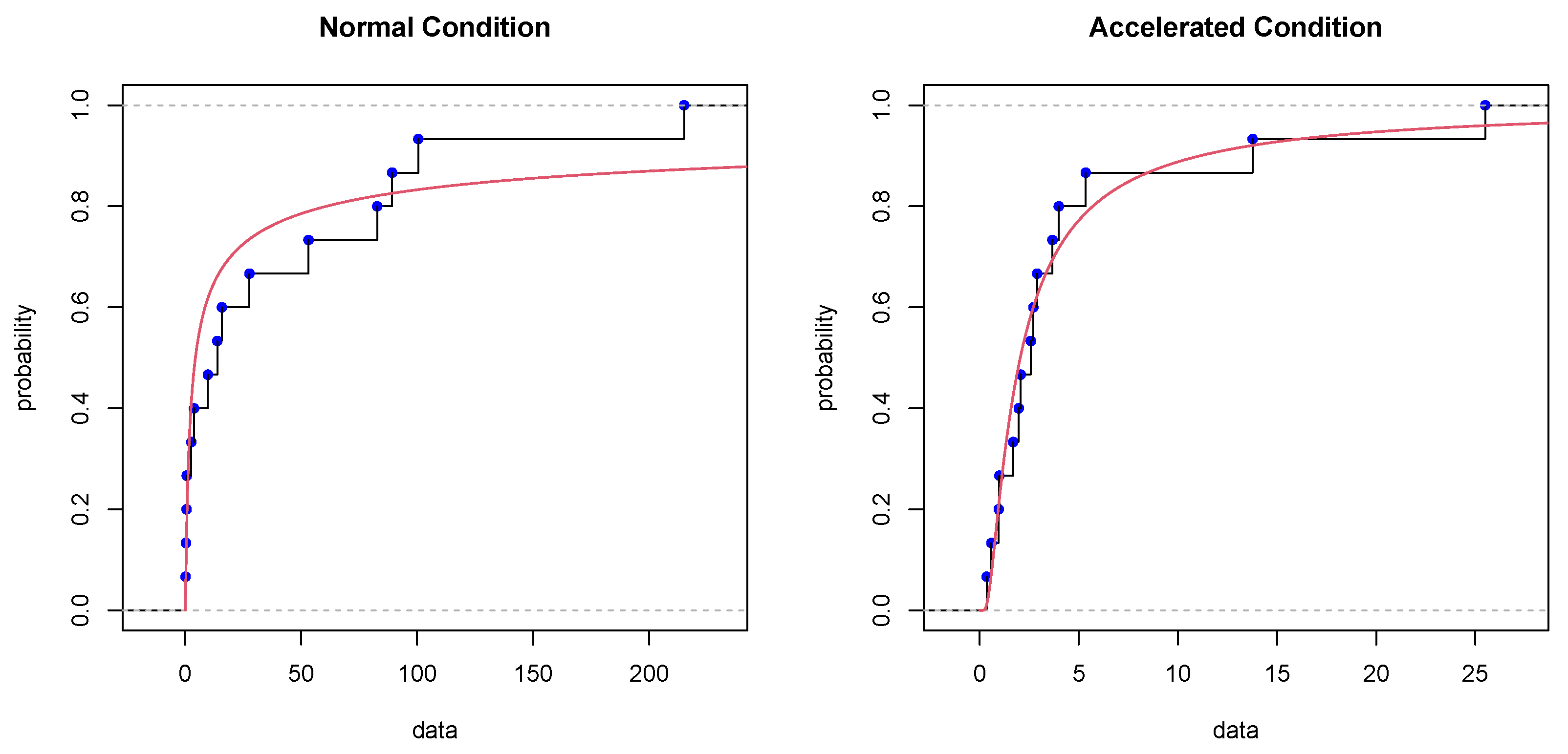
To further demonstrate the appropriateness of the GIED, the Kolmogorov-Smirnov (K-S) test is utilized. The specific samples under two levels of stress (32 KV as normal condition and 36 KV as accelerated condition) is offered in

Table 4. The complete failure data as well as the relevant K-S distances and p-values with 32 KV & 36 KV.

Stress	Failure Times					K-S Distance	p-Value
32 KV	0.27	0.40	0.69	0.79	2.75	0.2180	0.4149
	3.91	9.88	13.95	15.93	27.80
	53.24	82.85	89.29	100.58	215.10
36 KV	0.35	0.59	0.96	0.99	1.69	0.1592	0.7867
	1.97	2.07	2.58	2.71	2.90
	3.67	3.99	5.35	13.77	25.50

. According to the results in Table 3, the data are assumed to follow GIED, thus one can further conduct the K-S test:

$${\mathrm{H}}_0:\mathrm{the}\mathrm{samples}\mathrm{are}\mathrm{from}\mathrm{GIED}vs.{\mathrm{H}}_1:\mathrm{the}\mathrm{samples}\mathrm{are}\mathrm{not}\mathrm{from}\mathrm{GIED},$$

then the corresponding K-S distances as well as p-values are calculated and shown in Table 4 as well. When the p-values are larger than the significance level, one have good reason to accept the null hypothesis, which means determining the samples are from a GIED. Under normal and the accelerated condition, the calculated p-values are $0.4149$ and $0.7867$ respectively, which means that one should accept the null hypothesis ${\mathrm{H}}_0$, leading to a fundamental conclusion that GIED is well-fitting to this dataset. In addition, the empirical cumulative distribution plots of both normal (32 KV) and accelerated (36 KV) condition with the fitted CDF curves where the unknown parameters are given by MLEs are shown in Figure 6, which can be a further illustration of the validity of using GIED model.

Based on Table 4, we generate two new sets of general progressively Type-II censored samples using a specified CS where $n=15,m=12,r=2$ and $R_1=R_2=R_3=1,R_4=\cdots =R_{10}=0$. The new data sets are shown in

Table 5. General progressively Type-II censored samples with CS $n = 15, m = 12, r = 2$ and $R_1 = R_2 = R_3 = 1, R_4 = \cdots = R_{10} = 0$.

Normal condition (32 KV)
0.69	0.79	2.75	9.88	13.95	15.93	27.80	82.85	89.29	100.58
Accelerated condition (36 KV)
0.96	0.99	1.97	2.07	2.58	2.71	3.67	3.99	13.77	25.50

. Hence, one can conduct the classical and Bayesian methods mentioned above on the new data set to derive point and interval estimation of $\alpha$, $\lambda$ as well as $\beta$. For Bayesian methods, because there is no available extra informative knowledge about the three parameters, we set all the hyper-parameters as $0.001$, which indicates that the pre-determined priors are nearly non-informative.

Table 6. Point estimation for $\alpha , \lambda , \beta$ of the censored CSPALT samples.

	$\mathit{\alpha }$	$\mathit{\lambda }$	$\mathit{\beta }$
MLE	0.4661745	1.304002	1.90858
BE	0.4856826	1.356861	2.099287

and

Table 7. Interval estimation for $\alpha , \lambda , \beta$ of censored CSPALT data.

	$\mathit{\alpha }$		$\mathit{\lambda }$		$\mathit{\beta }$
	LB	UB	LB	UB	LB	UB
ACI	0.2229615	0.7093875	0.5894873	2.018516	0.5838548	3.233304
BCI	0.3398963	0.7585613	0.9975824	2.078375	1.167888	2.679973

display the outcomes of different methods, which clearly demonstrate that the effectiveness of MLEs and BEs is highly comparable since they have produced similar estimates of the parameters, whereas for the interval estimation, BCIs works better than ACIs featuring much shorter interval lengths.

Through an analysis of the practical oil breakdown times data set, one can conclude that both classical and Bayesian method are helpful for estimating the parameters of GIED by utilizing general progressively censored samples in a CSPALT, and additionally, Bayesian estimates performed better in terms of the interval lengths.

6. Conclusions

With the modern products becoming more and more durable, researchers have proposed different methods to cut the experimental time and cost, including the accelerated life tests and censoring. This study focuses on combining the CSPLAT and general progressive Type-II censoring to further reduce the time and money cost. Additionally, by adopting GIED (which has a versatile HRF) as the lifetime distribution and utilizing the general censoring methodology, we manage to provide extra flexibility in more complicated situations for the experimenters.

We explore diverse approaches for estimating the parameters of GIED within the framework of a CSPALT based on general progressively censored samples. We delve into both classical and Bayesian perspectives for estimating $\lambda$ and $\alpha$, representing the scale and shape parameter of GIED, as well as the acceleration factor $\beta$. We devise maximum likelihood estimates and provide correlated ACIs by using the Fisher information matrix. Additionally, we derive point and interval estimates through Bayesian methods, leveraging importance sampling for point estimation and establishing Bayesian credible intervals. Monte-Carlo simulations are conducted under multiple censoring schemes to assess the validity and performance of the different methodologies. The results underscore the effectiveness of the mentioned approaches, with Bayesian point and interval estimates demonstrating better performance across most scenarios. The results also reveal the fact that both classical and Bayesian methods are not satisfying enough with small samples, but BEs and BCIs are slightly more effective since they have used the prior information. Finally, the proposed methods are applied on a real lifetime dataset, BCIs outperform the ACIs with shorter interval lengths, justifying that the Bayesian view is more suitable for this dataset, which is consistent with the previous results of the simulation and supports the suitability and applicability of our model.

Moving forward, we aim to extend our investigation to encompass more intricate scenarios, such as step-stress partially accelerated life tests with general progressive Type-II censoring. We remain committed to exploring and developing more effective methods for estimating unknown parameters under diverse scenarios.