A Key Node Mining Method Based on K-Shell and Neighborhood Information

Abstract

Mining key nodes in complex networks has always been a promising research direction in the field of complex networks. Many precise methods proposed by researchers for mining influential special nodes in networks have been widely applied in a plethora of fields. However, some important node-mining methods often use the degree as a node attribute indicator for evaluating node importance, while the clustering coefficient, as an important attribute of nodes, is rarely utilized. Some methods only consider the global position of nodes in the network while ignoring the local structural information of nodes in special positions and the network. Hence, this paper introduces a novel node centrality method, KCH. The KCH method leverages K-shell to identify the global position of nodes and assists in evaluating the importance of nodes by combining information such as structural holes and local clustering coefficients of first-order neighborhoods. This integrated approach yields an enhanced performance compared to existing methods. We conducted experiments on connectivity, monotonicity, and zero models on 10 networks to evaluate the performance of KCH. The experiments revealed that when compared to the collective influence baseline methods, such as social capital and hierarchical K-shell, the KCH method exhibited superior capabilities in terms of collective influence.

1. Introduction

In our interconnected world, complex systems permeate nearly every facet of human society and the natural world, playing indispensable roles in our lives, economies, sciences, and beyond [1,2,3,4,5,6]. Therefore, the understanding, analysis, and prediction of complex systems have attracted the attention of researchers [7]. Every complex system can be abstracted as a complex network, where the objects of the system are viewed as nodes, and the relationships between objects are viewed as edges [8]. The network composed of nodes and edges reveals the interrelationships between different parts of the complex system. For example, the power system that provides energy to the world is composed of generators and transmission lines [9]. The biological network, which is a necessary condition for life, is composed of cells and their interactions [10]. The social network that dictates the dissemination of knowledge and resources in society is made up of relationships between individuals, such as family, friends, and professional connections [11]. Due to the heterogeneity of complex networks, certain “special nodes” in the network have significant influence [12]. Operating on these “special nodes” often has a significant impact on the network [12], and these “special nodes” are referred to as key nodes. Therefore, key node mining in complex networks has been widely applied in many fields [13], such as the prevention of infectious diseases [14], viral marketing [15], and prevention of social network rumors [16].

As one of the important research directions in complex networks, important node mining has been proposed by many researchers [17]. Among these methods, the centrality-based methods are the main category, and the important node-mining methods based on centrality can be divided into three types: local indicators, global indicators, and semi-local indicators [18]. Alternatively, these methods can be categorized into centrality methods relying on local information and centrality methods based on global information. Within this classification, the centrality methods based on local information encompass both local indicators and semi-local indicators. The distinction between the two lies in their scope: local indicators solely consider the node and its immediate neighbors, whereas focusing solely on the node and its first-order neighbors often yields less precise results and greater limitations. Therefore, semi-local indicators not only consider the node and its first-order neighboring nodes but also consider higher-order neighboring nodes. Degree centrality (DC) stands as the quintessential method grounded in local indicators, which posits that a node’s significance increases with its degree [19]; the social capital (SC) method, proposed by Zhou et al., suggests that a node’s importance correlates with the sum of its degree and that of its immediate neighbors [20]; the semi-local centrality (SLC) method, proposed by Chen et al., mirrors SC by evaluating the importance of a node by the sum of the degrees of the node and its neighbors [21], albeit with the distinction of incorporating information from the node’s higher-order neighbors. In addition to the aforementioned methods that assess the importance of nodes based on their degree, there are other centrality methods based on local information, such as the H-index method, which was initially used to evaluate academic output and was applied to the field of complex networks by Lue et al. [22]; and Zareie et al. proposed the entropy-based ranking measure (ERM), which introduces information entropy theory and evaluates the importance of nodes by combining different disciplinary knowledge [23]. In comparison, centrality methods based on global information have the capacity to incorporate more extensive data. For instance, closeness centrality (CC) [24] and betweenness centrality (BC) [25] are classic centrality methods based on global information. However, they may not be very suitable for large-scale networks due to their intricate computations and high time costs [21]. The K-shell (KS), proposed by Kitsak et al., can quickly rank the importance of nodes in a network and is suitable for large-scale networks [26]. This method categorizes nodes based on their degrees, thus identifying whether a node serves as a core within the network. While this approach heralds a novel measurement paradigm, it introduces a significant issue of monotonicity, whereby it fails to discern variations in node importance within the same stratum. To address this, researchers have proposed a series of improved methods, such as extended coreness centrality (CNC+) [27], classified neighbors (CN) [28], KSIF [29], and mixed degree decomposition (MDD) [30], among others.

Traditional methods for mining important nodes often rely on the degree as the core criterion for assessing node importance. While this intuitive approach is effective and yields significant results, the degree alone does not fully capture a node’s importance. Nodes with a low degree can also play crucial roles in the network. For example, bridge nodes that connect different communities may have a small degree, but they have a high level of influence and are undeniably important. Additionally, the clustering coefficient, another vital attribute of a node, is seldom utilized in existing methods for mining important nodes [31].

Therefore, this paper introduces an innovative method for identifying key nodes in the network based on K-shell and node neighborhood information, called KCH. KCH posits that the importance of a node in the network is determined by both the node’s own information and the node’s neighborhood information. The individual information of a node is represented by the KS value, while the neighborhood information of a node is determined by the combined local clustering coefficient and structural hole coefficient of its adjacent nodes. The time complexity of the KCH method is $O\left(\overline{n}·\left|E\right|\right)$, where $\overline{n}$ is the average degree of the network, and $\left|E\right|$ is the number of edges in the network. Below are the main advantages of our proposed KCH:

(1)

KCH adopts a hybrid approach to integrating both global and local information. The KCH method enhances the traditional K-shell approach by incorporating comprehensive network information. It combines structural hole data and the local clustering coefficient—an essential node attribute—with local topological structure information.

(2)

The experimental results on connectivity, monotonicity, and null models across ten networks demonstrate that KCH outperforms other K-shell variant methods and non-K-shell variant methods such as collective influence (CI), SC, hierarchical K-shell (HKS). The KCH shows superior accuracy, monotonicity, and universality, effectively identifying the influence of a node within the network.

The remainder of this paper is organized as follows: Section 2 of the paper reviews related work on important node mining. Section 3 introduces the baseline methods and the specific details of the KCH method proposed in this paper. Section 4 describes the experiments conducted to evaluate the performance of KCH, analyzes the experimental results, and assesses the effectiveness of the KCH method. Finally, Section 5 summarizes the key findings of the paper.

2. Related Works

Since the inception of complex networks, industry professionals have continuously sought to attempt to uncover “special nodes” within the network. When these “special nodes” are either destroyed or strengthened, they significantly impact the paper. These “special nodes” are referred to as key nodes, and identifying them has been a fundamental research challenge in complex network analysis. Centrality methods have proven highly effective in locating these key nodes within the network [32].

2.1. Local Indices

Local index-based centrality methods often assess the node’s importance by collecting information from the node’s neighborhood. Examples include DC, H-index, and SC. DC is centered around the degree, positing that a node’s importance increases with the number of its neighbors [19]. Although this algorithm is simple, it has a fatal flaw: it only considers the number of adjacent nodes and ignores edge weights, which restricts its performance in weighted networks. The H-index, extended to complex networks by Lv and colleagues, measures a node’s importance through the degree of its neighbors [22]. SC, proposed by Zhou et al., evaluates the importance of a node by the sum of the node’s degree and the degrees of its neighbors [20].

Focusing solely on a node and its first-order neighbors often lacks precision and has significant limitations. Therefore, methods that consider a node’s local information without being restricted to the nearest neighbors have been widely proposed. Such methods are referred to as semi-local index-based centrality methods; for example, SLC, local structural centrality (LSC), ERM, and Spon. SLC, proposed by Chen et al., follows a rationale similar to SC, measuring the importance of a node by the sum of the degrees of the node and its neighbors [21]. However, SLC fully utilizes the information of the node’s higher-order neighbors, whereas SC only uses the degree information of the first-order neighbors. Zhao et al. proposed Spon, which measures the importance of a node by calculating the “neighbor ratio” of a node’s neighbors. The “neighbor ratio” refers to the ratio of the number of a node’s first-order to its second-order neighbors, essentially still using the degree to measure the importance of a node [33]. Unlike the aforementioned methods that rely solely on degree, Gao et al. proposed LSC, which takes into account both the degree of a node and its topological information [34]; Zariee et al. proposed ERM, incorporating the concept of entropy from information theory into node centrality, assessing the importance of a node based on the information entropy of the node and its first-order and second-order neighbors [23].

Most of the aforementioned methods are degree-based, but a node’s degree is not necessarily indicative of its importance [27]. The term “structural hole” originates from social network research [35]. In networks, structural hole nodes serve as bridges or connectors between different communities within the network. Monitoring structural hole nodes can effectively curb the spread of rumors, and these nodes have advantages in information dissemination, innovation, and resource integration [36,37]. If structural hole nodes are removed, different communities within the network become disconnected; thus, structural hole nodes often have a low degree but possess significant importance.

Local index-based centrality methods only utilize the local neighborhood information of a node (i.e., information between the node and its neighbors) to rank the importance of the node. These methods are advantageous due to their computational simplicity and high efficiency, making them suitable for large- and medium-sized networks. However, they struggle to assess node importance from a holistic perspective and find it difficult to measure the true importance of nodes such as structural holes.

2.2. Global Indices

Global index-based centrality methods measure the influence of a node according to the overall topological structure of the network. Examples include CC, BC, and the K-shell method. CC measures the average shortest path distance between a target node and other nodes, essentially being the inverse of the average shortest path distance from the node to others [24]. BC assesses a node’s importance by counting the number of shortest paths that pass through it [25]. However, both CC and BC have significant drawbacks: they are computationally complex and not suitable for large networks [21]. In contrast, the K-shell method is a fast-computing and large-network-appropriate method for mining important nodes, proposed by Kitsak et al. [26]. The K-shell method distinguishes the importance of nodes by stratifying them according to their degree; nodes with higher K-shell values are considered more important. The time complexity of the K-shell is relatively low at O(E), where E is the number of edges in the network [38].

However, the KS method has a significant limitation; it cannot assess the difference in importance among nodes of the same layer. To address the monotonicity issue, researchers have proposed several improved methods, including CNC+, CN, KSIF, and MDD. The CNC+ method posits that the importance of a node should be determined by combining the KS values of neighboring nodes [27]. The CN method suggests that the order in which nodes are removed by the KS method affects the assessment of node importance and should be combined with its KS value to evaluate node significance [28]. The KSIF method assesses node importance through the iterative information of node removal [29]. The MDD method argues that assessing the importance of a node requires considering both the edges of the removed node and the edges of the remaining nodes [30].

In addition to these methods, PageRank, a centrality method based on random walks, also falls into the category of global index-based centrality methods. Originally used for web page ranking, PageRank assesses the importance of a web page by considering both the number and quality of a web page [39]. LeaderRank, a variant of PageRank, is another classic centrality method based on random walks. However, these two methods perform poorly in undirected networks and are more commonly used in directed networks [21]. De Arruda and colleagues have demonstrated through experiments that reachability is the best centrality indicator for measuring the importance of nodes in spatial networks with topological constraints [26].

Global index-based centrality methods often achieve higher computational accuracy compared to local index-based centrality methods. This is because they consider the overall topological structure of the network, and using more comprehensive information leads to more precise results. However, this approach also has disadvantages: the computational complexity is typically higher and more time-consuming, making it difficult to apply these methods to large-scale networks.

2.3. Hybrid Methods

Hybrid methods often employ a combination of local and global information to measure a node’s influence, leveraging the strengths of both approaches. For instance, local-and-global centrality (LGC), proposed by Ullah et al., integrates local and global centrality metrics, considering the network’s topology to identify key nodes [40]. Similarly, improved K-shell (IKS), proposed by Wang et al., merges K-shell analysis with node information entropy to rank nodes based on both their local and informational significance [41]. K-shell based on gravity centrality (KSGC), an enhancement over the local version of GM (LGM) by Yang et al., incorporates node positional data and degree disparities to differentiate node importance [42]. Additionally, the extended K-shell hybrid method (KS+), as proposed by Amrita et al., evaluates node importance by comprehensively considering the K-shell, degree, contact distance, and the extent of neighborhood influence [32]. Although these hybrid methods outperform single-method approaches by incorporating diverse criteria, they may still overlook influential nodes on the network’s periphery. This highlights a potential area for further development or refinement in hybrid methodologies to capture the significance of such nodes effectively.

Zhao [43] proposed a hybrid method named Mixedinf, which considers a node’s degree, its neighbors, and structural holes (SH) to determine its importance. The method acknowledges that different nodes contribute differently to the importance assessment, and it uses hyperparameters to balance the contributions of degree and SH. Zhao emphasized that the contributions of degree and SH vary and thus need careful consideration. Tang et al. proposed a centrality method called semi-local centrality and structural holes (LSH), which combines SH with the modified local centrality (MLC) method to better evaluate the importance of bridging nodes and core nodes with multiple neighbors [44]. The MLC method, proposed by Zhao et al. [45], is an improved local centrality approach that considers the order of a node’s neighbors based on expansion frequency. They argue that nodes with higher expansion frequencies wield greater influence, necessitating comprehensive consideration of the neighbor order. Both the Mixedinf and LSH methods incorporate SH into their criteria for measuring node importance, thereby enabling the recognition of influential spreaders, even among peripheral nodes in the network. These hybrid approaches, leveraging both global and local information, address some limitations inherent in purely global or local centrality methods. Consequently, this study adopts a hybrid strategy to enhance the KS method by incorporating the network’s local structural information.

3. Proposed Methods

In this paper, we propose a novel approach for mining key nodes in a network termed KCH, which represents an enhancement over the K-shell method. KCH integrates both the local clustering coefficient and the concept of SH. Unlike some related methods, KCH effectively resolves the monotonicity issue inherent in the K-shell method. Moreover, it demonstrates superior capability in identifying core nodes compared to other methods designed to enhance the K-shell approach. Notably, KCH performs competitively with several outstanding non-K-shell variant methods.

3.1. Baseline Methods

3.1.1. Collective Influence (CI)

The collective influence (CI) metric, introduced by Morone and Makse [46], serves as an indicator to evaluate node importance within a network. This metric assesses a node’s influence based on the impact on the giant connected component following its removal. The CI of node i is calculated as follows:

$$C{I}_i=\left(d_i-1\right) {{\displaystyle \sum }}_{j\in \partial N\left(i,l\right)}\left(d_j-1\right)$$

(1)

Here,${\mathrm{d}}_{\mathrm{i}}$ represents the degree of node $\mathrm{i}$, and $\mathrm{N}\left(\mathrm{i},\mathrm{l}\right)$ denotes the set of nodes comprising all nodes on the circle centered at node $\mathrm{i}$ with a length radius of $\mathrm{l}$. The value of $\mathrm{l}$ is arbitrarily defined and varies depending on the network size. Typically, for smaller networks, $\mathrm{l}$ is set to 2, while for larger networks, it is set to 3.

3.1.2. Social Capital (SC)

The social capital (SC) metric, introduced by Zhou et al. [20], is a local centrality measure designed to evaluate node influence within complex networks. SC suggests that a node’s influence is determined by both its own degree and the degrees of its neighboring nodes. The SC of node i is defined as follows:

$$S{C}_i=d_i+{\displaystyle \sum }_{j\in V_i}{d}_j$$

(2)

In the formula, ${\mathrm{d}}_{\mathrm{i}}$ represents the degree of node $\mathrm{i}$, ${\mathrm{V}}_{\mathrm{i}}$ represents all neighboring nodes of node $\mathrm{i}$, and ${\mathrm{d}}_{\mathrm{j}}$ represents the degree of neighbor node $\mathrm{j}$ of node $\mathrm{i}$.

3.1.3. Hierarchical K-Shell (HKS)

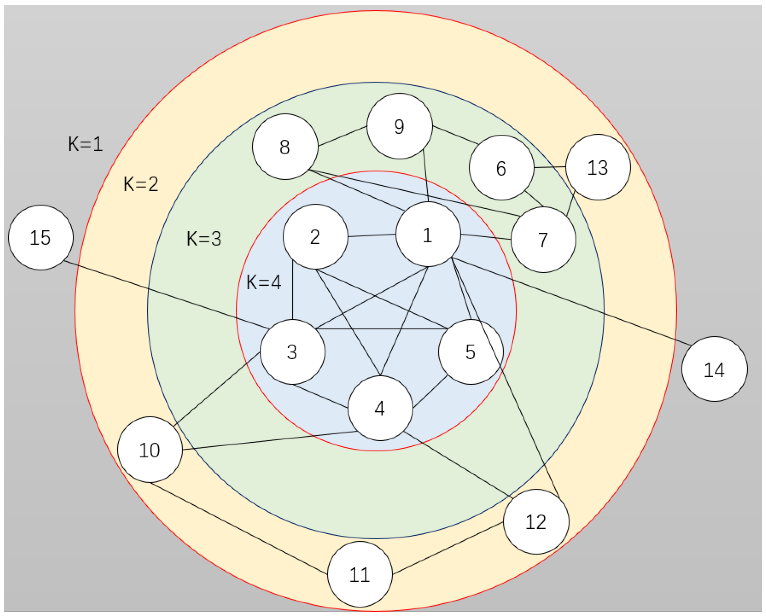
The hierarchical k-shell (HKS), proposed by Ahmad Zareie and Amir Sheikhahmadi, is a method for identifying influential spreaders in complex networks. They argue that a node’s topological position and its proximity to the core of the network play significant roles in determining its importance. The HKS method estimates a node’s spreading capability based on the node’s position and degree, as well as the position and degree of adjacent nodes [47]. It is defined as follows:

$$HKS\left(v_i\right)={\displaystyle \sum }_{v_j\in N\left(v_i\right)}S\left(v_j\right)$$

(3)

Here, ${\mathrm{v}}_{\mathrm{i}}$ represents the current node and $N\left(v_i\right)$ denotes the set of neighboring nodes of the current node. The definition of $\mathrm{S}\left({\mathrm{v}}_{\mathrm{i}}\right)$ is as follows:

$$S\left(v_i\right)={\displaystyle \sum }_{v_j\in N_i}{d}_j+\left(b_j+f_j\right)$$

(4)

Here, ${\mathrm{v}}_{\mathrm{i}}$ represents the current node, ${\mathrm{N}}_{\mathrm{i}}$ denotes the set of neighboring nodes of the current node, ${\mathrm{d}}_{\mathrm{j}}$ indicates the degree of the adjacent node, ${\mathrm{b}}_{\mathrm{j}}$ is the distance from the node to the network periphery (indicating the node’s degree of being far from the periphery), and ${\mathrm{f}}_{\mathrm{j}}$ is the distance from the node to the network core (indicating the node’s degree of being close to the core).

3.1.4. K-Shell (KS)

K-shell is a global index-based centrality technique proposed by Kitsak et al. [26] for rapidly identifying the importance of nodes in a network based on their proximity to the core layers. This method is efficient, with low time complexity, making it suitable for large-scale networks. However, it struggles to accurately differentiate the importance of nodes within the same stratum.

The main steps of the KS method involve recursively removing nodes with degrees ranging from 1 to k. The process begins by categorizing isolated nodes with a degree of 0 as the 0-shell. Next, nodes with a degree of 1 are removed. This removal may cause new nodes to have a degree of 1 due to the disconnection of edges, and these nodes are also removed. This process continues until no nodes with a degree of 1 remain. The removed nodes are assigned a K-shell (KS) value of 1 and are categorized as the 1-shell. The procedure is then repeated for nodes with degrees from 2 up to k, assigning corresponding KS values to each group of removed nodes until every node in the network has been assigned a KS value.

3.1.5. Closeness Centrality (CC)

Closeness centrality (CC) is one of the classic methods for mining important nodes. CC considers the average length of the shortest paths from each node to all other nodes [25]. CC posits that if a node is of high importance, it is close to other nodes. The advantage of this method is its high accuracy, while the disadvantage is its high computational cost, making it unsuitable for large-scale networks. The definition of CC is as follows:

$$C{C}_i=\frac{\left|V\right|-1}{{{\displaystyle \sum }}_{j\ne i}{d}_{ij}}$$

(5)

Here, $d_{ij}$ represents the distance of the shortest path from node $i$ to node $j$.

3.1.6. Extended Coreness Centrality (CNC+)

The extended coreness centrality method (CNC+) is an improvement based on the K-shell method proposed by Bae et al. [27]. CNC+ posits that the importance of a node should be jointly determined by the KS values of first-order and second-order neighboring nodes. CNC+ is defined as follows:

$$CN{C}_{+}\left(i\right)={\displaystyle \sum }_{v_j\in N_i}CNC\left(j\right)$$

(6)

$$CNC\left(j\right)={\displaystyle \sum }_{v_j\in N_i}k{s}_j$$

(7)

In the formula, $N_i$ represents the set of neighboring nodes of node i and $k{s}_j$ indicates the ks value of the neighbor node j of node i.

3.2. KCH Methods

3.2.1. Clustering Coefficient

The clustering coefficient is a crucial concept in graph theory, used to understand the relationships between nodes in a network and their organizational characteristics. The local clustering coefficient of a node measures the closeness of connections between its neighbors. Specifically, it quantifies the closeness of connections between a node’s neighbors [31]. The local clustering coefficient of node $i$ is the ratio of the actual number of edges between node $i^{\prime }$s neighbors to the maximum possible theoretical number of edges between node $i^{\prime }$s neighbors, as follows:

$$C_i=\frac{2E}{n\left(n-1\right)}$$

(8)

Here, $n$ is the number of neighboring nodes of node i and $E$ is the number of edges that truly exist between the neighbors of node i.

3.2.2. Structural Hole

Structural holes refer to nodes or groups of nodes in a network that act as bridges, connecting different communities. These nodes, even if they have a low degree, can be crucial due to their strategic positions within the network [48]. For example, the position of structural hole nodes in the network allows them to obtain information and resources from multiple groups; this is conducive to eliminating barriers between different communities and promoting cooperation and communication across groups. To measure the control of structural hole nodes over various relationships in the network, Burt proposed the network constraint coefficient [37], defined as follows:

$$S{H}_i={\displaystyle \sum }_j{\left({\mu }_{ij}+{\displaystyle \sum }_{k\ne i,j}{\mu }_{ik}{\mu }_{kj}\right)}^2$$

(9)

In the formula, node $k$ is a common neighbor of nodes i and j, and ${\mu }_{ij}$ represents the proportion of effort that nodes i and j invest in maintaining their relationship compared to the total effort of node i. This is defined as follows:

$${\mu }_{ij}=\frac{e_{ij}}{{{\displaystyle \sum }}_{j\in N_i}{e}_{ij}}$$

(10)

Here, $N_i$ represents the set of neighboring nodes of node i. If $e_{ij}=1$, there is an edge between i and j, and if $e_{ij}=0$, there is no edge. The constraint coefficient measures a node’s position in the network and the tightness of its connections, describing the connectivity between a node and its neighbors. A node with a smaller constraint coefficient has more connections and a brokering position in the network, enabling it to control the flow of information and distribution of resources within structural holes. This is because such a node can access information from different subgroups and mediate communication and exchange between these subgroups.

3.2.3. KCH

Consider a simple undirected, unweighted graph $G\left(V,E\right)$, where $V$ represents the set of nodes, and $E$ is the set of edges. In many networks, nodes with a low degree can also be influential; for example, bridge nodes with SH are typical low-degree, high-influence nodes. Additionally, a higher local clustering coefficient indicates that a node’s neighbors tend to cluster together, which can enhance the node’s influence. Therefore, this paper uses the KS method to collect the global topological structure information of the network while also obtaining local structural information through SH and the clustering coefficient. By combining both global and local structural information, we aim to measure and rank the importance of nodes more effectively. The KS method, which has been detailed in Section 3.1, will not be reiterated here in Section 3.2.

The first-order clustering coefficient of node i is defined as the sum of the local clustering coefficients of its first-order neighbors. Let $N_i$ represent the set of neighboring nodes of node i. The specific definition is as follows:

$$C_i^1={\displaystyle \sum }_{j\in N_i}{C}_j$$

(11)

Since node i is also a neighbor to its first-order neighbors, it affects the calculation of the first-order clustering coefficient. Furthermore, the smaller the network constraint coefficient of a node, the higher the likelihood of it being a structural hole, indicating stronger influence capability. In this method, we use the reciprocal of the network constraint coefficient to measure the SH evaluation, as shown in the following formula, where a larger SH value signifies stronger influence capabilities.

$$s{h}_i=\frac{1}{S{H}_i}$$

(12)

The calculation method of KCH involves two primary steps. First, we use the K-shell algorithm to obtain the KS values, $k{s}_i,$ for each node in the network G. Then, we calculate the structural holes ($s{h}_i)$ and the first-order clustering coefficient ($C_i^1$) for each node using the aforementioned formulas. Second, we calculate the KCH value for each node.

The KCH centrality of a node is defined by the following formula:

$$KCH\left(i\right)=k{s}_i+y_i$$

(13)

$$y=f\left(sh+C^1\right)$$

(14)

$$f\left(x\right)=\frac{x-min}{max-min}$$

(15)

Here, $f()$ represents the maximum–minimum normalization formula, y is the normalized data result, x is the original data, and $min$ and $max$ denote the minimum and maximum values of the original data, respectively. A higher KCH value indicates greater importance of the node.

We use the example network to illustrate the execution process of the KCH method. The network has 15 nodes and 27 edges, and its K-shell layered diagram is shown in Figure 1. We initiate the demonstration of the KCH by selecting node 3 as an example to showcase its execution process.

First, we calculate the $k{s}_i$ (values of K-Shell) of node 3, which is 4. Next, we identify the neighboring nodes of node 3, which are its closest neighbors: 1, 2, 4, 5, 10, and 15.

Next, we calculate the local clustering coefficient and network constraint coefficient for each neighboring node. Subsequently, we compute the $C_i^1$ and $s{h}_i$ of node 3, and calculate the sum of the two, which is 5.7660. Then, normalize it. The local clustering coefficient and network constraint coefficient of the first-order neighbors of node 3 are shown in

Table 1. The local clustering coefficient and network constraint coefficient of the first-order neighbors of node 3 in the example network.

Node	1	2	4	5	10	15
local clustering coefficient	0.25	1	0.53	1	0	0
network constraint coefficient	0.2496	0.5788	0.4179	0.5788	0.9999	0.5000

.

Finally, we obtain the KCH value of this node by adding its $k{s}_i$ and the $y_i$.

$$KCH\left(i\right)=k{s}_i+y_i=k{s}_i+f\left(s{h}_3+C_3^1\right)=4+f\left(5.7660\right)=4.6083$$

(16)

The time complexity of the KCH method is primarily concentrated in two parts. The first part involves the calculation of KS values, structural holes, and the first-order clustering coefficient. The second part is the calculation of KCH itself. The K-shell algorithm requires traversing each node and edge in the graph, resulting in a time complexity of $O\left(\left|V\right|+\left|E\right|\right)$, where $\left|V\right|$ is the number of nodes in the network and $\left|E\right|$ is the number of edges. Calculating structural holes and clustering coefficients requires considering the first-order neighbors of a node and the edges connected to them, leading to a time complexity of $O\left(\overline{n}·\left|E\right|\right)$, where $\overline{n}$ is the average degree of the network. The calculation of the KCH value is only related to the number of nodes, resulting in a time complexity of $O\left(\left|V\right|\right)$. Given that the number of edges in a network is typically much higher than the number of nodes and the average degree of nodes, the overall time complexity of the KCH method is $O\left(\overline{n}·\left|E\right|\right)$.

4. Experiments and Results

4.1. Datasets

In our study, we conducted experiments using 10 empirical networks to test the performance of KCH and the baseline methods. These empirical networks, which come from different real-life domains, include HepPh (social network), UspowerGrid (power grid network), Health (healthcare network), C_ElegansNeural (biological network), Dolphins (dolphin social network), Windsurfer (social network), Seventh (social network), Tribes (social network), Rhesus (rhesus social network), and WikiVote (social network). Details of the networks are shown in

Table 2. Basic topological features of network data. The leftmost column presents the names of the networks, $N$ and $E$ represent the number of nodes and edges in the network; <K> and $K_{max}$ represent the average degree and maximum degree of the network; $C$ and $r$ indicate the global clustering coefficient and assortativity coefficient of the network.

Networks	N	E	<K>	Kmax	C	r
Windsurfer	43	336	15.63	31	0.6534	−0.147
WikiVote	889	2914	6.56	102	0.1528	−0.0288
USpowerGrid	4941	6594	2.67	19	0.0801	0.0035
Tribes	16	58	7.25	10	0.5392	0.0499
Seventh	29	250	17.24	28	0.7767	−0.1575
Rhesus	16	69	8.63	12	0.7085	−0.1091
HepPh	11,204	117,619	19.00	491	0.6115	0.6323
Health	2539	10,455	8.24	27	0.1467	0.2513
Dolphins	62	159	5.13	12	0.259	−0.0436
C_ElegansNeural	297	2148	14.46	134	0.2924	−0.1632

.

4.2. Metrics

4.2.1. Robustness Metrics

Connectivity tests serve as a reliable method for assessing the significance of nodes and are a classic approach for gauging their importance. During experiments, we commonly employ important node-mining algorithms to rank the importance of nodes in the network. Subsequently, nodes are systematically removed, commencing with the most crucial ones. If the network undergoes substantial deterioration following the removal of a node, that node is deemed important. The robustness indicator R, often used to assess the degree of network degradation [49], is defined as follows:

$$R=\frac{1}{N}{\displaystyle \sum }_{i=1}^{N}r\left(i\right)$$

(17)

In this formula, 1/N represents the normalization factor, while r(i) indicates the change in the network after the removal of node i. Specifically, it reflects the ratio of the size of the largest connected component post-removal of node i to the total number of nodes in the network after the removal. R represents the area under the curve formed by the r(i) values plotted against Cartesian coordinates. A rapid decline in r(i) upon the removal of crucial nodes signifies severe network impairment. Consequently, higher accuracy in node importance mining corresponds to a smaller R-value.

4.2.2. Monotonicity

Accurately discerning the impact of each node constitutes a fundamental challenge for important node-mining algorithms, with monotonicity serving as a pivotal metric for this assessment. The KS method has significant problems with monotonicity, often judging many nodes to have consistent importance, which is a manifestation of low monotonicity. Hence, this paper uses the monotonicity metric M to evaluate the monotonicity of KCH. The definition of the ranking monotonicity M is as follows [50]:

$$M={\left[1-\frac{{{\displaystyle \sum }}_{i\in L}{n}_i\left(n_i-1\right)}{\left|V\right|\left(\left|V\right|-1\right)}\right]}^2$$

(18)

In the formula, $\left|V\right|$ represents the number of nodes in the network, $L$ is the ranking result generated by the algorithm, and $n_i$ denotes the number of nodes with rank $i$ in the result. The monotonicity is strongest when $M=1$, and the monotonicity is worst when $M=0$.

4.3. Performance of KCH

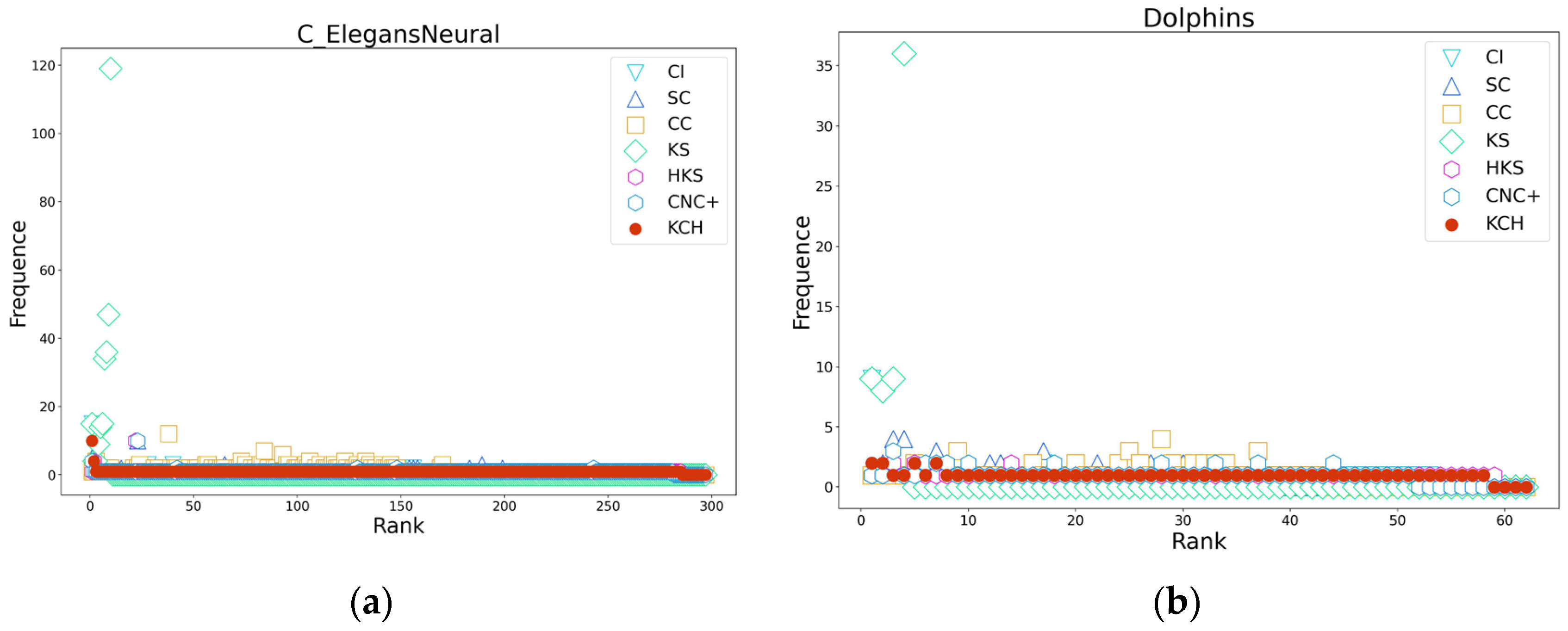
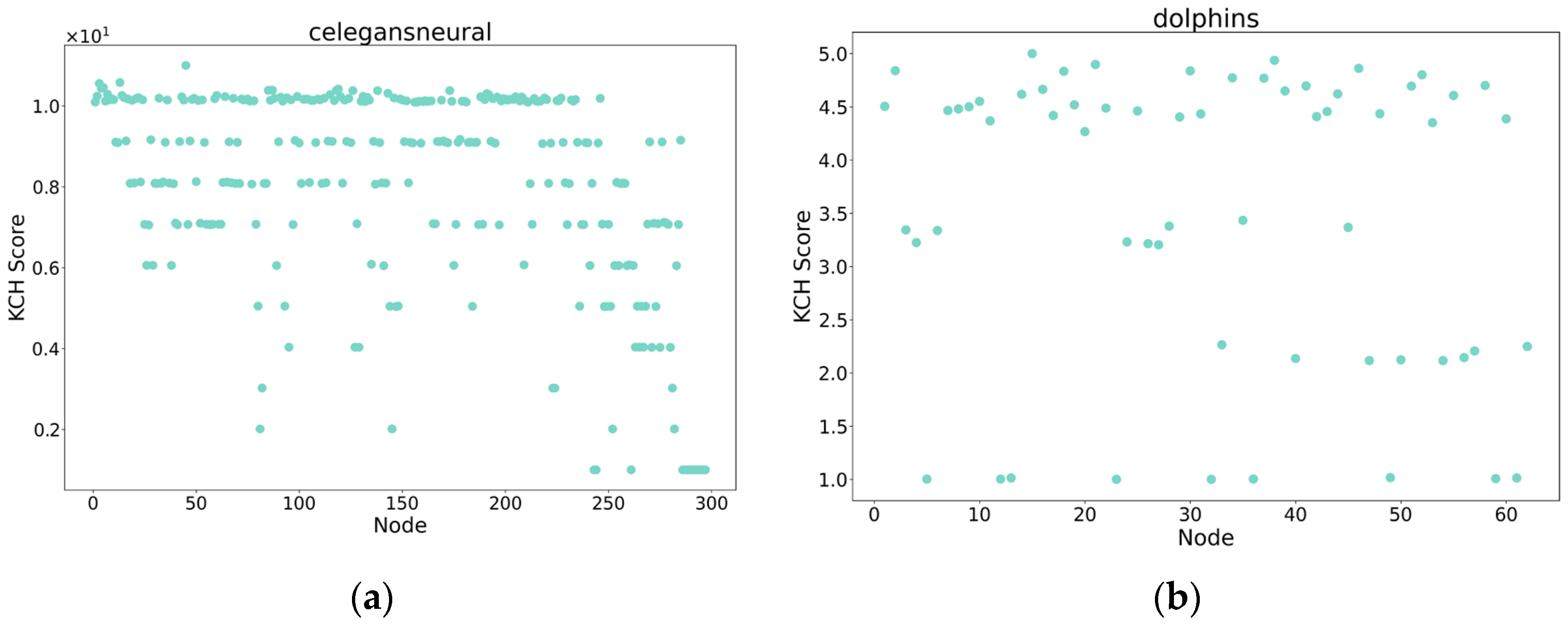
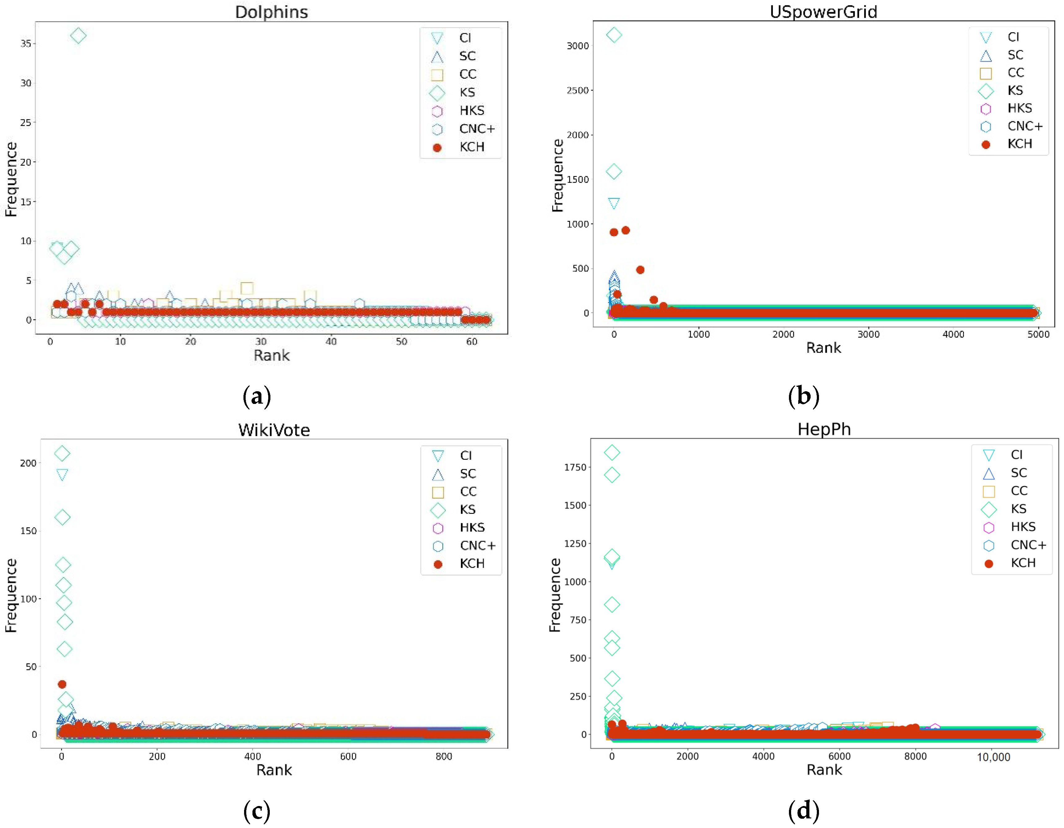
4.3.1. Connectivity Analysis

In this paper, method accuracy is measured by the changes in robustness and the values of the robustness indicator R during the process of node removal in experiments. The accuracy performance of KCH in the Dolphins, USpowerGrid, WikiVote, and HepPh networks is shown in Figure 2, while the accuracy performance of all networks is displayed in Appendix A.

To gauge the accuracy of the algorithm, node rankings are generated using KCH and baseline methods, followed by sequential network destruction. Figure 2 and Appendix A visually display the destruction process of 10 real-world networks. In each experiment, the node’s importance is initially assessed using KCH and benchmark methods. Nodes are ranked based on these assessments, and network destruction begins with the most important node. The robustness indicator R-value is then calculated based on the destruction outcomes, with the method’s accuracy measured accordingly. From the results shown in Figure 2, the change curve of KCH generally resides at the lower end in nine networks, with the area formed by the curve, the x-axis, and the y-axis being the smallest. This suggests that in these nine real networks, deleting nodes according to the node importance ranking generated by KCH leads to the fastest destruction of the network. In essence, the KCH method can destroy the network more quickly than other methods, which indicates that the KCH method can more accurately mine important nodes.

Table 3. Robustness indicator R-values of various centrality metrics on different datasets, with the method having the smallest R-value highlighted in bold.

Networks	KCH	CI	SC	HKS	KS	CC	CNC+
Windsurfer	0.4170	0.4191	0.4240	0.4283	0.4294	0.4310	0.4240
WikiVote	0.2052	0.2188	0.2419	0.2799	0.2200	0.2954	0.2638
USpowerGrid	0.0826	0.0876	0.0915	0.1000	0.2113	0.1973	0.1179
Tribes	0.4219	0.4375	0.4375	0.4414	0.4375	0.4297	0.4375
Seventh	0.4578	0.4602	0.4661	0.4637	0.4649	0.4602	0.4661
Rhesus	0.4063	0.4141	0.4102	0.4141	0.4375	0.4141	0.4141
HepPh	0.2727	0.2693	0.2868	0.3323	0.2814	0.2851	0.3270
Health	0.4195	0.4202	0.4281	0.4514	0.4437	0.4353	0.4376
Dolphins	0.2789	0.2882	0.3184	0.3387	0.2968	0.3699	0.3215
C_ElegansNeural	0.3464	0.3480	0.3869	0.3722	0.3902	0.3942	0.3869

comprehensively shows the comparison of R-values of various methods in 10 real network datasets, with KCH having the smallest R-value in 9 datasets and the second smallest in 1 dataset. Overall, in terms of important node mining, the KCH method demonstrates superior performance.

4.3.2. Monotonicity Analysis

In this paper, we utilize the monotonicity metric M and rank distribution graphs to evaluate the monotonicity of the methods. In the rank distribution graph, the horizontal axis represents the rank of the nodes, while the vertical axis indicates the number of nodes with the same rank. To assess whether an algorithm exhibits good monotonicity in the graph, we examine its rank distribution curve; the closer the curve lies to the bottom of the graph as a straight line, the better the algorithm’s monotonicity.

Table 4. Comparison of monotonicity M-values of various centrality metrics across different datasets, with the method having the highest M-value highlighted in bold. The last row in red font shows the average monotonicity results, and the leftmost column in blue font presents the monotonicity results for KCH.

Networks	KCH	CI	SC	HKS	KS	CC	CNC+
Windsurfer	1.0000	0.9824	0.9956	1.0000	0.4269	0.9454	1.0000
WikiVote	0.9958	0.9100	0.9887	0.9997	0.7265	0.9988	0.9976
USpowerGrid	0.8417	0.8646	0.9048	0.9963	0.2460	0.9998	0.9419
Tribes	1.0000	0.8867	0.9834	1.0000	0.0156	0.7951	1.0000
Seventh	0.9951	0.8622	0.9902	1.0000	0.1365	0.8622	0.9951
Rhesus	1.0000	0.7656	0.9669	1.0000	0.3501	0.7656	1.0000
HepPh	0.9994	0.9798	0.9941	0.9998	0.8350	0.9995	0.9991
Health	0.9997	0.9982	0.9894	0.9999	0.5245	0.9994	0.9979
Dolphins	0.9958	0.9613	0.9675	0.9968	0.3769	0.9737	0.9873
C_ElegansNeural	0.9977	0.9949	0.9955	0.9977	0.6094	0.9893	0.9975
Average	0.9825	0.9206	0.9776	0.9990	0.4247	0.9329	0.9917

presents the results of the monotonicity M-values for different methods.

From the aforementioned results, it is evident that the KS method exhibits the worst monotonicity, while KCH, HKS, and CNC+ exhibit the best monotonicity. Among these methods, HKS has the highest average monotonicity, closest to 1, followed by CNC+ and then KCH. However, the average monotonicity of KCH only differs from CNC+ by 0.0092 and from HKS by 0.0165.

The HKS method estimates the node’s importance based on node position, degree, and the characteristics of neighboring nodes, while CNC+ assesses the node’s importance by considering the degree of neighboring nodes and KS values. While these methods offer high monotonicity, they also come with drawbacks. The HKS method exhibits very high time complexity, making it challenging to apply in large networks. For example, in the HepPh network, when implementing the algorithm on the same computer with the same programming language and style, the HKS method takes up to 2756 s of CPU time, while the KCH method only takes 24 s, with the complex importance calculation of HKS bringing a hundredfold increase in time cost. Additionally, the HKS and the CNC+ methods may overlook important information when assessing the importance of nodes, and their accuracy may not match that of the KCH.

The reason KCH possesses extremely high monotonicity stems from its combination of global network information and local structural information to jointly assess the importance of nodes. As long as two nodes do not have completely identical neighbor structures and the same KS levels, KCH can distinguish the importance of different nodes. The slightly lower monotonicity of KCH compared to methods like HKS in the USpowerGrid network may be attributed to the presence of numerous peripheral nodes with only one neighbor, leading to a lack of distinguishing features for KCH in assessing the importance of these peripheral nodes. Overall, although KCH trails slightly behind HKS and CNC+ in terms of monotonicity, its accuracy surpasses that of HKS and CNC+, and its time cost is much lower than that of HKS. Therefore, KCH generally outperforms other methods.

Figure 3 displays the rank distribution graphs of different methods on the Dolphins, USpowerGrid, WikiVote, and HepPh networks (with rank distribution graphs for all networks presented in Appendix B).

4.3.3. Correlation Analysis

After discussing the connectivity and monotonicity of each algorithm, we are ready to use the Kendall coefficient to measure the correlation between different algorithms. The correlation metric, although often overlooked, holds significant importance, as it has the potential to provide valuable insights. Analyzing the correlation metrics between the proposed method and the baseline method can indicate whether the proposed method offers deeper insights than the baseline method [51]. Hence, this paper adopts the Kendall coefficient as the correlation metric to study whether the KCH algorithm uses more information to mine the importance of nodes.

Figure 4 illustrates the correlation matrices between different centrality metrics in the Dolphins, USpowerGrid, Tribes, and HepPh networks, with the correlation matrices for all networks displayed in Appendix C. It is evident from Figure 4 and Appendix C that the Kendall coefficients between the KCH and CI methods for all networks are greater than 0.7, with most networks having τ values greater than 0.8 and some even exceeding 0.9. This indicates a high degree of similarity between the node importance rankings generated by the KCH and CI methods. Additionally, in most networks, the Kendall coefficients between the KCH and SC methods are above 0.7, and in some networks, even greater than 0.8, suggesting that the node importance rankings of KCH and SC are also quite similar. In some networks, KCH also shows a high correlation with CNC+, and the correlation among CI, SC, and CNC+ is consistently high, with values above 0.75 across the 10 networks. Therefore, the node importance rankings generated by the KCH algorithm do not significantly differ from those of CI, SC, and CNC+, suggesting that the KCH algorithm does not utilize additional information to determine node importance.

In most networks, the HKS and CC methods demonstrate a very high correlation, while the association between KCH and these two metrics is notably weaker. The Kendall coefficient between KCH and the CC method often ranges from 0.5 to 0.6, and in some networks, it even falls below 0.2, indicating significant disparities in the node importance ranking generated by KCH compared to those of the other two methods. In contrast, the ranking results obtained by the HKS and CC methods are closer, implying that KCH utilizes more information than HKS and CC to mine node importance.

In the process of measuring the correlations between various algorithms, particular interest lies in comparing the correlation between the KCH and KS methods, as the KCH method was refined based on the KS method. The results displayed in the correlation matrix reveal that in most networks, the Kendall coefficient between KCH and KS exceeds 0.75, indicating a high degree of correlation. However, considering the superior performance of KCH in networks, as discussed earlier, it can be inferred that the KCH method is more adept at utilizing network information to mine the importance of nodes compared to the KS method while also addressing the monotonicity issues of the KS method.

4.3.4. Statistical Analysis

In complex networks, each algorithm used for identifying important nodes employs unique computational methods to measure node importance, resulting in dimensionless absolute values [52]. Additionally, due to the substantial differences in scale and structure among various networks, statistical analysis methods are essential for describing node or network characteristics based on relative results. To address this, this paper constructs several random networks that share similar properties with real networks, namely, the null models in statistics [53].

Typically, two methods are employed to establish null models of complex networks. The first method entails calculating specific network-specific statistical properties and using these properties to generate a random network, thereby constructing a null model. While this method is straightforward and intuitive, constructing higher-order null models can be challenging. The second method involves randomizing an existing network by randomly breaking and reconnecting edges without altering its network properties. However, this approach is more cumbersome to implement, has long computational times, and is difficult to apply to large networks.

In this paper, the first method is utilized to construct two types of null models: the “0th-order null model” and the “1st-order null model”. The 0th-order null model maintains an average degree identical to that of the real network, while the 1st-order null model matches the degree distribution of the real network, with all other network properties completely randomized.

Furthermore, 500 instances of both the 0th-order null models and 1st-order null models are constructed. By analyzing the distribution of the KCH scores in the null models, this paper obtains the 95% confidence interval for the KCH scores. This information is then used to investigate the impact of certain non-random factors in real networks on the KCH algorithm.

Figure 5 shows the distribution of KCH scores on four real networks: Dolphins, USpowerGrid, WikiVote, and HepPh (with distribution graphs for all networks shown in Appendix D).

Each point in the graph represents a node in the network; if the node’s KCH score is within the confidence interval obtained from the 0th-order null model, the node is colored green. If the KCH score is greater than the confidence interval of the 1st-order null model, it is colored red. Nodes with KCH scores lying between the two confidence intervals are colored blue.

The figure illustrates that in the Dolphins, USpowerGrid, WikiVote, and HepPh networks, all nodes are colored green, indicating that their KCH scores are concentrated within the confidence interval of the 0th-order null model. This observation suggests that the KCH method exhibits a high degree of universality and performs well in both real and random networks.

Even in networks that have the same average degree or degree distribution as real networks but with all other properties randomized, the KCH method’s scores still fall within this range. This implies that KCH achieves high accuracy using only structural holes, clustering coefficients, and the degree. Essentially, the KCH method attains high accuracy with a smaller amount of information.

5. Conclusions

This paper introduces an innovative method for identifying key nodes in the network based on K-shell and node neighborhood information, referred to as KCH. KCH posits that the importance of a node within the network is jointly determined by the node’s own information and its neighborhood information. KCH is based on the K-shell method and considers the overall information of the network to quickly identify the global position of nodes within the network. Additionally, it enhances the importance score of bridge nodes and similar nodes by combining structural hole information and utilizing local clustering coefficient information of the network’s local structure. As a result, the KCH method not only resolves the monotonicity issue of the KS method but also achieves a high degree of accuracy.

The experimental results demonstrate that the KCH method possesses better accuracy, monotonicity, and universality, enabling it to better identify the influence of nodes within the network. This paper evaluates the performance of the KCH method through experimental comparisons with six centrality methods, such as CI, SC, and HKS, on ten networks. Among them, KCH exhibits the minimum robustness in nine networks, and in the remaining network, KCH ranks second but with a very small gap from the first. In the constructed null model experiments, the KCH method demonstrates excellent universality, with good results in both real and random networks. In terms of monotonicity, KCH can effectively identify important nodes and can almost uniquely measure the importance of each node in most networks. However, there are still some limitations in special networks where KCH cannot well-distinguish peripheral nodes that lack local characteristics. Overall, in a comprehensive assessment of accuracy, monotonicity, and universality, KCH is the best compared to other benchmark methods, and it can better identify the influence of nodes in the network.

As research continues, we will consider designing a new method that addresses the limitations of the current approach and offers high performance. Additionally, KCH has the potential to be extended to weighted and directed networks. The insights gained from this study will play a key role in advancing effective techniques for the identification and protection of critical nodes in network systems, and we hope our work will provide some inspiration for future researchers in the field.

References

1. Li, M.; Liu, R.-R.; Lü, L.; Hu, M.-B.; Xu, S.; Zhang, Y.-C. Percolation on Complex Networks: Theory and Application. Phys. Rep. 2021, 907, 1–68. [Google Scholar] [CrossRef]
2. Zhao, N.; Wang, J.; Yu, Y.; Zhao, J.-Y.; Chen, D.-B. Spreading Predictability in Complex Networks. Sci. Rep. 2021, 11, 14320. [Google Scholar] [CrossRef] [PubMed]
3. Zhao, N.; Li, J.; Wang, J.; Li, T.; Yu, Y.; Zhou, T. Identifying Significant Edges via Neighborhood Information. Phys. A Stat. Mech. Its Appl. 2020, 548, 123877. [Google Scholar] [CrossRef]
4. Wang, H.; Wang, J.; Liu, Q.; Yang, S.; Wen, J.; Zhao, N. Identifying Key Spreaders in Complex Networks Based on Local Clustering Coefficient and Structural Hole Information. New J. Phys. 2023, 25, 123005. [Google Scholar] [CrossRef]
5. Zhao, N.; Liu, Q.; Wang, H.; Yang, S.; Li, P.; Wang, J. Estimating the Relative Importance of Nodes in Complex Networks Based on Network Embedding and Gravity Model. J. King Saud. Univ.-Comput. Inf. Sci. 2023, 35, 101758. [Google Scholar] [CrossRef]
6. Liu, Q.; Wang, J.; Zhao, Z.; Zhao, N. Relatively Important Nodes Mining Algorithm Based on Community Detection and Biased Random Walk with Restart. Phys. A Stat. Mech. Its Appl. 2022, 607, 128219. [Google Scholar] [CrossRef]
7. Albert, R.; Barabasi, A.-L. Statistical Mechanics of Complex Networks. Rev. Mod. Phys. 2001, 74, 47–97. [Google Scholar] [CrossRef]
8. Barabási, A.-L.; Albert, R. Emergence of Scaling in Random Networks. Science 1999, 286, 509–512. [Google Scholar] [CrossRef]
9. Boers, N.; Goswami, B.; Rheinwalt, A.; Bookhagen, B.; Hoskins, B.; Kurths, J. Complex Networks Reveal Global Pattern of Extreme-Rainfall Teleconnections. Nature 2019, 566, 373–377. [Google Scholar] [CrossRef]
10. Gentile, F. The Effective Enhancement of Information in 3D Small-World Networks of Biological Neuronal Cells. Biomed. Phys. Eng. Express 2023, 9, 065019. [Google Scholar] [CrossRef]
11. Wang, G.; Wang, Y.; Li, J.; Liu, K. A Multidimensional Network Link Prediction Algorithm and Its Application for Predicting Social Relationships. J. Comput. Sci. 2021, 53, 101358. [Google Scholar] [CrossRef]
12. Lü, L.; Chen, D.; Ren, X.-L.; Zhang, Q.-M.; Zhang, Y.-C.; Zhou, T. Vital Nodes Identification in Complex Networks. Phys. Rep. 2016, 650, 1–63. [Google Scholar] [CrossRef]
13. Liu, X.; Ye, S.; Fiumara, G.; De Meo, P. Influence Nodes Identifying Method via Community-Based Backward Generating Network Framework. IEEE Trans. Netw. Sci. Eng. 2024, 11, 236–253. [Google Scholar] [CrossRef]
14. Yao, S.; Fan, N.; Hu, J. Modeling the Spread of Infectious Diseases through Influence Maximization. Optim. Lett. 2022, 16, 1563–1586. [Google Scholar] [CrossRef] [PubMed]
15. Huang, H.; Shen, H.; Meng, Z.; Chang, H.; He, H. Community-Based Influence Maximization for Viral Marketing. Appl. Intell. 2019, 49, 2137–2150. [Google Scholar] [CrossRef]
16. Ni, Q.; Guo, J.; Huang, C.; Wu, W. Community-Based Rumor Blocking Maximization in Social Networks: Algorithms and Analysis. Theor. Comput. Sci. 2020, 840, 257–269. [Google Scholar] [CrossRef] [PubMed]
17. Li, J.; Yin, C.; Wang, H.; Wang, J.; Zhao, N. Mining Algorithm of Relatively Important Nodes Based on Edge Importance Greedy Strategy. Appl. Sci. 2022, 12, 6099. [Google Scholar] [CrossRef]
18. Namtirtha, A.; Dutta, A.; Dutta, B. Weighted Kshell Degree Neighborhood: A New Method for Identifying the Influential Spreaders from a Variety of Complex Network Connectivity Structures. Expert. Syst. Appl. 2020, 139, 112859. [Google Scholar] [CrossRef]
19. Howell, N.; Burt, R.S.; Minor, M.J. Applied Network Analysis: A Methodological Introduction. Proc. Can. J. Sociol./Cah. Can. Sociol. 1985, 10, 209. [Google Scholar] [CrossRef]
20. Zhou, F.; Lü, L.; Mariani, M.S. Fast Influencers in Complex Networks. Commun. Nonlinear Sci. Numer. Simul. 2019, 74, 69–83. [Google Scholar] [CrossRef]
21. Chen, D.; Lü, L.; Shang, M.-S.; Zhang, Y.-C.; Zhou, T. Identifying Influential Nodes in Complex Networks. Phys. A Stat. Mech. Its Appl. 2012, 391, 1777–1787. [Google Scholar] [CrossRef]
22. Lü, L.; Zhou, T.; Zhang, Q.-M.; Stanley, H.E. The H-Index of a Network Node and Its Relation to Degree and Coreness. Nat. Commun. 2016, 7, 10168. [Google Scholar] [CrossRef] [PubMed]
23. Zareie, A.; Sheikhahmadi, A.; Fatemi, A. Influential Nodes Ranking in Complex Networks: An Entropy-Based Approach. Chaos Solitons Fractals 2017, 104, 485–494. [Google Scholar] [CrossRef]
24. Sabidussi, G. The Centrality Index of a Graph. Psychometrika 1966, 31, 581–603. [Google Scholar] [CrossRef] [PubMed]
25. Freeman, L.C. Centrality in Social Networks Conceptual Clarification. Soc. Netw. 1978, 1, 215–239. [Google Scholar] [CrossRef]
26. Kitsak, M.; Gallos, L.K.; Havlin, S.; Liljeros, F.; Muchnik, L.; Stanley, H.E.; Makse, H.A. Identification of Influential Spreaders in Complex Networks. Nat. Phys. 2010, 6, 888–893. [Google Scholar] [CrossRef]
27. Bae, J.; Kim, S. Identifying and Ranking Influential Spreaders in Complex Networks by Neighborhood Coreness. Phys. A Stat. Mech. Its Appl. 2014, 395, 549–559. [Google Scholar] [CrossRef]
28. Li, C.; Wang, L.; Sun, S.; Xia, C. Identification of Influential Spreaders Based on Classified Neighbors in Real-World Complex Networks. Appl. Math. Comput. 2018, 320, 512–523. [Google Scholar] [CrossRef]
29. Wang, Z.; Zhao, Y.; Xi, J.; Du, C. Fast Ranking Influential Nodes in Complex Networks Using a K-Shell Iteration Factor. Phys. A Stat. Mech. Its Appl. 2016, 461, 171–181. [Google Scholar] [CrossRef]
30. Zeng, A.; Zhang, C.-J. Ranking Spreaders by Decomposing Complex Networks. Phys. Lett. A 2013, 377, 1031–1035. [Google Scholar] [CrossRef]
31. Watts, D.J.; Strogatz, S.H. Collective Dynamics of ‘Small-World’ Networks. Nature 1998, 393, 440–442. [Google Scholar] [CrossRef] [PubMed]
32. Namtirtha, A.; Dutta, A.; Dutta, B. Identifying Influential Spreaders in Complex Networks Based on Kshell Hybrid Method. Phys. A Stat. Mech. Its Appl. 2018, 499, 310–324. [Google Scholar] [CrossRef]
33. Zhao, N.; Wang, H.; Wen, J.; Li, J.; Jing, M.; Wang, J. Identifying Critical Nodes in Complex Networks Based on Neighborhood Information. New J. Phys. 2023, 25, 083020. [Google Scholar] [CrossRef]
34. Gao, S.; Ma, J.; Chen, Z.; Wang, G.; Xing, C. Ranking the Spreading Ability of Nodes in Complex Networks Based on Local Structure. Phys. A Stat. Mech. Its Appl. 2014, 403, 130–147. [Google Scholar] [CrossRef]
35. Michie, J.; Burt, R.S. Structural Holes: The Social Structure of Competition. Econ. J. 1994, 104, 685. [Google Scholar] [CrossRef]
36. Bo, T. Research status and prospect of structural holes identification in social networks. Mod. Comput. 2019, 48–51. [Google Scholar] [CrossRef]
37. Burt, R.S. Structural Holes and Good Ideas. Am. J. Sociol. 2004, 110, 349–399. [Google Scholar] [CrossRef]
38. Batagelj, V.; Zaversnik, M. An O(m) Algorithm for Cores Decomposition of Networks. arXiv 2003, arXiv:cs/0310049. [Google Scholar]
39. Brin, S.; Page, L. The Anatomy of a Large-Scale Hypertextual Web Search Engine. Comput. Netw. ISDN Syst. 1998, 30, 107–117. [Google Scholar] [CrossRef]
40. Ullah, A.; Wang, B.; Sheng, J.; Long, J.; Khan, N.; Sun, Z. Identifying Vital Nodes from Local and Global Perspectives in Complex Networks. Expert. Syst. Appl. 2021, 186, 115778. [Google Scholar] [CrossRef]
41. Wang, M.; Li, W.; Guo, Y.; Peng, X.; Li, Y. Identifying Influential Spreaders in Complex Networks Based on Improved K-Shell Method. Phys. A Stat. Mech. Its Appl. 2020, 554, 124229. [Google Scholar] [CrossRef]
42. Yang, X.; Xiao, F. An Improved Gravity Model to Identify Influential Nodes in Complex Networks Based on K-Shell Method. Knowl.-Based Syst. 2021, 227, 107198. [Google Scholar] [CrossRef]
43. Zhao, L. Research on Node Importance Measurement and Influence Blocking Maximization in Complex Networks. Master’s Thesis, Lanzhou University, Lanzhou, China, 2021. [Google Scholar]
44. Yao, T. Research on Influence Maximization Based on Semi-Local Centrality and Structural Holes. Master’s Thesis, Lanzhou University, Lanzhou, China, 2021. [Google Scholar]
45. Xi, M. Research on Node Influence Measurement and k-Nodes Influence Maximization Problem in Social Networks. Ph.D. Thesis, Shandong University, Jinan, China, 2017. [Google Scholar]
46. Morone, F.; Makse, H.A. Influence Maximization in Complex Networks through Optimal Percolation. Nature 2015, 524, 65–68. [Google Scholar] [CrossRef] [PubMed]
47. Zareie, A.; Sheikhahmadi, A. A Hierarchical Approach for Influential Node Ranking in Complex Social Networks. Expert Syst. Appl. 2018, 93, 200–211. [Google Scholar] [CrossRef]
48. Goyal, S.; Vega-Redondo, F. Structural Holes in Social Networks. J. Econ. Theory 2007, 137, 460–492. [Google Scholar] [CrossRef]
49. Schneider, C.M.; Moreira, A.A.; Andrade, J.S.; Havlin, S.; Herrmann, H.J. Mitigation of Malicious Attacks on Networks. Proc. Natl. Acad. Sci. USA 2011, 108, 3838–3841. [Google Scholar] [CrossRef] [PubMed]
50. Zhao, Z.; Li, D.; Sun, Y.; Zhang, R.; Liu, J. Ranking Influential Spreaders Based on Both Node K-Shell and Structural Hole. Knowl.-Based Syst. 2023, 260, 110163. [Google Scholar] [CrossRef]
51. Fan, T.; Lü, L.; Shi, D.; Zhou, T. Characterizing Cycle Structure in Complex Networks. Commun. Phys. 2021, 4, 272. [Google Scholar] [CrossRef]
52. Mahadevan, P.; Hubble, C.; Krioukov, D. Orbis: Rescaling Degree Correlations to Generate Annotated Internet Topologies. In Proceedings of the 2007 Conference on Applications, Technologies, Architectures, and Protocols for Computer Communications, Kyoto, Japan, 27–31 August 2007. [Google Scholar]
53. Gjoka, M.; Kurant, M.; Markopoulou, A. 2.5K-Graphs: From Sampling to Generation. In Proceedings of the 2013 Proceedings IEEE INFOCOM, Turin, Italy, 14–19 April 2013; pp. 1968–1976. [Google Scholar]
Figure 1. K-shell layered diagram of an example network. The network has 15 nodes and 27 edges.
Applsci 14 06012 g001
Figure 2. Subfigures (ad) represent the accuracy performance of KCH on Dolphins, USpowerGrid, WikiVote, and HepPh networks. The horizontal axis in the graph represents the proportion of nodes removed, and the vertical axis represents the ratio of the number of nodes in the largest remaining connected subgraph after node removal to the number of nodes in the original network.
Applsci 14 06012 g002
Figure 3. Subfigures (ad) represent rank distribution graphs of the ranking results of different centrality metrics on Dolphins, USpowerGrid, WikiVote, and HepPh networks. The horizontal axis of the graph represents the nodes’ ranks, and the vertical axis represents the number of nodes with the same rank.
Applsci 14 06012 g003
Figure 4. Subfigures (ad) represent the centrality metric correlation matrix for the Dolphins, USpowerGrid, WikiVote, and HepPh networks. The metric names in the graph correspond to the centrality metrics discussed in Section 3. Each element in the graph represents the Kendall coefficient between two metrics. For example, in the USpowerGrid network, the Kendall coefficient between the important node ranking lists generated by CI and CC is 0.25.
Applsci 14 06012 g004
Figure 5. Subfigures (ad) represent zero model experiment—distribution of KCH scores on real networks.
Applsci 14 06012 g005aApplsci 14 06012 g005b