Research on Key Technology of Wind Turbine Drive Train Fault Diagnosis System Based on Digital Twin

Abstract

Fault diagnosis of wind turbines has always been a challenging problem due to their complexity and harsh working conditions. Although data-mining-based fault diagnosis methods can accurately and efficiently diagnose potential faults, the visibility is extremely poor. In this paper, digital twin technology is introduced into the fault diagnosis of wind turbine drive train systems, and a wind turbine drive train fault diagnosis method based on digital twin technology is proposed, which monitors and simulates the actual operating condition in real-time by establishing a digital twin model of the wind turbine drive train. In addition, an improved variational modal decomposition combined with particle swarm optimization least squares support vector machine (IVMD-PSO-LSSVM) fault diagnosis method is proposed, which not only improves the accuracy of fault diagnosis but also effectively shortens the diagnosis time and strengthens the response speed of the system. Finally, a digital twin system for condition monitoring and fault diagnosis of wind turbine drive trains is developed based on the Unity 3D platform. Experiments show that the proposed IVMD-PSO-LSSVM can accurately identify fault types with an accuracy rate of 99.1%, which is an improvement of 3.4% compared to before. The proposed digital twin model can be used for real-time monitoring of wind turbine vibration data and provide a more intuitive real-time simulation of the wind turbine’s operating status. This facilitates quick fault location and enables more accurate and efficient maintenance.

1. Introduction

Wind energy is a clean energy, compared with hydropower and nuclear power. In the realization of energy saving and emission reduction, environmental protection, ecological protection, and other advantages are significant [1]. Most of the wind turbines work in harsh and unsupervised environments. Prolonged exposure to strong winds, high temperatures, lightning strikes, freezing, snow, and other harsh environments leads to frequent failures and complex maintenance [2]. To realize the prosperous development of the wind power industry, on the one hand, efficient wind turbine state visualization services are needed to realize the real-time perception of the operating state of wind turbines; on the other hand, timely fault detection of the collected wind turbine operating state information is needed to ensure the long-term stable operation of wind turbines.

From the actual research of a wind energy company in Xinjiang, it is known that the current wind farms generally use the data acquisition and monitoring control system (SCADA) equipment operating state perception and decision-making ability is lacking, the degree of visualization is insufficient, and the ability to mine the fault data needs to be further improved. Therefore, there is an urgent need to find a suitable method to improve the detection speed and accuracy of wind turbine faults and the degree of visualization of its actual operating status. The concept of digital twin (DT) was initially proposed by Prof. Grieves [3] to address the entire life cycle management of products. In recent years, this technology has rapidly become a hotspot for research and application in related industries and academia due to its advantages. It has been successfully applied in the fields of energy equipment technology, intelligent manufacturing, real-time equipment monitoring, and fault diagnosis. Many researchers and scholars have conducted research based on this technology. Lei H et al. [4] carried out research on the spacecraft digital twin method and designed and developed a spacecraft digital twin platform; it has made significant progress in a number of key technologies, including information-physical system modeling and simulation, hybrid modeling and model evolution based on mechanism–data fusion, and interactive virtual reality perception and mapping. Yin Y et al. [5] detailed the challenges of applying AR-assisted DT for human-centered industrial transformation from the whole life cycle of engineering and proposed that AR is expected to integrate people into the information physical system (HCPS). Wang B et al. [6] proposed a human digital twin for Industry 5.0, a work that provides guidance on possible avenues and challenges for the further development of digital twins and their related concepts to enable humans to realize their potential and to meet their diverse needs in the future smart manufacturing systems shaped by Industry 5.0, helping to achieve smart manufacturing. Tao F et al. [7] summarized the research and application of digital twins within and outside the industrial field, analyzed in depth the problems and challenges to be overcome in the theory and practice of digital twins, improved the maturity of digital twins, and facilitated future large-scale industrial applications. Although the above studies have exhaustively explored various theoretical approaches to digital twins, they all lack practical applications. The feasibility and effectiveness of these theoretical approaches need to be further explored and validated during the actual development of digital twin systems. When transforming theories into practical applications, practical validation is especially crucial to ensure their effectiveness and reliability in real scenarios. For this reason, Wang Y et al. [8] proposed a digital twin based on digital twin technology combined with machine learning methods and provided an in-depth analysis of the problems existing in the theory and practice of digital twins. The research and application of digital twin in the industrial field are summarized, and the problems existing in the theory and practice of digital twin are deeply analyzed. Based on the digital twin technology combined with machine learning methods, a wind turbine digital twin fault diagnosis system was built, realizing the practical application of digital twin technology. This fully embodies the characteristics of the digital twin in real-time, but its research at the level of model mapping is still lacking. In summary, the research of digital twin technology in various fields is being gradually developed, and the characteristics of digital twin technology with high efficiency and high visualization degree are gradually revealed. Therefore, it is necessary to use digital twin technology to study the fault diagnosis of wind turbine drive systems to solve the problem of low fault diagnosis efficiency and low visualization degree of wind turbines.

At present, in the realization of large-scale wind turbine equipment lean management, the safety and stability of wind turbines still faces many challenges, which can be mainly summarized as the following two points: (1) the status quo of the increase in installed capacity of wind turbines and the negative growth of equipment operation and maintenance personnel, which in turn leads to the contradiction of the futile increase in its fault recurrence, is becoming increasingly prominent [9]; (2) the traditional state evaluation methods in the wind turbine operation state data mining is not sufficient, and it has the defects of insufficient ability to discover hidden dangers and low degree of visualization [10]. In view of the above problems and existing research, it is necessary to construct a wind turbine drive train fault system based on digital twin technology and integrate machine learning methods to realize the functions of multi-dimensional and multi-scale real-time monitoring of wind turbines and trend prediction and analysis of equipment deterioration status. Fault data, as the main driving force of industrial equipment fault diagnosis and intelligent operation and maintenance, can be used to analyze the collected historical operating state information of wind turbines through data machine learning technology, identify their operating state categories, and carry out fault early warning, localization, and root cause analysis in a timely manner. Many researchers and scholars, at home and abroad, have focused on basic data-driven approaches to diagnosing equipment operation state information. In the field of agriculture, LIU Z Y et al. [11] proposed a corn harvester fault diagnosis method based on ABC-VMD and optimized Efficient-Net. This method achieved an overall classification accuracy rate of 98%, successfully realizing fault state monitoring for corn harvesters. G. Yu et al. [12] proposed a new intelligent fault diagnosis method based on a convolutional neural network (CNN) for rotating machinery with few samples, with an average diagnosis accuracy of 93.38% and good diagnosis results. Z. Wang et al. [13] proposed a multiple-constraint modal-invariant graph convolutional fusion network (MCMI-GCFN)-based bearing fault diagnosis method with 99.6% diagnosis accuracy for bearings, which can effectively realize bearing fault diagnosis. The above method proves that data mining technology provides a reliable solution to solve the wind turbine drive train fault information detection and realize the rapid fault location and root cause analysis. But it could perform better in terms of visualization. Combining digital twin technology with data mining, on the one hand, with the help of the digital twin’s powerful three-dimensional immersive visual expression, can improve the degree of visualization of fault state results. On the other hand, data mining means mining the fault characteristics hidden in the massive operation and maintenance status information and then realizing the rapid and accurate diagnosis of the wind turbine drive train system and fault root cause analysis. However, studies on fault diagnosis of wind turbine transmission systems using this method have yet to be reported.

As the core of the wind turbine, the drive train often makes it difficult to monitor its real-time working conditions, and the downtime caused by drive train failure is also the longest [14]. How to effectively monitor the drivetrain and fault diagnosis is also a hot research topic nowadays. The above shows that digital twin technology has excellent development prospects and practical value in the field of fault diagnosis. Therefore, this paper proposes a wind turbine drive train fault diagnosis system based on digital twin, and the following steps were conducted in this research: (1) Deeply planning of the construction and processing of the digital twin model, including lightweighting and other processing of the built 3D model of the wind turbine generator, and, at the same time, writing scripts according to the actual operation data to complete the accurate behavior mapping between the physical entity and the virtual model. (2) Proposing a fault diagnosis model based on the IVMD-PSO-LSSVM fault diagnosis model, which is characterized by fast computational efficiency, high accuracy, and fast response speed, which is proved by the experiments listed in the paper. (3) Combining the fault diagnosis with the digital twin system, a wind turbine drive train fault diagnosis system based on the digital twin was developed, and the system was verified with the actual wind turbine data. The experiments show that the method can effectively monitor the actual operating conditions of the wind turbine drive train and restore them through the digital twin model, and carry out online fault diagnosis and fault localization, which realizes the high efficiency and intelligence of the wind turbine drive train fault diagnosis and solves the problems of untimely discovery of the traditional fault diagnosis and complex maintenance.

The rest of this article is organized as follows: Section 2 introduces the components of the digital twin system. Section 3 introduces the construction of digital twin models, including the construction of twin models, lightweight, and kinematic mechanism models. Section 4 introduces the IVMD-PSO-LSSVM-based fault diagnosis model applied to digital twin systems. The performance of the model is also experimentally verified. Section 5 presents a digital twin-based fault diagnosis methodology and the validation of a digital twin-based fault diagnosis system for wind turbine drive trains. Section 6 discusses the contributions of this paper and future research directions. Section 7 provides the conclusions of the report.

2. Composition of a Digital Twin System for Wind Turbines

This study established a digital twin model of the wind turbine transmission system, facilitating real-time monitoring and online fault diagnosis of the wind turbine group’s transmission system. Utilizing the real-time information of physical objects to update the digital twin model reflects its operational status and fault conditions. To this end, Tao Fei and colleagues [15], building upon the digital twin three-dimensional model, introduced two additional dimensions, application services and data, thereby proposing a digital twin five-dimensional model framework, as shown in Equation (1).

$$D_T=(D_{sl},D_{pl},D_{vl},D_{ml},D_{dc})$$

(1)

Based on the digital twin five-dimensional model framework, this paper constructs a digital twin model for the wind power platform. It introduces a system framework for intelligent monitoring of wind turbines based on digital twin technology, as illustrated in Figure 1. This framework is comprised of a digital twin service layer ($D_{sl}$), digital twin physical layer ($D_{pl}$), digital twin visualization layer ($D_{vl}$), digital twin model layer ($D_{ml}$), and digital twin data center ($D_{dc}$).

The service layer is mainly responsible for coordinating the functions and visual display of the entire system. Using the real-time data from the data center to drive the mathematical model, it realizes real-time monitoring of the wind turbine’s operating status and visualization of data such as generated power, wind speed, and temperature. It also regularly calls diagnostic algorithms to diagnose faults in data such as vibration and temperature.

The physical layer includes the wind turbine entity itself and various sensors, SCADA systems, data acquisition, and transmission devices installed on it. These components work together to ensure the smooth operation and real-time status monitoring of the wind turbine.

The model layer is a high-fidelity mathematical model of the wind turbine, containing mathematical information from four types of models: geometric, physical, behavioral, and rule-based. It is necessary to establish the model from multiple aspects, such as geometric structure, design parameters, design requirements, and transmission schemes. Furthermore, to alleviate computational stress and improve efficiency, the model needs to be scientifically streamlined.

The visualization layer is the module where the entire system interacts with users. It is the concrete representation of all the functionalities in the application module. Users can enter the designed digital twin system through tablets, computers, mobile phones, and VR clients and then monitor the entire operating status in real-time.

The data layer is responsible for collecting data from a variety of sources (e.g., sensors, operating systems, external data) and integrating these data into a consistent format. This allows the digital twin to receive real-time or historical data to support the accuracy and real-time updating of its model. The data layer also includes the ability to process and analyze the collected data, such as data cleansing, formatting, anomaly checking, and more advanced analytics techniques.

3. Digital Twin Model Construction of Wind Turbine Transmission System

This study takes the primary transmission system of a 750 KW wind turbine at a wind farm as the research object. According to the structure of the transmission system, modeling work of each component was completed in Siemens’ industrial modeling software NX12.0 at a 1:1 scale. Following a top-down approach, the assembly of the entire transmission system was completed to establish a three-dimensional model of the wind turbine drivetrain system, as shown in Figure 2. Among them, the design parameters of the gearbox are shown in

Table 1. Gearbox design parameters.

Name	Drive Class Transmission Ratio	Number of Teeth	Module of Gear (m)	Tooth Width (b)	Helix $\mathbf{Angle}(\mathit{\beta }$)	$\mathbf{Pressure}\mathbf{Angle}(\mathit{\alpha }$)	Reference Radius (d)
Annular gear	First stage i = 5.04	101	10	225	0	20	1010
Planet gear		38		225			380
Sun gear		25		225			250
Helical gear 1	Second stage i = 3.8	99		240	14		1020.3074
Helical gear 2		26		245			267.9595
Helical gear 3	Third stage i = 3.505	74	data	160	14		610.1233
Helical gear 4		21		160			173.1431

.

Subsequently, a series of analyses were conducted on the established model to improve its practicality and prediction accuracy. First, a model lightweight technique was employed to simplify the model without compromising key structural details, thereby effectively reducing the simulation computational load. Detailed motion analyses were then performed to understand the dynamic interactions and mechanical efficiency within the drive train. These analyses are essential for optimizing the design and improving the overall performance of the wind turbine system. Finally, the model is loaded and programmed according to the hierarchical relationship between each critical component and the operation logic to realize the simulation run of the digital twin model.

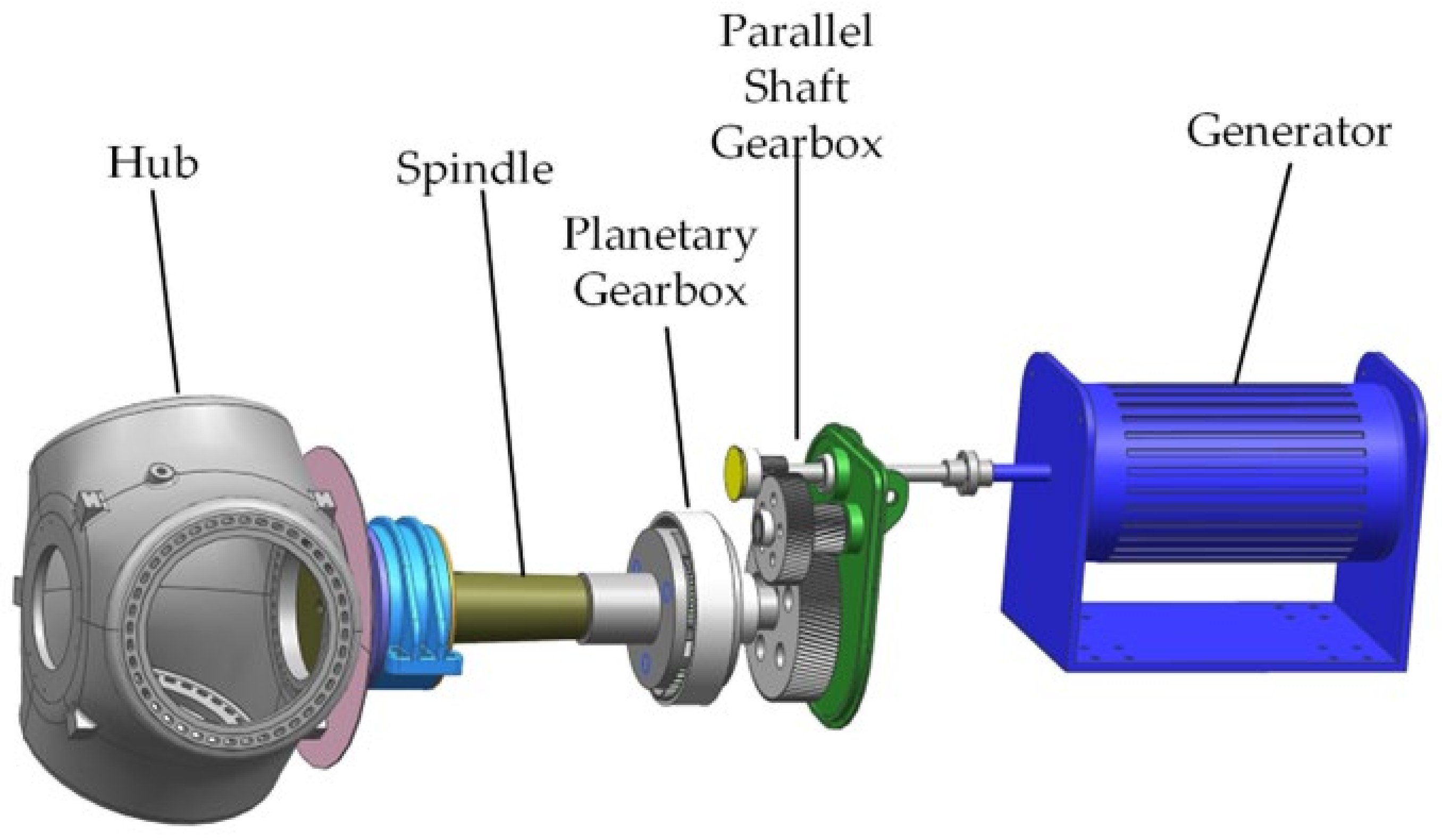
3.1. Lightweighting of Wind Turbine Drive Train Models

Due to the highly complex physical structure of wind turbine generators, accurately constructing models in virtual space would demand extremely high computer performance, consuming vast amounts of memory and GPU. This would result in computer lag and delays. Given that digital twins require low latency, it is crucial to implement lightweight processing on the models.

Generally speaking, the lightweight processing of physical equipment models is divided into two steps. The first step involves the lightweight processing of the quantity of component features. Components that are invisible during the virtual module visualization process or have lower weight during operation are deleted or hidden, with only the primary parts such as the rotor hub, main drive shaft, planetary gearbox, parallel shaft gearbox, and generator retained after lightweight processing. The second step is the lightweight processing of the mesh features of the parts. Classic methods for lightweight mesh features include vertex clustering, region merging, and geometric deletion.

The edge-collapse algorithm within the geometric deletion method is a mainstream mesh lightweight algorithm, as illustrated in Figure 3. However, this method can lead to model deformation and feature loss when simplifying the original model. Consequently, Michael Garland et al. [16,17] proposed the Quadric Error Metrics (QEM) algorithm to improve the edge-collapse algorithm. It aims to minimize model deformation and feature loss as much as possible, enabling the rapid generation of high-quality simplified models.

The Quadric Error Metrics (QEM) algorithm defines the error before and after lightweight processing as the sum of squared distances from a vertex to the original adjacent edges. It then calculates the quadric error matrix for each vertex to obtain the edge-collapse weights, prioritizing the collapse of edges with lower weights during the edge-collapse operation.

The specific calculation process for weights is as follows: assume a plane in three-dimensional space is represented by $Ax+By+Cz+D=0$, where $A^2+B^2+C^2=1$, $D$ are constants; given any point $v={(m,n,o)}^T$ in space, the squared distance from $V$ to the plane is as follows:

$$d^2=\frac{{(Am+Bn+Co+D)}^2}{(A^2+B^2+C^2)}={(Am+Bn+Co+D)}^2$$

(2)

And $n=(A,B,C)$ is a unit normal vector to the plane, then the equation of the plane in space can also be represented as

$$n^T\cdot v+d=0$$

(3)

The Equations (2) and (3) implies the following:

$$d^2={(n^T\cdot v)}^2={(v^T\cdot n)}^2$$

(4)

Since the quadratic error at each vertex in the grid is defined as the sum of the squares of the distances to the adjacent faces, namely:

$$\begin{array}{cc}\hfill {\Delta }_v& ={{\displaystyle \sum _{n\in \alpha (v)}(v^T\cdot n)}}^2\hfill \\ \hfill & ={\displaystyle \sum _{n\in \alpha (v)}(v^T\cdot n)}(n^T\cdot v)\hfill \\ \hfill & ={\displaystyle \sum _{n\in \alpha (v)}{v}^T(n{n}^2)}v\hfill \\ \hfill & =v^T\left({\displaystyle \sum _{n\in \alpha (v)}{K}_n}\right)v\hfill \end{array}$$

(5)

$\alpha (v)$ represents the geometry of the adjacent triangles of the vertex, and T denotes any triangle plane in the set.

Let $Q_v$ be the quadratic error matrix for point $v$. Since the quadratic error matrix is a 4 × 4 matrix, denoted as $v={(m,n,o,1)}^T$, $n=(A,B,C,D)$, there is:

$$Q_v={\displaystyle \sum _{n\in \alpha (v)}{K}_n}$$

(6)

$$\begin{array}{cc}\hfill K_n& =n{n}^T\hfill \\ \hfill & \hfill =\left[\begin{array}{cccc}{A}^2& AB& AC& AD\\ AB& B^2& BC& BD\\ AC& BC& C^2& CD\\ AD& BD& CD& D^2\end{array}\right]\end{array}$$

(7)

When mesh lightweight is performed, the quadratic error matrix for two neighboring vertices is $Q_{v1}$, $Q_{v2}$, then the weight of the edge to be folded is as follows:

$$Q_{\overline{v}}=Q_{v1}+Q_{v2}$$

(8)

Then, the error of the new vertex after folding is as follows:

$$\begin{array}{cc}\hfill {\Delta }_{\overline{v}}& ={\overline{v}}^T{Q}_{\overline{v}}\overline{v}\hfill \\ \hfill & ={\overline{v}}^T\left(Q_{v1}+Q_{v2}\right)\overline{v}\hfill \\ \hfill & ={\overline{v}}^T\left({\displaystyle \sum _{n\in \alpha (v_1)}n{n}^T}+{\displaystyle \sum _{n\in \alpha (v_2)}n{n}^T}\right)\overline{v}\hfill \\ \hfill & ={{\displaystyle \sum _{n\in \alpha (v_1)}\left(n^T\cdot \overline{v}\right)}}^2+{{\displaystyle \sum _{n\in \alpha (v_2)}\left(n^T\cdot \overline{v}\right)}}^2\hfill \end{array}$$

(9)

According to Equation (9), the error measure of an edge is determined by the sum of the quadratic error matrices between the new vertex $\overline{v}$ and the two vertices on the same edge. Therefore, the sequence of edge folding is relevant to the overall mesh simplification of the model. When determining the new vertex, it is necessary to compute the point with the minimum error. Taking the partial derivative of Equation (9),

$$\frac{\partial {\Delta }_{\overline{v}}^{\prime }}{\partial x}=\frac{\partial {\Delta }_{\overline{v}}^{\prime }}{\partial y}=\frac{\partial {\Delta }_{\overline{v}}^{\prime }}{\partial z}=0$$

(10)

Then,

$$\left[\begin{array}{cccc}{q}_{11}& q_{12}& q_{13}& q_{14}\\ q_{21}& q_{22}& q_{23}& q_{24}\\ q_{31}& q_{32}& q_{33}& q_{34}\\ 0& 0& 0& 1\end{array}\right]\overline{v}=\left[\begin{array}{c}0\\ 0\\ 0\\ 1\end{array}\right]$$

(11)

$$\overline{v}={\left[\begin{array}{cccc}{q}_{11}& q_{12}& q_{13}& q_{14}\\ q_{21}& q_{22}& q_{23}& q_{24}\\ q_{31}& q_{32}& q_{33}& q_{34}\\ 0& 0& 0& 1\end{array}\right]}^{-1}\left[\begin{array}{c}0\\ 0\\ 0\\ 1\end{array}\right]$$

(12)

The position of the new vertex can be obtained according to the above. If Equation (11) is not invertible, the following hair method should be used to select the new vertex:

$$n\left(\overline{v}\right)=\left\{\begin{array}{c}{v}_1,\\ v_2,\\ \left(v_1+v_1\right)/2,\end{array}\begin{array}{c}{Q}_{v1}<Q_{v1}\\ Q_{v1}>Q_{v1}\\ Q_{v1}=Q_{v1}\end{array}\right.$$

(13)

After iterative algorithm operation, the model’s mesh is updated to obtain a lightweight model to ensure the optimal lightweight effect. The main components of the model after lightweighting are shown in Figure 4. The model is later saved in FBX format for use in building digital twins in Unity3D.

3.2. Construction of Kinematic Models for Transmission Systems

The kinematic model of the wind turbine is the key to accurately mapping its motion state, and the digital twin model incorporating the kinematic model can accurately map the actual wind turbine operation in virtual space in real-time, driven by real-time operation data. Therefore, in this paper, the kinematic modeling of the wind turbine drive train is carried out. Construct a dynamic model based on the working principles of the central transmission system and related essential components of the wind turbine generator, as shown in Figure 5.

Where ${\omega }_b$ is the hub speed; ${\omega }_c$ is the carrier speed; ${\omega }_p$ is the planetary gear speed; ${\omega }_s$ is the sun gear speed; ${\omega }_{g1}{\omega }_{g2}{\omega }_{g3}{\omega }_{g4}$ are the speeds of gears 1, 2, 3, and 4, respectively. $Z_s$, $Z_r$, $Z_p$, $Z_{g1}$, $Z_{g2}$, $Z_{g3}$, $Z_{g4}$, are the numbers of teeth on the sun gear, planet gear, ring gear, gear 1, gear 2, gear 3, and gear 4, respectively.

Let $\omega =({\omega }_b,{\omega }_c,{\omega }_s,{\omega }_{g1},{\omega }_{g2},{\omega }_{g3},{\omega }_{g4},{\omega }_g)$, and let $\eta$ be the matrix representing the speed relationships between each component, then:

$$\eta =\left[\begin{array}{cccccccc}1& 0& 0& 0& 0& 0& 0& 0\\ 0& 1& 0& 0& 0& 0& 0& 0\\ 0& 0& 1+\frac{Z_r}{Z_s}& 0& 0& 0& 0& 0\\ 0& 0& 0& 1& 0& 0& 0& 0\\ 0& 0& 0& 0& \frac{Z_{g2}}{Z_{g1}}& 0& 0& 0\\ 0& 0& 0& 0& 0& 1& 0& 0\\ 0& 0& 0& 0& 0& 0& \frac{Z_{g3}}{Z_{g4}}& 0\\ 0& 0& 0& 0& 0& 0& 0& 1\end{array}\right]$$

(14)

$${\omega }^T=\eta ·{\omega }^T=\left[\begin{array}{cccccccc}1& 0& 0& 0& 0& 0& 0& 0\\ 0& 1& 0& 0& 0& 0& 0& 0\\ 0& 0& \frac{Z_r}{Z_s}& 0& 0& 0& 0& 0\\ 0& 0& 0& 1& 0& 0& 0& 0\\ 0& 0& 0& 0& \frac{Z_{g2}}{Z_{g1}}& 0& 0& 0\\ 0& 0& 0& 0& 0& 1& 0& 0\\ 0& 0& 0& 0& 0& 0& \frac{Z_{g3}}{Z_{g4}}& 0\\ 0& 0& 0& 0& 0& 0& 0& 1\end{array}\right]\left[\begin{array}{l}{\omega }_b\\ {\omega }_c\\ {\omega }_s\\ {\omega }_{g1}\\ {\omega }_{g2}\\ {\omega }_{g3}\\ {\omega }_{g4}\\ {\omega }_g\end{array}\right]=\left[\begin{array}{l}{\omega }_b\\ {\omega }_b\\ {\omega }_b\left(1+\frac{Z_r}{Z_s}\right)\\ {\omega }_b\left(1+\frac{Z_r}{Z_s}\right)\\ {\omega }_b\left(1+\frac{Z_r}{Z_s}\right)\cdot \frac{Z_{g2}}{Z_{g1}}\\ {\omega }_b\left(1+\frac{Z_r}{Z_s}\right)\cdot \frac{Z_{g2}}{Z_{g1}}\\ {\omega }_b\left(1+\frac{Z_r}{Z_s}\right)\cdot \frac{Z_{g2}}{Z_{g1}}\cdot \frac{Z_{g3}}{Z_{g4}}\\ {\omega }_b\left(1+\frac{Z_r}{Z_s}\right)\cdot \frac{Z_{g2}}{Z_{g1}}\cdot \frac{Z_{g3}}{Z_{g4}}\end{array}\right]$$

(15)

According to Figure 5, the dynamic equation between the hub and the low-speed shaft is as follows:

$$T_b=J_b{\ddot{\theta }}_b+C_1({\dot{\theta }}_c-{\dot{\theta }}_b)+K_1({\theta }_c-{\theta }_b)$$

(16)

$$T_c=C_1({\dot{\theta }}_c-{\dot{\theta }}_b)+K_1({\theta }_c-{\theta }_b)$$

(17)

In Equations (16) and (17), $J_b$ and ${\theta }_b$ represent the rotational inertia and angular displacement of the hub, respectively; $T_c$, $C_1$, $K_1$, and ${\theta }_c$ represent the torque, damping, stiffness, and angular displacement of the low-speed shaft, respectively. For the gearbox, in order to simplify mathematical modeling, it is treated as a whole, with the low-speed shaft as the input shaft and the high-speed shaft as the output shaft. Therefore, its dynamic equation is:

$$T_c+\eta \cdot T_{g4}=0$$

(18)

In Equation (18), $\eta$ represents the gear ratio of the gearbox; thus,

$$\eta =\left(1+\frac{Z_r}{Z_s}\right)\cdot \frac{Z_{g2}}{Z_{g1}}\cdot \frac{Z_{g3}}{Z_{g4}}$$

(19)

Therefore, the dynamic equation between the high-speed shaft and the generator is as follows:

$$T_{g4}=J_g{\ddot{\theta }}_g+C_2({\dot{\theta }}_g-{\dot{\theta }}_{g4})+K_2({\theta }_g-{\theta }_{g4})$$

(20)

$$T_g=T_{g4}-C_2({\dot{\theta }}_g-{\dot{\theta }}_{g4})-K_2({\theta }_g-{\theta }_{g4})=J_g{\ddot{\theta }}_g$$

(21)

In Equations (20) and (21), $J_g$, ${\theta }_g$, and $T_g$ represent the rotational inertia, angular displacement, and torque of the generator, respectively; $T_{g4}$, $C_2$, $K_2$, and ${\theta }_{g4}$ represent the torque, damping, stiffness, and angular displacement of the high-speed shaft, respectively.

3.3. Digital Twin Model Building and Driving

Models are imported into the virtual scene and assembled based on positional data, and then the operating forms of the components in the scene are scripted using a programming language so that they can be driven according to actual movement conditions. In this way, natural operating conditions are reproduced. The hierarchical relationship and operation logic between the components in the virtual module are shown in Figure 6. The hierarchy determines its motion logic, and the higher levels determine the absolute position of the lower levels.

In order to realize the real-time mapping of the virtual model, the physical module and the virtual module are connected to drive the twin model according to the real-time data collected in real-time. When it is necessary to check the historical operation condition, the twin model can be driven by the historical data composed of the real-time data stored in the daily work, and the historical operation process can be reproduced.

4. Fault Diagnosis Method Based on Digital Twin

4.1. Implementation Method of Fault Diagnosis System Based on Digital Twin

The benefits of digital twin technology in troubleshooting lie in its ability to enable real-time monitoring, simulation, and emulation of natural systems, reduction in maintenance costs, optimization of repair solutions, and knowledge management and iterative optimization. Through real-time monitoring, digital twin technology can capture changes in the operational status of the actual system and compare it with the virtual model to detect potential signs of failure. In terms of simulation and emulation, digital twin technology can simulate the operation of the actual system in a virtual environment to quickly test different failure assumptions and repair options, reducing the cost and time of trial and error. Reducing maintenance costs is another significant advantage of digital twin technology. By analyzing equipment operation data, predictive maintenance can be achieved to identify and solve potential failures in a timely manner, avoiding production stoppages and increased maintenance costs brought about by sudden failures. Additionally, digital twin technology can achieve the accumulation and management of knowledge through the continuous analysis of maintenance records and operation data, providing data support for the continuous optimization of the system, which improves production efficiency and equipment reliability. In summary, digital twin technology has multiple advantages in fault diagnosis, which can help enterprises reduce maintenance costs, improve productivity, and enhance equipment reliability.

This chapter proposes a wind turbine condition monitoring and fault diagnosis system based on digital twin technology. The system utilizes a variety of sensors and data acquisition devices to collect data related to the operating state of the wind turbine. Subsequently, the actual operating state of the wind turbine drive train is mapped onto the digital twin model through digital twin technology, which enables us to monitor the operating state of the wind turbine in real-time and detect potential faults in time. The framework of the intelligent monitoring and fault diagnosis system for wind turbine drive trains based on digital twins is shown in Figure 7.

The SCADA system was connected with the digital twin platform for data connection; when the system was running, real-time operation data of wind turbines in the SCADA system was obtained through TCP/IP connection protocols and displayed in Unity3D. Meanwhile, vibration data collected by each sensor was input into the fault diagnosis model. According to the diagnosis results, the virtual model is driven to simulate the behavior of the real physical wind turbine in the whole scene and realize the virtual and natural interaction. Specific steps are as follows:

• Step 1: The digital twin fault diagnosis system of the wind power transmission system collects the vibration signal of the wind turbine.
• Step 2: The data acquisition card is used to convert the analog signal collected by the acceleration sensor into a digital signal and transfer it to the PC.
• Step 3: The collected data are saved as a .CSV or .txt file by data acquisition software and exported to Unity3D.
• Step 4: The IVMD-PSO-LSSVM is packaged as a DLL file and integrated into the digital twin file.
• Step 5: The digital twin periodically or manually invokes vibration signals for fault diagnosis.
• Step 6: The digital twin model updates its running status according to the diagnosis results and is displayed in Unity3D.

In order to ensure the real-time nature of the data, a transmission method and communication protocol with fast transmission speed and high accuracy should be used, and the wind turbine operation status data can be displayed in real-time first and then stored in the database or both can be processed in parallel. In the main interface, environmental information such as temperature, wind speed, and turbine operating status information are displayed in line graphs. By clicking on the Fault Information UI button, a C# script can be triggered to retrieve historical fault information and maintenance records stored in the database. The historical data-driven model in the database can reproduce the historical state. The data transmission method is shown in Figure 8.

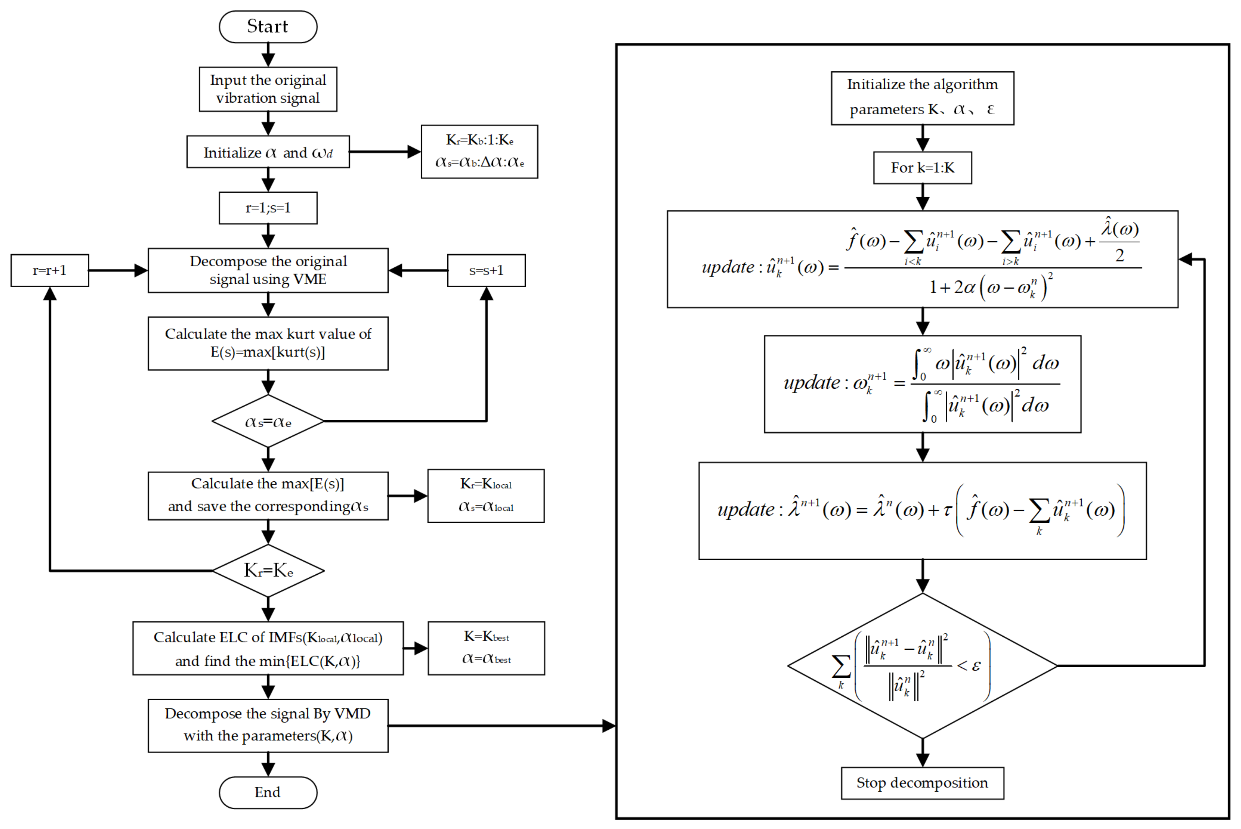
4.2. Feature Extraction Based on Improved Variational Modal Decomposition (IVMD)

Variational mode decomposition (VMD) [18,19] is an advanced technique for signal processing, particularly suitable for the analysis of nonlinear and non-stationary signals. It decomposes a complex real signal into several Intrinsic Mode Functions (IMFs) with certain central frequencies and finite bandwidths, achieving signal decomposition and reconstruction. These mode functions are independent of each other and have good sparsity, making VMD an effective tool for signal preprocessing and feature extraction.

When using the VMD algorithm to decompose a signal adaptively, the following input parameters are involved: modal decomposition parameter $K$, modal bandwidth control parameter $\alpha$, fidelity coefficient $\tau$, termination condition $\epsilon$. Among them, the modal decomposition parameter $K$ and the modal bandwidth control parameter α have a great influence on the decomposition effect of the VMD algorithm. The modal decomposition parameter $K$ determines the number of IMF components after the decomposition of the VMD algorithm; when the $K$ value is set too large, it produces problems such as modal aliasing and false components, while when the $K$ value is set too small, it leads to the phenomenon of under-decomposition, and the complex signals are not effectively separated, which causes certain troubles to the subsequent signal processing. The modal bandwidth control parameter α mainly affects the frequency bandwidth of each IMF component and the convergence speed in the decomposition process. When α is set too large, the frequency bandwidth of each IMF component becomes narrowed, resulting in signal loss. In addition, a value of $\alpha$ that is too large also leads to large fluctuations in the center frequency of the IMF components during the decomposition process, long decomposition time, and low signal-to-noise ratio of the decomposed components, which affects the decomposition effect and accuracy of the VMD algorithm. When the value of α is set too small, although the shock components in the signals can be detected more efficiently, at the same, there are more noise components and modal overlapping problems. Therefore, choosing the appropriate decomposition parameters $K$ and $\alpha$ becomes a major problem for the VMD algorithm in signal preprocessing applications.

To address this problem, Zhang Fan et al. [20] proposed a method for adaptively selecting the decomposition parameters ($K$, $\alpha$) of the VMD algorithm. This method adaptively determines $K$ and $\alpha$ by combining the kurtosis index with the energy loss coefficient. The flowchart is shown in Figure 9.

The kurtosis index reflects the impulse characteristics of the signal and is sensitive to early weak faults. A series of locally optimal parameter pairs are preliminarily selected based on the maximum kurtosis criterion. The formula for calculating kurtosis is as follows:

$$e(i)=\frac{1}{N}{{\displaystyle \sum _{i=1}^N\left(\frac{u_i-\overline{u}}{\sigma }\right)}}^4$$

(22)

Herein, $u_i$ represents the modal component IMFi, $N$ is the length of the pattern, $\overline{u}$ represents the average of $u_i$, and σ is the standard deviation of $u_i$.

In order to search for the optimal value of the VMD decomposition parameter $K_r$ within the range $[K_b,K_e]$, the step size is set to 1, ${\alpha }_s\in [{\alpha }_b,{\alpha }_e]$. The search step size is set to $\alpha$. Assuming the mode number for decomposition is $k$, and the bandwidth control parameter is ${\alpha }_s$, this pair of parameters is used to perform the VMD decomposition. After the decomposition, the kurtosis of each Instantaneous Mode Function (IMF) is calculated using Formula (3), and the highest value is deemed the kurtosis value for the current combination of parameters $(k,{\alpha }_s)$. Then, using the parameters $(k,{\alpha }_{s+\Delta \alpha })$, the signal is decomposed again by VMD, and the kurtosis values of each IMF are recalculated. The maximum kurtosis value is then taken as the kurtosis value for $(k,{\alpha }_{s+\Delta \alpha })$. This cycle continues until ${\alpha }_s={\alpha }_e$. The value of $\alpha$ corresponding to the maximum kurtosis value in the obtained sequence is taken as the optimal $\alpha$ for that mode number $k$. Subsequently, the mode number is set to $k+1$, and the cycle continues until $k=K_e$. Then, a series of locally optimal parameters can be obtained. The mathematical expression is represented as follows:

$$\begin{gathered} \overrightarrow{e_s^k}=\max (e_s^1,e_s^2,\dots ,e_s^k) \\ {e}_{lobal}^k=(e_b^k,e_{b+\Delta \alpha }^k,\cdots ,\overrightarrow{e_s^k},\cdots ,e_e^k) \\ {\alpha }_{lobal}^k=\arg \max (e_{lobal}^k) \end{gathered}$$

(23)

After obtaining a series of locally optimal parameter pairs, decompose the signal using the locally optimal parameter combinations. Then, the energy loss coefficient (ELC) of the modal components is calculated, and the parameters with the least energy loss are selected as the globally optimal VMD decomposition parameters. The formula for calculating ELC is as follows:

$$ELC=\frac{{‖f(t)-{\displaystyle \sum _{k=1}^K{u}_k}‖}_2^2}{\Vert f(t){\Vert }_2^2}$$

(24)

where $f(t)$ represents the signal, and $u_k$ is the modal component

The modal component signals obtained after preprocessing the vibration signals above retain the frequency characteristics of the original signals to the maximum extent and eliminate the noise and other irrelevant signals accordingly. In order to better realize fault state recognition, it is also necessary to carry out effective feature extraction on the preprocessed modal component signals. The purpose of feature extraction is to extract representative features from the original vibration signals and to use fewer low-dimensional feature vectors to represent a large amount of high-dimensional raw data.

Due to the complexity of vibration signals in the drive train, the original Normalized Dispersion Entropy (NDE) [21] cannot effectively describe the signal characteristics; hence, the Normalized Composite Multi-scale Dispersion Entropy (NCMDE) algorithm is introduced to describe signal features.

For a discrete sequence $x[n]$ of length $N$, it is first coarse-grained, as shown in Equation (25), to obtain its coarse-grained sequence under scale $\tau$, denoted as $\left\{x_1^{\tau },x_2^{\tau },\dots ,x_{\tau }^{\tau }\right\}$.

$$x_k^{\tau }[m]=\left\{{\displaystyle \sum _{i=\tau (m-1)+k}^{\tau m+k-1}x[i]}\right\}/\tau ,k\in [1,\tau ],m\in [1,N/\tau ]$$

(25)

The distribution probability of each scale in the coarse-grained sequence is calculated. The calculation steps are consistent with the original entropy calculation method. The distribution probability of the coarse-grained sequence under scale $\tau$ is obtained, denoted as $\left\{p_1^{\tau },p_2^{\tau },\dots ,p_{\tau }^{\tau }\right\}$. The mean distribution probability is calculated, and the NCMDE value is obtained, as shown in Equation (26).

$$\left\{\begin{array}{l}NCMDE(xt,c,m,d,\tau )=\frac{1}{\ln (c^m)}{\displaystyle \sum _{i=1}^{c^m}{\overline{p}}_{\tau }\left[{\pi }_i\right]\ln \left({\overline{p}}_r\left[{\pi }_i\right]\right)}\hfill \\ {\overline{p}}_r=mean(p_k^{\tau })\hfill \end{array}\right.$$

(26)

4.3. Particle Swarm Optimization Algorithm Optimizing Least Squares Support Vector Machine (PSO-LSSVM)

Support vector machine (SVM) [22] is a supervised learning algorithm widely used for classification and regression tasks. It is based on the principle of structural risk minimization in statistical learning, aiming to find an optimal decision boundary called the maximum margin hyperplane to maximize the margin distance between different classes. SVM deploys kernel techniques to handle nonlinear problems by mapping the data into a higher-dimensional space, making data that are nonlinearly separable in the original space linearly separable in the new space.

SVM, as a classical machine learning method, has been successful in many fields, but it also has some drawbacks. First, SVM has high computational complexity when dealing with large-scale datasets, especially for nonlinear kernel functions, which require a lot of computational resources and time. Second, SVM is more sensitive to parameter selection, including the selection of kernel function and the setting of regularization parameters, which need to be repeatedly tested and adjusted. In addition, when the number of positive and negative samples in the training dataset varies greatly, the classification performance of SVM may be affected, which is prone to the classification bias problem caused by sample imbalance.

In order to address some of the shortcomings of SVM, the least squares support vector machine (LSSVM) [23] proposes a series of improvements. First, LSSVM transforms the original problem into a convex quadratic optimization problem with constraints by introducing a regularization term, which reduces the computational complexity and is more efficient, especially when dealing with large-scale datasets. Secondly, LSSVM can automatically select the optimal parameters using methods such as cross-validation, which reduces the subjectivity of parameter adjustment and improves the generalization ability and stability of the model. In addition, LSSVM introduces more kinds of kernel functions, such as polynomial kernel function and radial basis function (RBF) kernel function, which makes the model more suitable for dealing with nonlinear problems and improves the classification performance. In summary, LSSVM improves computational efficiency, parameter selection, and nonlinear problem handling compared to traditional SVM, which makes the model more suitable for real-world scenarios and shows better performance in some specific application scenarios.

The core idea of LSSVM is that, for a set of training samples, $H=\{(x_i,y_i)|i=1,2,\dots ,n\}$, where $x_i\in R_n$ is the input data, and $y_i\in (-1,1)$ is the output data. When projecting sample data into a high-dimensional feature space, consider the nonlinear mapping $f(x_i)$ to construct the optimal decision function $y_i=({\omega }^{T}f(x_i)+\epsilon )$, where $\omega$ and $\epsilon$ are model parameters solved optimally as follows:

$$\left\{\begin{array}{c}{f}_{min}\left(\omega ,e_i\right)=\frac{1}{2}\Vert \omega {\Vert }^2+\frac{C}{2}{\displaystyle \sum _{i=1}^n}{e}_i^2\hfill \\ \mathrm{s}.\mathrm{t}.y_i=\left({\omega }^{T}f\left(x_i\right)+\epsilon \right)+e_i\hfill \end{array}\right.$$

(27)

In Equation (27), $\omega$ and $\epsilon$, respectively, represent the weight vector and bias; $e_i$ represents the error variable; $C$ represents the regularization parameter; $f(x)$ is the mapping function corresponding to the input data $x_i$.

The solution for $\omega$ and $\epsilon$ can be expressed as follows:

$$L\left(\omega ,\epsilon ,e_i,\lambda \right)=\frac{1}{2}{\omega }^2+\frac{C}{2}\underset{i=1}{\sum ^n}{e}_i^2-\underset{i=1}{\sum ^n}{\lambda }_i\left(\left({\omega }^{T}f\left(x_i\right)+\epsilon \right)+e_i-y_i\right)$$

(28)

Taking partial derivatives with respect to $\omega$, $\epsilon$, $e_i$, and $\lambda$ (where ${\lambda }_i\in R$ is a Lagrange multiplier), it can be expressed as follows:

$$\left[\begin{array}{cc}0& I\\ I^T& T+C^{-1}E\end{array}\right]\left[\begin{array}{c}\epsilon \\ \lambda \end{array}\right]=\left[\begin{array}{c}0\\ Y\end{array}\right]$$

(29)

In the Equation (29), $I=[1,1,\dots ,1]T$; $Y=[y_1,y_1,\dots ,y_1]T$; $\lambda =[{\lambda }_1,{\lambda }_2,\dots ,{\lambda }_n]$; $T=f(x_i)\cdot f(x_j)$; $Ei\times j$ is the identity matrix; $K(x_i,x_j)=(f(x_i),f(x_j))$ is the kernel function. At this point, given a training sample set $H=\{(x_i,y_j)|i=1,2,\dots ,n\}$, the equation can be solved to obtain $\lambda$ and $\epsilon$, resulting in a decision function, which can be expressed as:

$$f(x)=\mathrm{sgn}\left[{\displaystyle \sum _{i=1}^n{\lambda }_{i}K(x_i,x_j)}+\epsilon \right]$$

(30)

Particle swarm optimization (PSO) [24] is a swarm intelligence algorithm characterized by its simplicity and fast convergence speed. Its core idea is first to define a certain number of free particles and then use an automatic iterative process to calculate the optimal solution of the objective function. Each particle represents a possible solution, and intelligent problem-solving is achieved through the simple behavior of particles and the interaction of group information. In each iteration process, in order to find parameter values that meet the given requirements, it is necessary to track the changes in two “extremes” and continuously adjust the positions of particles. When the value of a particle reaches the optimal solution of its iteration process, it is called the individual extreme value ($pBest$), and the individual extreme value is shared with random particles in the entire population. Another extreme value is the optimal solution obtained by the entire population, called the global extreme value ($gBest$). The optimal solution found by the particle itself means that only some of the population has found the optimal solution. After finding $pBest$ and $gBest$ through iteration, each random particle’s position and velocity are updated according to Equation (31).

$$V=wV+c_{1}rand()(pBest-p)+c_{2}rand()(gBest-p)$$

(31)

$$p=p+V$$

(32)

In this context, $rand()$ is a random function value between (0,1); $c_1$ and $c_2$ are known as learning factors; $w$ is referred to as the weighting factor; $V$ is known as the velocity of the particle’s movement; $p$ is referred to as the particle’s current position.

As the iteration process continues, the value of $w$ changes according to the trend of a monotonically decreasing function, causing $w_{\max }$ to transition further to $w_{\min }$.

$$w=w_{\max }-iter\times (w_{\max }-w_{\min })/ite{r}_{\max }$$

(33)

Here, “$iter$” refers to the current number of iterations in PSO, and “$ite{r}_{\max }$” refers to the maximum number of iterations in PSO.

This paper uses the training accuracy during the training process as the objective function for particle swarm optimization least squares support vector machine (PSO-LSSVM). The final optimization problem can be transformed into finding the optimal parameters $({\sigma }^2,C)$. Through iterative calculation, the maximum value of the objective function is finally obtained. The specific implementation process of PSO-LSSVM is shown in Figure 10.

4.4. Fault Diagnosis Model

Based on the theory outlined in the previous section, we designed a hybrid IVMD-PSO-LSSVM method for diagnosing faults within the wind turbine drive train. Taking gearbox bearings as an example, the program flow of the method is shown in Figure 11 with the following steps:

• Step 1: The vibration signals of wind turbine bearings are collected under different fault conditions.
• Step 2: The kurtosis index and the energy loss coefficient are used to determine the optimal parameter pairs ($K_{best}$, ${\alpha }_{best}$) of the VMD, and then the raw vibration signal is decomposed into several IMF components.
• Step 3: Based on the minimum envelope entropy criterion, the optimal IMF component is selected for subsequent analysis.
• Step 4: Feature vectors containing rich fault information from optimal IMF components are extracted using the NCMDE algorithm.
• Step 5: The optimal combination of penalty factor c and kernel function parameters are determined for LSSVM using the PSO algorithm.
• Step 6: The extracted feature vector is randomly divided into training and test samples. The training samples are used to train the LSSVM after optimizing the parameters, and the test samples are used to test the trained LSSVM, which ultimately verifies the effectiveness and superiority of the method proposed in this paper.

Suppose one wants to apply the above-proposed fault diagnosis model to an already-built wind turbine model. This requires connecting MATLAB and Unity3D; this problem is a call to the DLL file generated by MATLAB. The communication between MATLAB software and Unity3D software is achieved by calling the MATLAB program in C# language. First, the MATLAB program is compiled into a DLL program, then the DLL call is made using the C# language, and finally, by clicking on the fault diagnosis UI button, a C# script can be triggered to use the functions in the DLL program.

5. Case Study

5.1. Experimental Verification of Fault Diagnosis Model

In order to verify the effectiveness of the above diagnostic algorithm, we need to perform adequate experiments to prove it. However, conducting fault diagnosis experiments directly on actual wind turbines faces many challenges, such as high costs and safety risks, and there needs to be more real fault data for wind turbines. To overcome these difficulties, our lab purchased the Wind Turbine Drivetrain Diagnostics Simulator (SQi-WTDS) as a platform for testing the effectiveness of the wind turbine transmission fault diagnosis algorithm, as shown in Figure 12.

The SQi-WTDS test platform is a high-fidelity alternative model featuring a two-stage parallel axis gearbox and a planetary gearbox. The parallel axis gearbox has straight-cut gears with a module of 1.5 and transmission ratios of 39:90 and 29:100. The bearing models and parameters are shown in

Table 2. Bearing parameters used for the experiment.

Bearing Type	Number of Scrollers	Rolling Body Diameter	Pitch Circle Diameter
ER-16K	9	7.9375	38.5064

. This test bench shares the same transmission structure as real wind turbine gearboxes, ensuring that the platform can accurately simulate the operational status and fault characteristics of wind turbine drive trains under various operating conditions. However, achieving such consistency is extremely difficult in real wind turbines due to the variability of operating conditions and environmental factors. Therefore, we selected the SQi-WTDS test platform solely to validate the accuracy of the proposed IVMD-PSO-LSSVM fault diagnosis model.

We conducted a set of rolling bearing experiments in the gearbox to verify the performance of the algorithm, and we collected the bearing vibration data under normal, inner ring fault, outer ring fault, and rolling body fault conditions, respectively. The parameters and solid photos of the bearings used for the experiment are shown in Table 2 and Figure 13.

In this experiment, the rolling bearing vibration data were collected using a CT1005LC acceleration sensor with a charge sensitivity of 49.7 mV/g. The acceleration sensor was placed directly under the right bearing end cap of the input shaft of the spur gearbox, as shown in Figure 14. Experiments were conducted to collect vibration data from the rolling bearings under different loads and different rotational speeds, as shown in

Table 3. Vibration data collection conditions.

Bearing Condition	Load (A)	Rotate Speed	Class Label
Normal	1.2/1.5	1200/1500	1
Inner ring fault	1.2/1.5	1200/1500	2
Outer ring fault	1.2/1.5	1200/1500	3
Rolling body fault	1.2/1.5	1200/1500	4

(there are four working conditions, namely 1.2 A/1200 rpm, 1.2 A/1500 rpm, 1.5 A/1200 rpm, and 1.5 A/1500 rpm).

During data acquisition, the sampling frequency was set to 20,480 Hz, and the sampling time was 2 s. Under each working condition, 20 groups of rolling bearing vibration data were collected under normal, inner ring failure, outer ring failure, and rolling element failure, with 2048 data points in each group, totaling 320 groups.

Figure 15 shows the time domain waveforms of the vibration signals of rolling bearings in various states under 1.2 A load and 1200 rpm rotation speed. It can be seen that the waveforms of the vibration signals in different states are different in the time domain, but it is not easy to summarize and analyze their laws directly, so it is necessary to process the vibration signals accordingly.

To validate the feasibility and superiority of the proposed IVMD algorithm, this section decomposes the experimental data using both the conventional VMD algorithm and the IVMD algorithm and compares the decomposition results. Taking the outer ring fault vibration signal in Figure 15 as an example, based on a previous experience [25], the mode decomposition parameter K in VMD is set to 4, and the mode bandwidth control parameter α is set to 2000. The decomposition results are shown in Figure 16a. It can be seen that the original signal is decomposed into four IMF components, each with an independent characteristic frequency, and the frequency bands between the components are distinctly separated. This indicates that each component obtained through the VMD algorithm can effectively retain the frequency characteristics of the original signal and effectively eliminate invalid components. However, there is evident over-decomposition in IMF2 and IMF3, and the central frequencies of IMF3 and IMF4 are too large, indicating possible under-decomposition. Next, we use IVMD to decompose this set of signals. The search range and step size of $K$ and $\alpha$ are preliminarily set as $K\in \left[2,7\right]$ and $\alpha \in \left[1000,\mathrm{10,000}\right]$, respectively, and the search step size $\Delta \alpha =500$. Select the best VMD parameters according to the above IVMD algorithm flow. By calculating the minimum ELC value, the optimal decomposition parameters for IVMD (5, 2000) were determined. Using (5, 2000) as the IVMD decomposition parameters, the signal is decomposed, and the results are shown in Figure 16b. It can be seen that the components obtained through the IVMD algorithm do not exhibit cross-phenomena, demonstrating that the IVMD algorithm can effectively mitigate the mode mixing problem. The central frequencies of the IMF components are closely spaced without under-decomposition, proving that the modal components obtained through IVMD decomposition can comprehensively reflect the frequency characteristics of the original signal and effectively eliminate false components and noise.

To further validate the effectiveness of the IVMD algorithm, we selected the IMF3 component from VMD and the IMF4 component from IVMD based on the minimum envelope entropy criterion for envelope analysis. The results are shown in Figure 17. From Figure 17a, it can be seen that the envelope spectrum of the signal decomposed by IVMD clearly shows the fault characteristic frequency and harmonics. In contrast, Figure 17b shows that the fault characteristic frequency in the signal decomposed by VMD contains many interferences, hindering the extraction of fault characteristics. In summary, the proposed IVMD algorithm can effectively decompose signals.

The optimal IMF component of the rolling bearing under each working condition is obtained from the above section, and then the NCMDE algorithm is used to extract the feature of each IMF component to construct the feature vector set for the following fault mode recognition.

In order to test the performance of the classification model, we use four different fault diagnosis models to conduct the fault classification experiment, namely, IVMD-LSSVM, VMD-PSO-LSSVM, IVMD-PSO-SVM, and IVMD-PSO-LSSVM. According to the previous experience [20], in each state, 29 sets of data are extracted at a ratio of 1:1 as the training set for the subsequent fault recognition model and 29 sets of data as the test set for the model, so there are 116 training sets and 116 test sets in the experimental rolling bearing vibration dataset. We input the mentioned data into these models for training and testing. First, the signal is decomposed by IVMD, let the search range and step size of $K$ and $\alpha$ be $K\in \left[2,7\right]$ and $\alpha \in \left[1000,\mathrm{10,000}\right]$, respectively, and the search step size $\Delta \alpha =500$; the tolerance error (tol) is set to $1\times {10}^{-7}$, and the maximum number of iterations is set to 50. The signal is then decomposed using IVMD, and according to the minimum envelope entropy criterion, the optimal IMF components are selected. After that, feature extraction is performed on the IMF components, setting the NCMDE parameters, where the class $c$, embedding dimension $m$, and delay $d$ are set to 6, 3, and 1, respectively. The NCMDE features are calculated in the scale range of 4–9 and combined with 10 time-domain features, including mean, variance, root mean square, absolute mean amplitude, skewness, kurtosis, crest factor, waveform factor, pulse factor, and margin factor, as well as 3 frequency-domain features, including center frequency, mean square frequency, and frequency variance, resulting in a total of 19-dimensional data to construct the feature vector set, which is then input into PSO-LSSVM for fault mode identification. For this experiment, the PSO algorithm is set with a population size of 200, a maximum of 50 iterations, learning factors $C_1$ and $C_2$ both set to 2, the width ${\sigma }^2$ of the Gaussian kernel function set in the range of $\left[0.01\sim 200\right]$, and the penalty coefficient $C$ set in the range of $\left[0.01\sim 300\right]$. The experimental results are shown in detail in Figure 18 and

Table 4. Diagnostic accuracy and computation time for four different combinations of algorithmic models.

Signal Decomposition Algorithm	Classification Algorithm	Accuracy	Time
VMD	PSO-LSSVM	95.7%	14.4 s
IVMD	LSSVM	96.6%	16.8 s
IVMD	PSO-SVM	98.3%	26.4 s
IVMD	PSO-LSSVM	99.1%	21.2 s

.

The above experimental results show that compared with other diagnostic models, the IVMD-PSO-LSSVM algorithm has excellent performance, the diagnostic results are extremely accurate, and it can accurately detect and identify various types of faults. At the same time, under the premise of ensuring accuracy, its computational efficiency is outstanding, and large-scale data processing and analysis can be completed in a very short period of time, providing a reliable guarantee for fast and efficient fault diagnosis.

5.2. Implementation of Fault Diagnosis System of Wind Turbine Transmission System Based on Digital Twin

In this paper, a wind farm with a 750 KW fan is taken as an example. The digital twin-based wind turbine drive train fault diagnosis system proposed above is tested for normal and rolling body failures. The sensor selection includes through-frequency acceleration sensors, and their performance indicators are presented in

Table 5. Through-frequency acceleration sensor parameters.

Sensor Type	Sensitivity	Measuring Range	Frequency Range	Operating Temperature
RH103	100 mV/g	80 g	0.5~15,000 Hz (±3 dB)	−40~120 °C

; the position of each sensor is shown in Figure 19. Data acquisition is performed using a microprocessor-based intelligent data acquisition system, which comprises several distributed boards and other components. Eventually, various sensors’ outputs are converted into signals that can be accepted by the A/D converter.

The digital twin fault diagnosis system established in this paper is shown in Figure 20, which is divided into four modules: the main interface, the status monitoring module, the digital twin model module, the fault diagnosis module, and the alarm recording module. The left side of the main interface shows the basic information about the wind turbine, and the middle screen shows the digital twin model monitor, in which the monitoring position is the wind turbine drive train, and the monitor can be free to slide the viewpoint through the monitor to observe the operation status of the wind turbine directly. The bottom right is the real-time vibration information when the wind turbine is running in the time-domain diagram, and the bottom left is the history of the running information.

The condition monitoring module is capable of responding to collected data presented in both the time domain graph and the frequency domain graph. This study encompasses a total of six data monitoring channels, each corresponding to one of the six sensors integrated into the system. Users can freely switch between the data from any of these sensors, allowing for comprehensive monitoring and analysis. Each sensor provides real-time data that can be visualized in the time domain graph, which shows how the sensor readings change over time, and the frequency domain graph, which displays the distribution of the sensor signal frequencies. This dual-domain analysis enables a more detailed understanding of the equipment’s operational status and potential anomalies. The interface is shown in Figure 21. By taking sensor 2 example, the interface reads the collected data and performs a Fourier transform on the data to display the time domain diagram of the data.

The digital twin modeling module is used to respond to the actual operating conditions of the physical equipment. The model is driven by a built-in kinematic model that can simulate the actual operation of the physical equipment based on information such as wind speed, spindle speed, blade angle and fault type. During the operation of the equipment, the digital twin model can collect and process various sensor data in real time, so as to accurately reproduce the operation status of the physical equipment. When a fault is encountered, the model can directly locate the screen to the fault location and can freely slide the viewpoint to observe the condition of each wind turbine component, helping staff to quickly find the fault and analyze the cause. The digital twin model not only reflects the operational status of the equipment in real time, but also detects possible faults and issues timely alerts, thus improving the maintenance efficiency and operational reliability of the equipment. In addition, the model’s user interface is designed to be intuitive and easy to operate, making it possible for non-technical personnel to master it quickly. It can show the internal structure and operation of the equipment through three-dimensional visualization, enabling maintenance personnel to more intuitively understand the operating status and fault conditions of the equipment. Through comparative analysis of historical data, the model can also provide trends and causes of failures, helping to optimize equipment operation strategies and maintenance plans. Figure 22 shows a model view of a wind turbine drive system during normal operation, while Figure 23 demonstrates the fault angle localization function using a medium-speed bearing rolling element failure as an example. By showing the operation of the faulty component in detail, this function allows maintenance personnel to determine the root cause of the problem faster, saving time for troubleshooting and repair, and improving the operational efficiency and reliability of the wind turbine.

The fault diagnosis module is a functional module used to call the IVMD-PSO-LSSVM algorithm model, the built-in algorithm every 20 min to call the algorithm for diagnosis of each sensor data, or manually in the status monitoring module to select the corresponding sensor click on the fault diagnosis button to call the data for diagnosis, and subsequently can be modified in the background IVMD-PSO-LSSVM to other fault diagnosis algorithm model.

The history module records information on historical fault diagnosis and equipment maintenance records.

During the wind turbine operation, if the algorithm is not practical in detecting new faults, the fault data can be saved and combined with a virtual simulation model to simulate the new fault state, and the resulting simulation data can assist in algorithm training and improve the algorithm’s robustness.

In order to verify the effectiveness of the digital twin model, we input the collected spindle speed data into the digital twin model and compare the collected high-speed shaft simulation data of the gearbox of the digital twin model with the actual measurement data. The results are shown in Figure 24. It can be seen from the figure that the output shaft speed simulated by the digital twin model is equal to the theoretical value, which is very close to the real acquisition value, indicating that the digital twin model of the wind turbine transmission system can effectively simulate the actual operating state of the wind turbine transmission system.

6. Discussion

This paper proposes a wind turbine drive train fault diagnosis system based on digital twins, focusing on the critical technology development and its application, with the help of digital twins’ powerful three-dimensional immersive visual expression, which improves the degree of visualization of traditional fault diagnosis, and then realizes the fast and accurate diagnosis and fault root cause analysis of wind turbine drive train system. In the paper, a fault diagnosis model based on IVMD-PSO-LSSVM is proposed and integrated into the digital twin system so that the system is characterized by fast computational efficiency, high accuracy, and fast response speed, which better reflects the real-time and accuracy of the digital twin compared with the traditional digital twin system.

7. Conclusions

In this paper, a wind turbine drive train fault diagnosis system based on digital twin technology is proposed to solve the problems of low intelligence and visualization of the wind turbine drive train fault diagnosis system. By constructing a digital twin model of the wind turbine, the intelligent monitoring of the wind turbine is realized, and the system is experimentally verified. On the basis of the above research, this paper summarizes the key technologies implemented in this system as follows:

(1)

The kinematics equations of the wind turbine drive system are integrated into the digital twin model of the wind turbine drive system so that the model can simulate the real running state of the wind turbine by using data such as speed.

(2)

An IVMD-PSO-LSSVM fault diagnosis method based on digital twin technology is proposed, which improves the calculation accuracy and efficiency and better embodies the real-time accuracy of fault diagnosis.

(3)

Unity3D, cloud server, and database were utilized to complete the construction of the digital twin scenario, which realized the fault diagnosis of the wind turbine drive train based on the digital twin, as well as the real-time mapping of the virtual module and the physical module and the reproduction of the operation status of a certain time period in the past.

Digital twin is a multi-disciplinary, multi-physical quantity, multi-scale, multi-probability simulation process involving a wide range of disciplines. Since our research is in a limited subject area, the relevant expertise is not comprehensive enough, so our research on digital twin technology is not comprehensive enough, and there are still many problems. The digital twin system developed in this study aims to verify the feasibility and effectiveness of the method proposed in this paper, and there is still a considerable gap with the actual digital twin. Subsequent research work can further optimize and upgrade the system. Power loss caused by friction and component efficiency should also be considered in the construction of the digital twin model. The subsequent research will focus on solving these problems to improve the accuracy and practicability of the system. Data processing should also explore how to effectively collect, store, and manage large amounts of real-time data, including sensor data, historical data, and environmental data.

References

1. Strielkowski, W.; Civín, L.; Tarkhanova, E. Renewable energy in the sustainable development of electrical power sector: A review. Energies 2021, 14, 8240. [Google Scholar] [CrossRef]
2. Peng, H.; Li, S.; Shangguan, L. Analysis of wind turbine equipment failure and intelligent operation and maintenance research. Sustainability 2023, 15, 8333. [Google Scholar] [CrossRef]
3. Grieves, M.; Vickers, J. Digital twin: Mitigating unpredictable, undesirable emergent behavior in complex systems. In Transdisciplinary Perspectives on Complex Systems: New Findings and Approaches; Springer: Berlin/Heidelberg, Germany, 2017; pp. 85–113. [Google Scholar]
4. Lei, H.; Fanli, Z.; Wei, W. Digital twin method and application practice of spacecraft system driven by mechanism data. Digit. Twin 2024, 4, 2. [Google Scholar] [CrossRef]
5. Yin, Y.; Zheng, P.; Li, C. A state-of-the-art survey on Augmented Reality-assisted Digital Twin for futuristic human-centric industry transformation. Robot. Comput.-Integr. Manuf. 2023, 81, 102515. [Google Scholar] [CrossRef]
6. Wang, B.; Zhou, H.; Li, X. Human Digital Twin in the context of Industry 5.0. Robot. Comput.-Integr. Manuf. 2024, 85, 102626. [Google Scholar] [CrossRef]
7. Tao, F.; Zhang, H.; Zhang, C. Advancements and challenges of digital twins in industry. Nat. Comput. Sci. 2024, 4, 169–177. [Google Scholar] [CrossRef] [PubMed]
8. Wang, Y.; Sun, W.; Liu, L. Fault Diagnosis of Wind Turbine Planetary Gear Based on a Digital Twin. Appl. Sci. 2023, 13, 4776. [Google Scholar] [CrossRef]
9. Yan, J.; Möhrlen, C.; Göçmen, T. Uncovering wind power forecasting uncertainty sources and their propagation through the whole modelling chain. Renew. Sustain. Energy Rev. 2022, 165, 112519. [Google Scholar] [CrossRef]
10. Stetco, A.; Dinmohammadi, F.; Zhao, X. Machine learning methods for wind turbine condition monitoring: A review. Renew. Energy 2019, 133, 620–635. [Google Scholar] [CrossRef]
11. Liu, Z.; Sun, W.; Chang, S. Corn Harvester Bearing fault diagnosis based on ABC-VMD and optimized EfficientNet. Entropy 2023, 25, 1273. [Google Scholar] [CrossRef]
12. Yu, G.; Wu, P.; Lv, Z. Few-shot fault diagnosis method of rotating machinery using novel MCGM based CNN. IEEE Trans. Ind. Inform. 2023, 19, 10944–10955. [Google Scholar] [CrossRef]
13. Wang, Z.; Nie, P.; Liu, J. Bearing fault diagnosis based on a multiple-constraint modal-invariant graph convolutional fusion network. High-Speed Railw. 2024, 2, 92–100. [Google Scholar] [CrossRef]
14. Daems, P.J.; Peeters, C.; Matthys, J. Fleet-wide analytics on field data targeting condition and lifetime aspects of wind turbine drivetrains. Forsch. Ingenieurwesen 2023, 87, 285–295. [Google Scholar] [CrossRef]
15. Tao, F.; Xiao, B.; Qi, Q. Digital twin modeling. J. Manuf. Syst. 2022, 64, 372–389. [Google Scholar] [CrossRef]
16. Garland, M.; Heckbert, P.S. Surface simplification using quadric error metrics. In Proceedings of the 24th Annual Conference on Computer Graphics and Interactive Techniques, Los Angeles, CA, USA, 3–8 August 1997; pp. 209–216. [Google Scholar]
17. Chang, H.; Dong, Y.; Zhang, D. Review of Three-Dimensional Model Simplification Algorithms Based on Quadric Error Metrics and Bibliometric Analysis by Knowledge Map. Mathematics 2023, 11, 4815. [Google Scholar] [CrossRef]
18. Dragomiretskiy, K.; Zosso, D. Variational mode decomposition. IEEE Trans. Signal Process. 2013, 62, 531–544. [Google Scholar] [CrossRef]
19. Jiang, X.; Wang, J.; Shen, C. An adaptive and efficient variational mode decomposition and its application for bearing fault diagnosis. Struct. Health Monit. 2021, 20, 2708–2725. [Google Scholar] [CrossRef]
20. Zhang, F.; Sun, W.; Wang, H. Fault diagnosis of a wind turbine gearbox based on improved variational mode algorithm and information entropy. Entropy 2021, 23, 794. [Google Scholar] [CrossRef]
21. Rostaghi, M.; Azami, H. Dispersion entropy: A measure for time-series analysis. IEEE Signal Process. Lett. 2016, 23, 610–614. [Google Scholar] [CrossRef]
22. Suthaharan, S.; Suthaharan, S. Support vector machine. In Machine Learning Models and Algorithms for Big Data Classification: Thinking with Examples for Effective Learning; Springer: Berlin/Heidelberg, Germany, 2016; pp. 207–235. [Google Scholar]
23. Suykens, J.A.K.; Vandewalle, J. Least squares support vector machine classifiers. Neural Process. Lett. 1999, 9, 293–300. [Google Scholar] [CrossRef]
24. Kennedy, J.; Eberhart, R. Particle swarm optimization. In Proceedings of the ICNN’95-International Conference on Neural Networks, Perth, WA, Australia, 27 November–1 December 1995; IEEE: Piscataway, NJ, USA, 1995; Volume 4, pp. 1942–1948. [Google Scholar]
25. Li, H.; Fan, B.; Jia, R.; Zhai, F.; Bai, L.; Luo, X. Research on multi-domain fault diagnosis of gearbox of wind turbine based on adaptive variational mode decomposition and extreme learning machine algorithms. Energies 2020, 13, 1375. [Google Scholar] [CrossRef]
Figure 1. Digital twin system framework for wind turbine drivetrains.
Applsci 14 05991 g001
Figure 2. Wind turbine drive train 3D model.
Applsci 14 05991 g002
Figure 3. Model lightweight schematic.
Applsci 14 05991 g003
Figure 4. Modeling of wind turbine drive train after lightweighting.
Applsci 14 05991 g004
Figure 5. Kinematic modeling of wind turbine drive train.
Applsci 14 05991 g005
Figure 6. Hierarchical relationship diagram of wind turbine drive train components.
Applsci 14 05991 g006
Figure 7. Framework of intelligent monitoring and fault diagnosis system for wind turbines based on digital twins.
Applsci 14 05991 g007
Figure 8. Data transmission method of fault diagnosis system based on digital twin.
Applsci 14 05991 g008
Figure 9. Improved variational modal decomposition flowchart.
Applsci 14 05991 g009
Figure 10. Flowchart of PSO optimized LSSVM algorithm.
Applsci 14 05991 g010
Figure 11. Flowchart of IVMD-PSO-LSSVM algorithm.
Applsci 14 05991 g011
Figure 12. Wind turbine power transmission fault diagnosis comprehensive experimental platform.
Applsci 14 05991 g012
Figure 13. Bearings for four different operating conditions.
Applsci 14 05991 g013
Figure 14. Sensor position in the gearbox.
Applsci 14 05991 g014
Figure 15. Time domain waveform of vibration signals in different states of rolling bearing.
Applsci 14 05991 g015
Figure 16. Decomposition of the result and the resulting frequency domain graph: (a) VMD decomposition result; (b) IVMD decomposition result.
Applsci 14 05991 g016
Figure 17. Envelope analysis results: (a) IVMD envelope analysis results; (b) VMD envelope analysis results.
Applsci 14 05991 g017
Figure 18. Diagnostic accuracy of four different combinations of algorithmic models.
Applsci 14 05991 g018aApplsci 14 05991 g018b
Figure 19. Location of sensors in wind turbines.
Applsci 14 05991 g019
Figure 20. Wind turbine transmission system fault diagnosis system main interface.
Applsci 14 05991 g020
Figure 21. Vibration monitoring interface of digital twin system of wind turbine drive system.
Applsci 14 05991 g021
Figure 22. Model window of digital twin system of drive system of wind power unit under normal condition.
Applsci 14 05991 g022
Figure 23. Model window of digital twin system of drive system of wind power unit under fault condition.
Applsci 14 05991 g023
Figure 24. (a) Measured wind turbine spindle speed. (b) Digital twin model output shaft speed and real measured output shaft speed.
Applsci 14 05991 g024