

Robust Fault-Tolerant Control of a Five-Phase Permanent Magnet Synchronous Motor under an Open-Circuit Fault

 ,
,  ,
,  , and
, and 
Abstract
1. Introduction
2. Dynamic Model of FPPMSM
2.1. Healthy Model
2.2. Faulty Model under Open Circuit of Phase “a”
3. Optimal References for the Currents
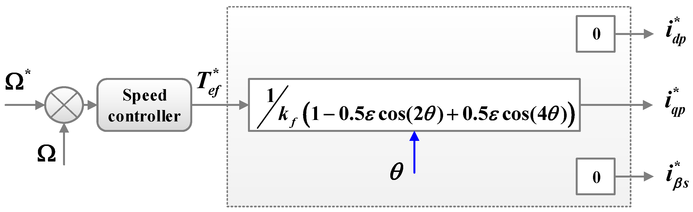
3.1. References in Healthy Conditions
3.2. References in Faulty Conditions
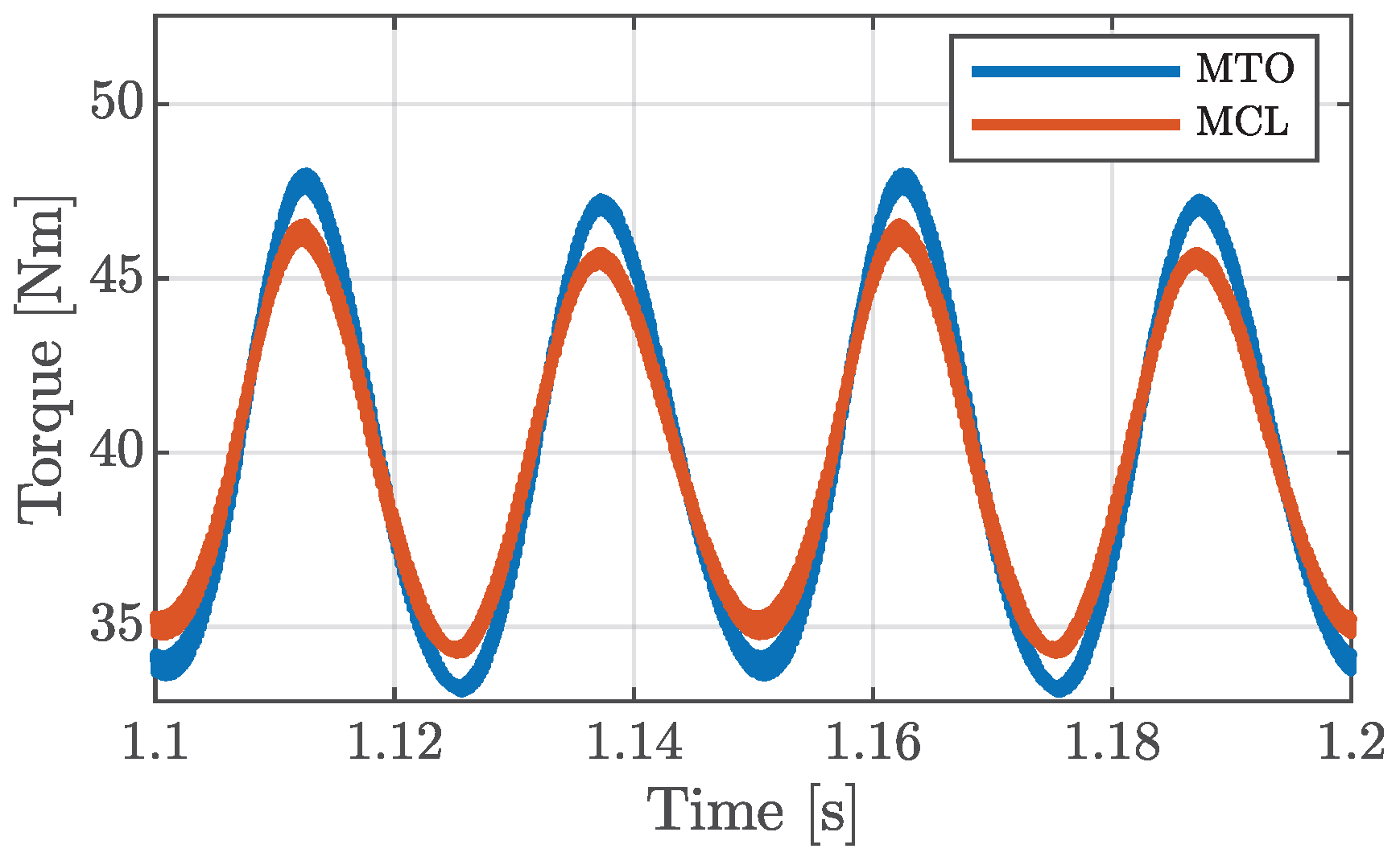
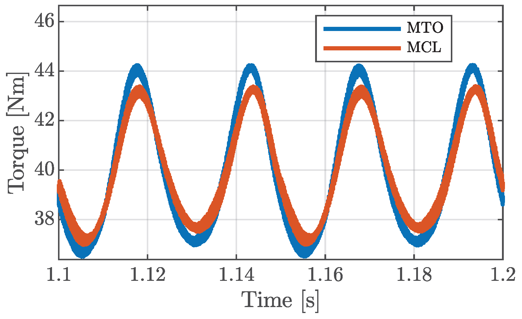
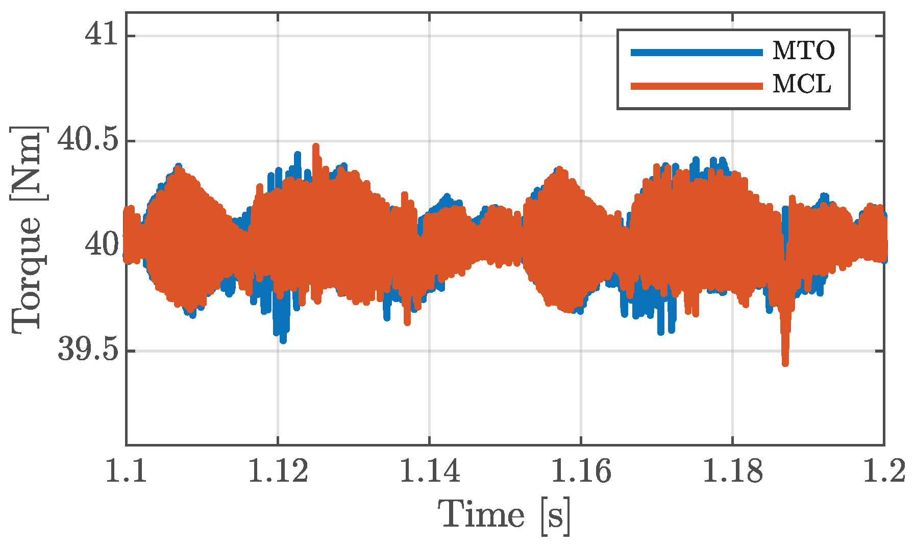
3.2.1. Criteria for the MCL Strategy
3.2.2. Criteria for the MTO Strategy
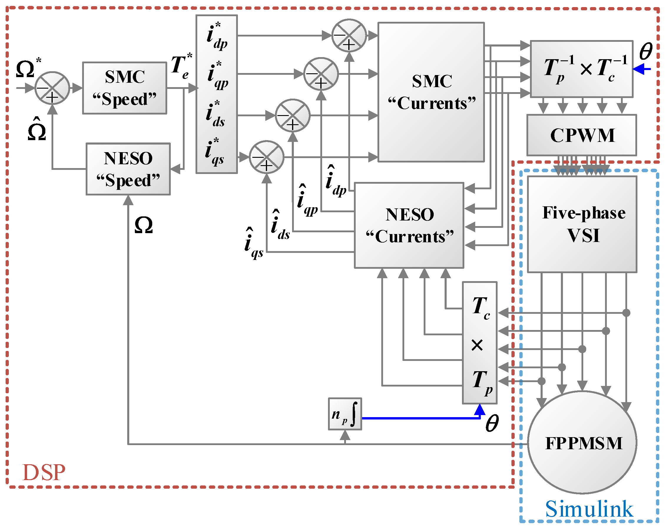
4. Design Combination of SMC and NESO
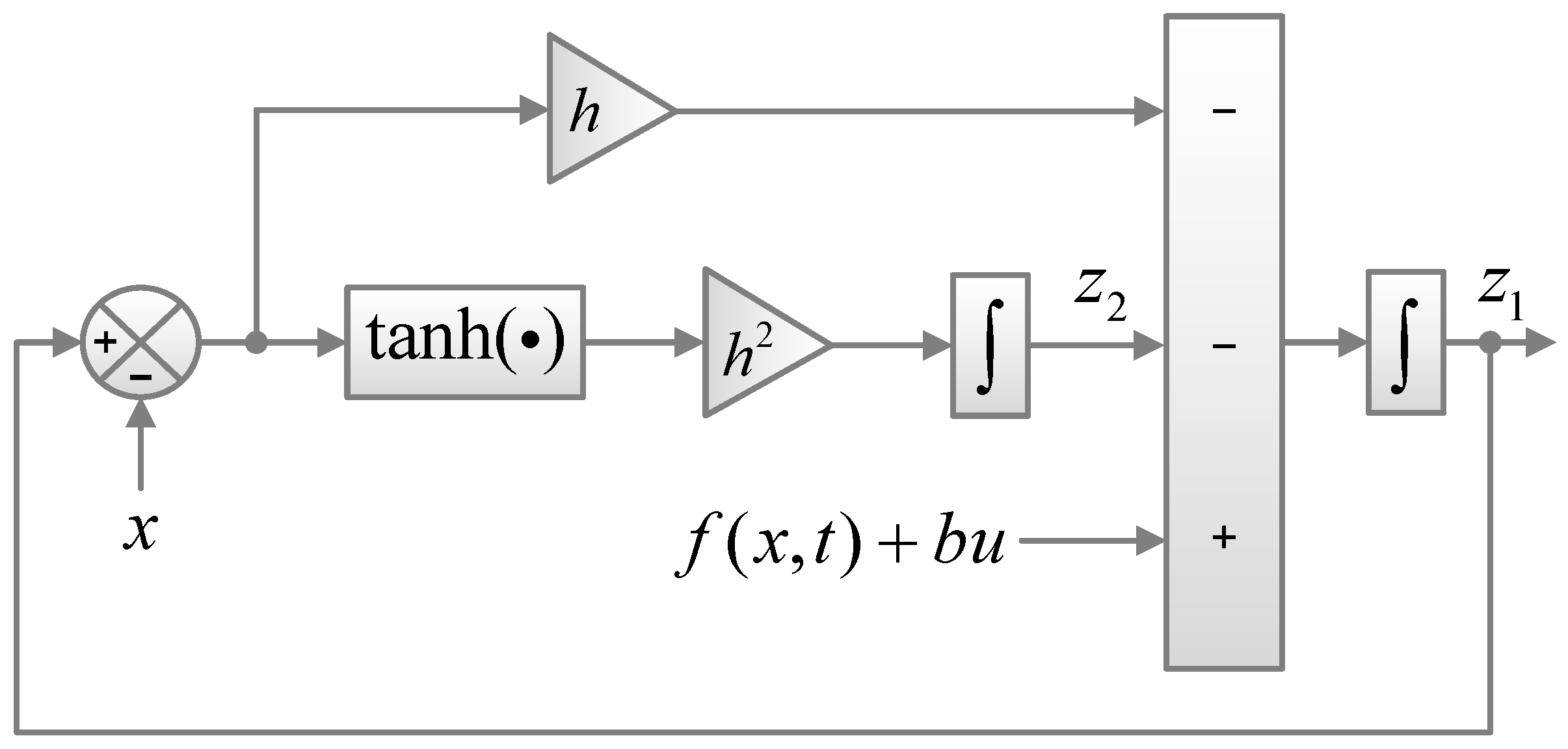
4.1. NESO Design
- Defining x, u, , and as , , , and , respectively, can be estimated by
- Defining x, u, , and as , , , and , respectively, can be estimated by
- Defining x, u, , and as , , , and , respectively, can be estimated by
- Defining x, u, , and as , , , and , respectively, can be estimated by
- Defining x, u, , and as , , , and , respectively, can be estimated by
- Defining x, u, , and as , , , and , respectively, can be estimated by
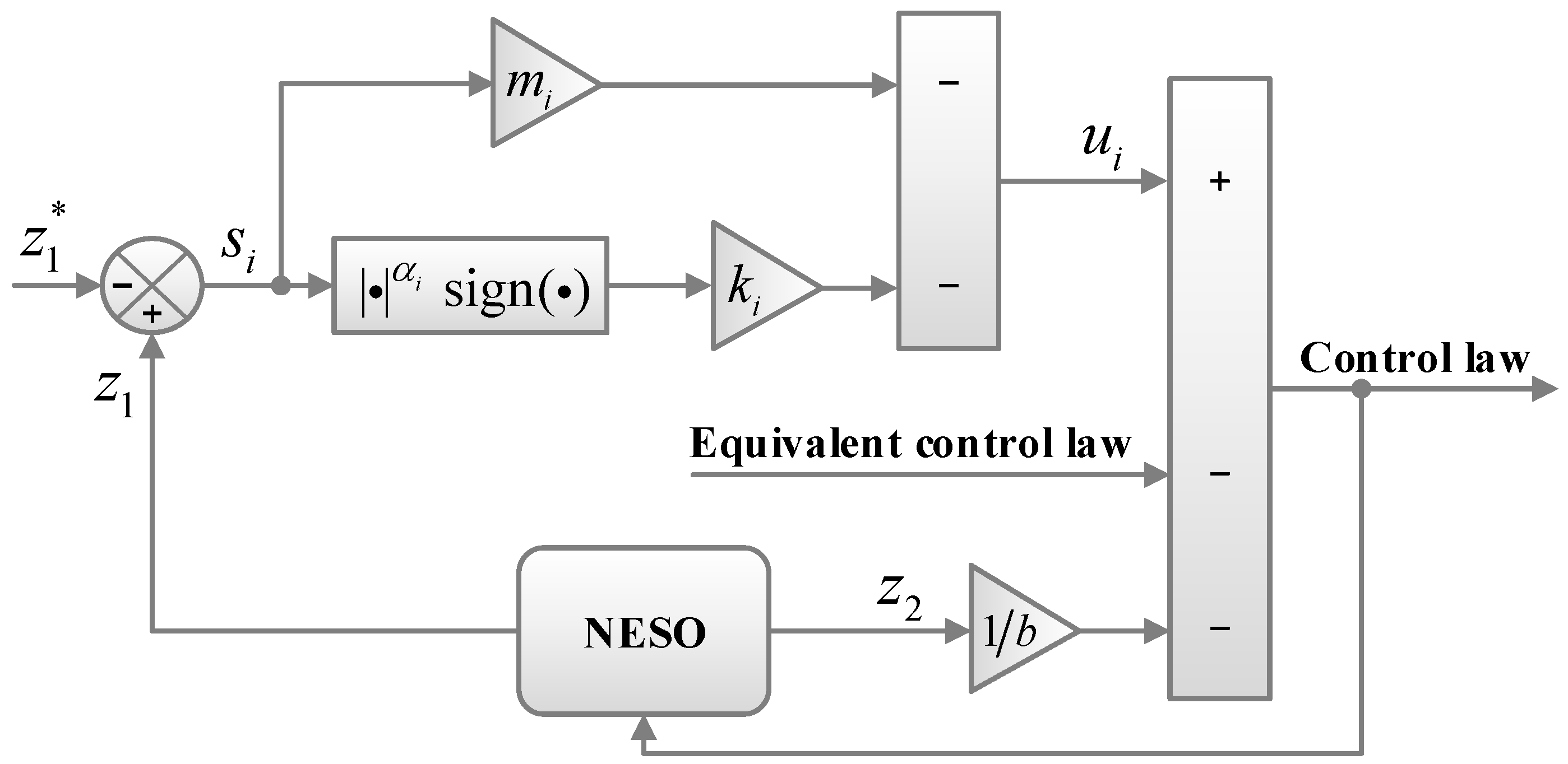
4.2. SMC Design
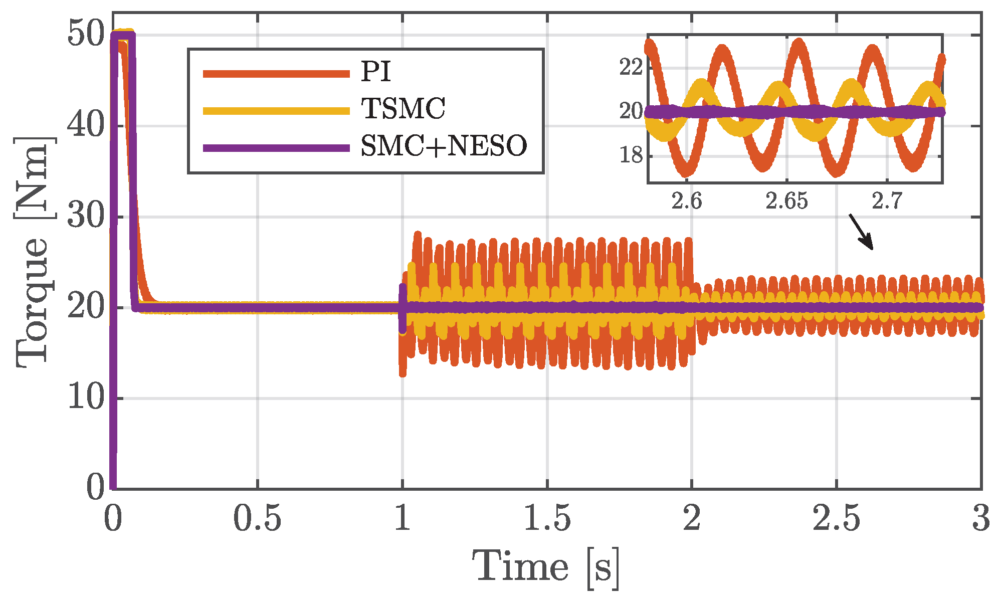
5. Results Analysis
5.1. Healthy Conditions
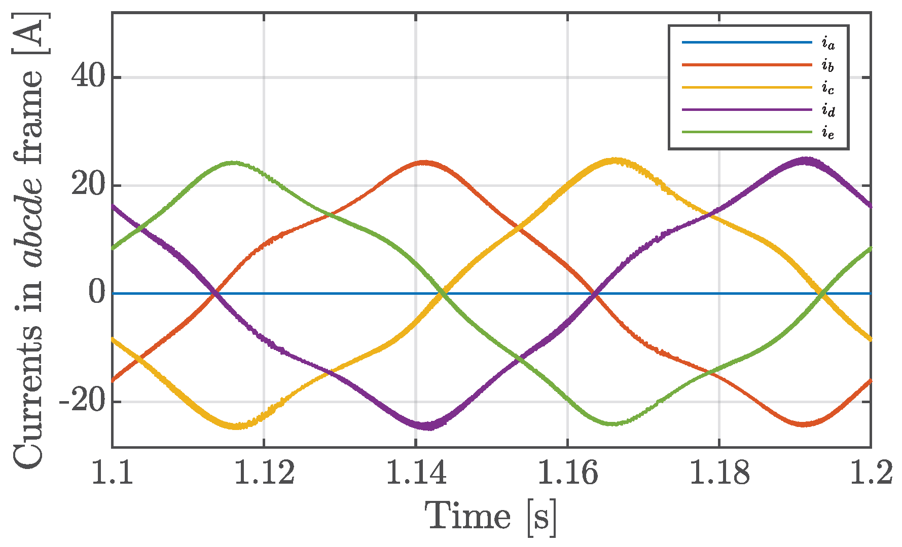
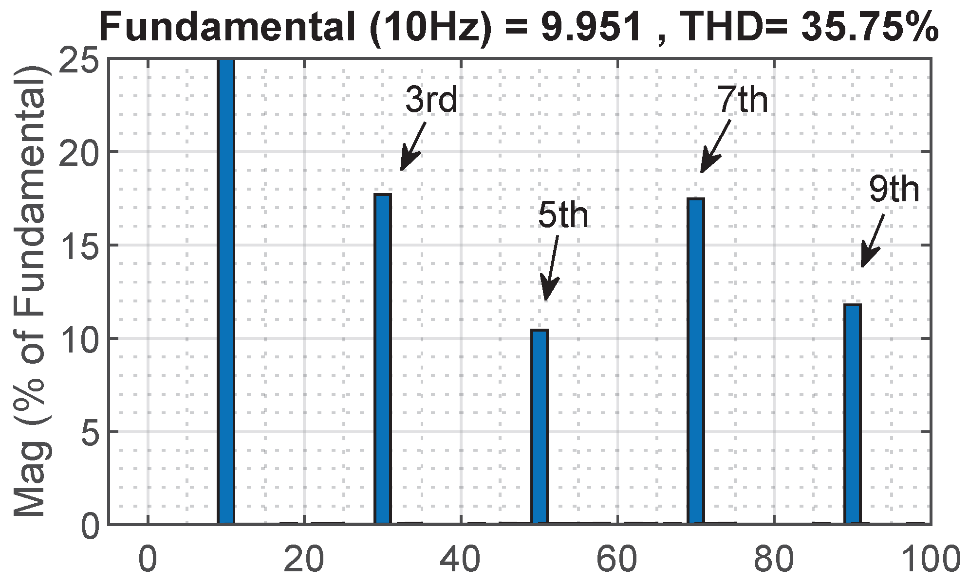
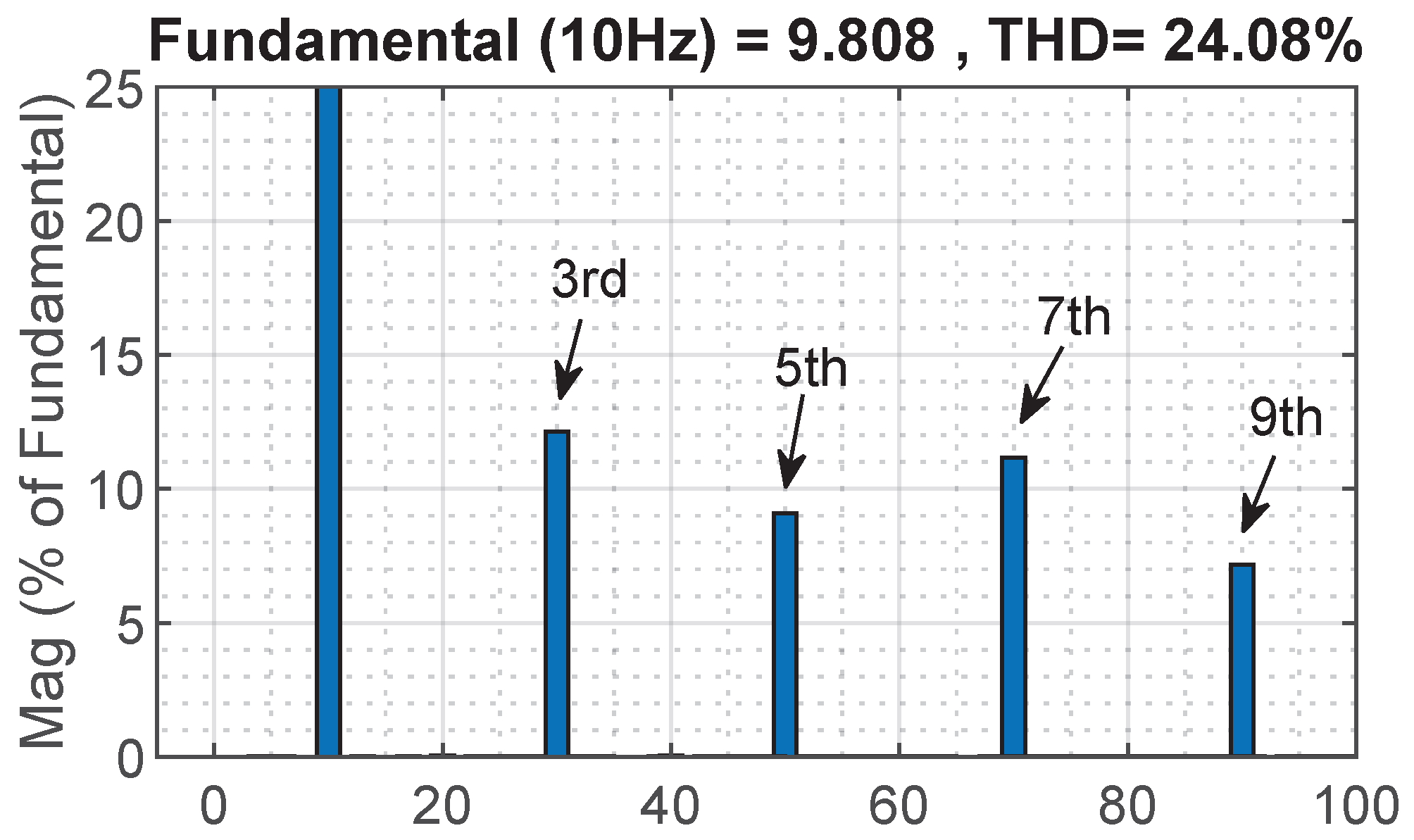
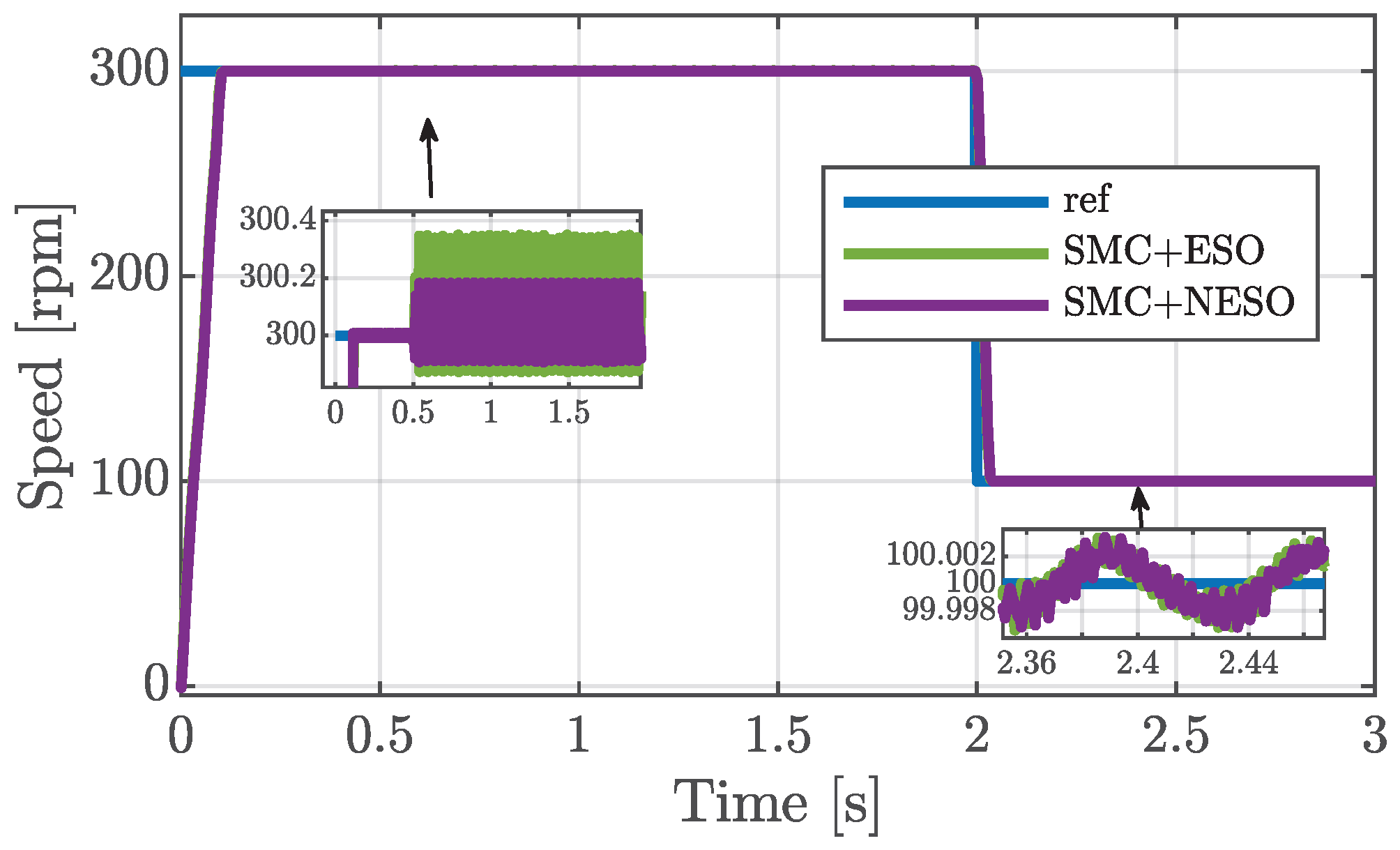
5.2. Faulty Conditions
6. Conclusions
Author Contributions
Funding
Institutional Review Board Statement
Informed Consent Statement
Data Availability Statement
Conflicts of Interest
Appendix A

| Parameter | Value |
|---|---|
| 2 | |
| 8.32 mH | |
| 6.54 mH | |
| 1.68 mH | |
| 1.78 mH | |
| 1.35 mH | |
| 0.512 Wb | |
| 0.034 Wb | |
| J | 0.095 kg·m2 |
| DC-link voltage | 150 V |
| Switching frequency | 10 kHz |
| Rated power | 3 kW |
| Rated speed | 1000 rpm |
| Maximum torque | 55 Nm |
| Peak phase voltage | 125 V |
| Peak phase current | 21 A |
References
- Zheng, Z.; Li, Q.; Li, X.; Zheng, P.; Wang, K.; Cui, P. Analysis and fault-tolerant control of inter-turn short-circuit fault for five-phase permanent-magnet synchronous machine. Energy Rep. 2022, 8, 7360–7373. [Google Scholar] [CrossRef]
- Oukrid, M.; Bernard, N.; Benkhoris, M.F.; Ziane, D. Design and Optimization of a Five-Phase Permanent Magnet Synchronous Machine Exploiting the Fundamental and Third Harmonic. Machines 2024, 12, 117. [Google Scholar] [CrossRef]
- Wei, Y.; Qiao, M.; Zhu, P. Fault-Tolerant Operation of Five-Phase Permanent Magnet Synchronous Motor with Independent Phase Driving Control. CES Trans. Electr. Mach. Syst. 2022, 6, 105–110. [Google Scholar] [CrossRef]
- Mo, S.; Ziane, D.; Oukrid, M.; Benkhoris, M.F.; Bernard, N. Dynamic Modeling Approach in View of Vector Control and Behavior Analysis of a Multi-Three-Phase Star Permanent Magnet Synchronous Motor Drive. Energies 2024, 17, 1567. [Google Scholar] [CrossRef]
- Wang, X.; Ren, S.; Xiao, D.; Meng, X.; Fang, G.; Wang, Z. Fault-Tolerant Control of Open-Circuit Faults in Standard PMSM Drives Considering Torque Ripple and Copper Loss. IEEE Trans. Transp. Electrif. 2023. Early Access. [Google Scholar] [CrossRef]
- Khlaief, A.; Boussak, M.; Gossa, M. Open phase faults detection in PMSM drives based on current signature analysis. In Proceedings of the XIX International Conference on Electrical Machines—ICEM 2010, Rome, Italy, 6–8 September 2010; pp. 1–6. [Google Scholar]
- Parsa, L.; Toliyat, H.A. Fault-Tolerant Interior-Permanent-Magnet Machines for Hybrid Electric Vehicle Applications. IEEE Trans. Veh. Technol. 2007, 56, 1546–1552. [Google Scholar] [CrossRef]
- Qiu-Liang, H.; Yong, C.; Li, X. Fault-Tolerant Control Strategy for Five-Phase PMSM With Third-Harmonic Current Injection. IEEE Access 2018, 6, 58501–58509. [Google Scholar] [CrossRef]
- Xiong, C.; Xu, H.; Guan, T.; Zhou, P. Fault-tolerant FOC for five-phase SPMSM with non-sinusoidal back EMF. IET Electr. Power Appl. 2019, 13, 1734–1742. [Google Scholar] [CrossRef]
- Tian, B.; Sun, L.; Molinas, M.; An, Q.T. Repetitive Control Based Phase Voltage Modulation Amendment for FOC-Based Five-Phase PMSMs under Single-Phase Open Fault. IEEE Trans. Ind. Electron. 2021, 68, 1949–1960. [Google Scholar] [CrossRef]
- Elmorshedy, M.F.; Selvam, S.; Mahajan, S.B.; Almakhles, D. Investigation of high-gain two-tier converter with PI and super-twisting sliding mode control. ISA Trans. 2023, 138, 628–638. [Google Scholar] [CrossRef]
- Tian, B.; An, Q.T.; Duan, J.D.; Sun, D.Y.; Sun, L.; Semenov, D. Decoupled Modeling and Nonlinear Speed Control for Five-Phase PM Motor Under Single-Phase Open Fault. IEEE Trans. Power Electron. 2017, 32, 5473–5486. [Google Scholar] [CrossRef]
- Tian, B.; Mirzaeva, G.; An, Q.T.; Sun, L.; Semenov, D. Fault-Tolerant Control of a Five-Phase Permanent Magnet Synchronous Motor for Industry Applications. IEEE Trans. Ind. Appl. 2018, 54, 3943–3952. [Google Scholar] [CrossRef]
- Mossa, M.A.; Echeikh, H. A novel fault tolerant control approach based on backstepping controller for a five phase induction motor drive: Experimental investigation. ISA Trans. 2021, 112, 373–385. [Google Scholar] [CrossRef] [PubMed]
- Haruna, A.; Mohamed, Z.; Efe, M.; Abdullahi, A. Switched step integral backstepping control for nonlinear motion systems with application to a laboratory helicopter. ISA Trans. 2023, 141, 470–481. [Google Scholar] [CrossRef] [PubMed]
- Labbadi, M.; Cherkaoui, M. Novel robust super twisting integral sliding mode controller for a quadrotor under external disturbances. Int. J. Dyn. Control 2020, 8, 805–815. [Google Scholar] [CrossRef]
- Wang, Y.; Feng, Y.; Zhang, X.; Liang, J. A New Reaching Law for Antidisturbance Sliding-Mode Control of PMSM Speed Regulation System. IEEE Trans. Power Electron. 2020, 35, 4117–4126. [Google Scholar] [CrossRef]
- Gao, W.; Hung, J. Variable structure control of nonlinear systems: A new approach. IEEE Trans. Ind. Electron. 1993, 40, 45–55. [Google Scholar]
- Wang, A.; Wei, S. Sliding Mode Control for Permanent Magnet Synchronous Motor Drive Based on an Improved Exponential Reaching Law. IEEE Access 2019, 7, 146866–146875. [Google Scholar] [CrossRef]
- Shi, S.L.; Li, J.X.; Fang, Y.M. Extended-State-Observer-Based Chattering Free Sliding Mode Control for Nonlinear Systems With Mismatched Disturbance. IEEE Access 2018, 6, 22952–22957. [Google Scholar] [CrossRef]
- Qu, S.; Xu, W.; Zhao, J.; Zhang, H. Design and Implementation of a Fast Sliding-Mode Speed Controller With Disturbance Compensation for SPMSM System. IEEE Trans. Transp. Electrif. 2021, 7, 2611–2622. [Google Scholar] [CrossRef]
- Liu, Z.; Houari, A.; Machmoum, M.; Benkhoris, M.F.; Tang, T. ESO-based FTC strategy via dual-loop compensations for 5-phase PMSG integrated tidal applications. IEICE Electron. Express 2021, 18, 20210177. [Google Scholar] [CrossRef]
- Zhou, H.; Xu, J.; Chen, C.; Tian, X.; Liu, G. Disturbance-Observer-Based Direct Torque Control of Five-Phase Permanent Magnet Motor under Open-Circuit and Short-Circuit Faults. IEEE Trans. Ind. Electron. 2021, 68, 11907–11917. [Google Scholar] [CrossRef]
- Zeghlache, A.; Mekki, H.; Djerioui, A.; Benkhoris, M.F. Active Fault-tolerant Control for Surface Permanent Magnet Synchronous Motor Under Demagnetization Fault. Period. Polytech. Electr. Eng. Comput. Sci. 2024, 68, 12–20. [Google Scholar] [CrossRef]
- Liu, G.; Geng, C.; Chen, Q. Sensorless Control for Five-Phase IPMSM Drives by Injecting HF Square-Wave Voltage Signal into Third Harmonic Space. IEEE Access 2020, 8, 69712–69721. [Google Scholar] [CrossRef]
- Liu, Z.; Houari, A.; Machmoum, M.; Benkhoris, M.F.; Tang, T. An Active FTC Strategy Using Generalized Proportional Integral Observers Applied to Five-Phase PMSG based Tidal Current Energy Conversion Systems. Energies 2020, 13, 6645. [Google Scholar] [CrossRef]
- Liu, Z.; Karimi, H.R.; Yu, J. Passivity-based robust sliding mode synthesis for uncertain delayed stochastic systems via state observer. Automatica 2020, 111, 108596. [Google Scholar] [CrossRef]
- Liu, Z.; Chen, X.; Yu, J. Adaptive Sliding Mode Security Control for Stochastic Markov Jump Cyber-Physical Nonlinear Systems Subject to Actuator Failures and Randomly Occurring Injection Attacks. IEEE Trans. Ind. Inform. 2023, 19, 3155–3165. [Google Scholar] [CrossRef]
- Dordevic, O.; Jones, M.; Levi, E. A Comparison of Carrier-Based and Space Vector PWM Techniques for Three-Level Five-Phase Voltage Source Inverters. IEEE Trans. Ind. Inform. 2013, 9, 609–619. [Google Scholar] [CrossRef]
- Yang, J.; Chen, W.H.; Li, S.; Guo, L.; Yan, Y. Disturbance/Uncertainty Estimation and Attenuation Techniques in PMSM Drives—A Survey. IEEE Trans. Ind. Electron. 2017, 64, 3273–3285. [Google Scholar] [CrossRef]
- Tian, B.; Wei, J.; Molinas, M.; Lu, R.; An, Q.; Zhou, B. Neutral Voltage Modeling and Its Remediation for Five-Phase PMSMs Under Single-Phase Short-Circuit Fault Tolerant Control. IEEE Trans. Transp. Electrif. 2022, 8, 4534–4548. [Google Scholar] [CrossRef]


| Controllers | Strategy | ||
|---|---|---|---|
| PI | MTO | ||
| MCL | |||
| TSMC | MTO | ||
| MCL | |||
| SMC+NESO | MTO | ||
| MCL |
Disclaimer/Publisher’s Note: The statements, opinions and data contained in all publications are solely those of the individual author(s) and contributor(s) and not of MDPI and/or the editor(s). MDPI and/or the editor(s) disclaim responsibility for any injury to people or property resulting from any ideas, methods, instructions or products referred to in the content. |
© 2024 by the authors. Licensee MDPI, Basel, Switzerland. This article is an open access article distributed under the terms and conditions of the Creative Commons Attribution (CC BY) license (https://creativecommons.org/licenses/by/4.0/).
Share and Cite
Zeghlache, A.; Mekki, H.; Benkhoris, M.F.; Djerioui, A.; Ziane, D.; Zeghlache, S. Robust Fault-Tolerant Control of a Five-Phase Permanent Magnet Synchronous Motor under an Open-Circuit Fault. Appl. Sci. 2024, 14, 5190. https://doi.org/10.3390/app14125190
Zeghlache A, Mekki H, Benkhoris MF, Djerioui A, Ziane D, Zeghlache S. Robust Fault-Tolerant Control of a Five-Phase Permanent Magnet Synchronous Motor under an Open-Circuit Fault. Applied Sciences. 2024; 14(12):5190. https://doi.org/10.3390/app14125190
Chicago/Turabian StyleZeghlache, Ayyoub, Hemza Mekki, Mohamed Fouad Benkhoris, Ali Djerioui, Djamel Ziane, and Samir Zeghlache. 2024. "Robust Fault-Tolerant Control of a Five-Phase Permanent Magnet Synchronous Motor under an Open-Circuit Fault" Applied Sciences 14, no. 12: 5190. https://doi.org/10.3390/app14125190
APA StyleZeghlache, A., Mekki, H., Benkhoris, M. F., Djerioui, A., Ziane, D., & Zeghlache, S. (2024). Robust Fault-Tolerant Control of a Five-Phase Permanent Magnet Synchronous Motor under an Open-Circuit Fault. Applied Sciences, 14(12), 5190. https://doi.org/10.3390/app14125190