Abstract
This paper presents a concept of a routing algorithm for a network of sensors monitoring the condition of machinery and equipment operating in areas at risk of methane and/or coal dust explosion. It was assumed that the proposed algorithm would find application in sensor networks monitoring, among other things, oil pressure in powered roof supports and the position of powered roof support elements. The results of a literature analysis were presented, which included the simulation of sensor network routing algorithms, including, among others, reactive algorithms, proactive algorithms and algorithms based on so-called swarm intelligence (SI). As a result of the analyses, several algorithms were selected and implemented in a prototype sensor network. The characteristics of each of these algorithms are described. The article includes a description of the commissioning work of the network, which consisted of between 3 and 30 nodes. An analysis of the collected measurement data obtained for each criterion of the performance evaluation of the routing algorithms is presented.
1. Introduction
Currently, IIoT (Industrial Internet of Things) technology is being used to monitor the state of technological processes [1]. This concept involves the use of networks of interconnected devices, sensors and systems that enable monitoring, data collection and optimisation of production, logistics and operational processes. IIoT is finding increasing application in the coal mining industry. Wireless sensor networks are being used to monitor the condition of underground machinery and equipment, environmental conditions, and the health of miners working in crude coal mining [2,3,4,5,6,7,8,9,10,11]. Research is being carried out and solutions are being developed for the application of wireless sensor networks for monitoring rock conditions, measuring roof deformation, and using wireless optoacoustic devices to create escape routes in mines.
Due to the complex structure of such networks, it is crucial to properly design the information transmission system to be reliable, flexible and safe. It is particularly important to ensure the reliability of sensor networks operating under methane and/or coal dust explosion hazards. To enable mobility and ease of deployment, sensor networks are typically equipped with wireless data transmission inter-feeds. In addition, these networks make use of advanced transmission algorithms [12,13,14], known as intelligent routing algorithms, to efficiently manage the flow of data over a wide area network infrastructure.
This paper presents the process of developing routing algorithms for a sensor network dedicated to monitoring the operating parameters of powered roof supports [15,16,17,18].
2. Characteristics of Sensory Network Design in Hazardous Areas
Sensors mounted on the powered roof support include inclinometers, oil pressure sensors in the hydraulic legs and a wall face distance measurement module [17,18]. It is necessary to develop a routing algorithm (to manage data transmission in a network of sensors operating on a powered roof support), regarding the entire sensor network design process.
The first element to be considered when designing a sensor network is the characteristics of the environment in which the network will operate. Deployment of nodes of the network as sensors on a powered roof support operating in a longwall complex requires radio visibility of the access point. Deployment of the sensors does not secure radio visibility of the access point by each sensor, so a mesh topology is suggested for the network (in this topology, one sensor can transmit data to its neighbour). The sensor closest to the access point collects data from the grid and transmits them by a flameproof computer to the surface.
The design of the sensors (grid nodes) installed on the longwall complex must comply with the requirements of the ATEX directive [19], in the area of group I, category M1 equipment with intrinsic safety protection ‘ia’. The requirements for the design of the equipment enclosure mainly concern the surface resistance and mechanical strength. The electrical systems must be protected with regard to limiting the radiated energy of the radio beam and the battery power supply in the hazardous area. The designed routing algorithm should ensure adaptation to the design of a specific sensory network. The following criteria were adopted in evaluation of the algorithm:
- Packet arrival time to destination—selecting the route for the data packet that will be the shortest path to the access point. By optimising according to this criterion, it will be possible to increase the sampling time of such a network without having to buffer the data. It is assumed that simple microcontrollers (with small internal memory capacity) are installed in the nodes, due to the need for low power consumption. However, it is necessary to increase the sampling rate due to the need to record phenomena such as sinkholes and collapses so that they can be predicted and thus counteracted later.
- Network throughput, data transmission speed—we also want the network to be able to transmit as much data as possible at any one time, using the maximum available throughput of the radio modules.
- Energy consumption—minimising energy consumption to compensate the energy losses by electrical protection devices that increase energy consumption (using additional resistance to reduce the current causes the battery energy to dissipate as heat); minimising energy consumption also affects the use of smaller-sized batteries, which again reduces the size of the enclosure, reducing the surface where static charge can build up.
- Packet deliver ratio—reliability of operation; confirmation that the measured data reaches the recipient and is not lost. The lack of data buffering, due to limited internal memory, forces the algorithm to be more reliable in delivering data to the destination—protocols do not have mechanisms for confirming transmission.
3. Simulation Analysis of Routing Algorithms
Both reactive and proactive algorithms are used in current sensor networks [20,21,22]. Proactive algorithms maintain an up-to-date routing table at each node in the network. When the network evolves or the topology changes, the nodes exchange information to update the routing table. Proactive algorithms are used when the network has a fixed or frequently changing topology. Reactive algorithms, on the other hand, do not maintain a fixed routing table, but search for a route to a destination only when necessary, for example, to forward data to another node. Reactive algorithms are more suitable for networks with low traffic or a changing topology, as they do not require constant routing table updates.
When analysing the literature on the simulation tests of routing algorithms in sensor networks, a deterioration in parameters of networks where both reactive and proactive algorithms were used was noted (Figure 1). Within the scope of this article, a few of the cases are selected and described.
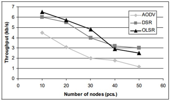
Figure 1.
Reactive and proactive algorithms [21].
In Figure 1, we can see that as the number of nodes increases, the network throughput decreases for the proactive AODV (ad hoc on-demand distance vector) algorithm, the proactive OLSR (optimised link state routing) algorithm and the reactive DSR (dynamic source routing) algorithm.
Figure 2 shows simulations of the reactive AODV (Figure 2a) and particle swarm optimisation (PSO)-based algorithms (Figure 2b). A network of 500 nodes was simulated. It can be clearly seen from the graphs that after the network stabilisation process, the PSO algorithm is able to maintain a higher and stable network throughput compared to the reactive algorithm.
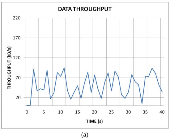
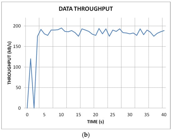
Figure 2.
AODV (a) and SSKIR (b) protocols [21].
Figure 3 shows the energy consumption of each node of proactive and reactive algorithms in relation to the beehive algorithm. Use of the Beehive algorithm minimises the energy consumption of the network node during data transmission (the energy required to transmit a certain amount of data through a node is the lowest for the beehive algorithm in comparison to reactive and proactive algorithms).
Figure 3.
Energy consumption—Beehive, DSR, AODV, DSDV algorithms [23].
The last simulation shown (Figure 4) is an analysis of the dependence of the routing algorithms on the packet delivery time to destination. The shortest packet delivery time was obtained for the network using the SICROA algorithm (based on the ACO ant algorithm). For the other algorithms, i.e., reactive AODV and proactive DSR, the packet delivery time was longer. In each case, the packet delivery time increased with the number of nodes in the network.
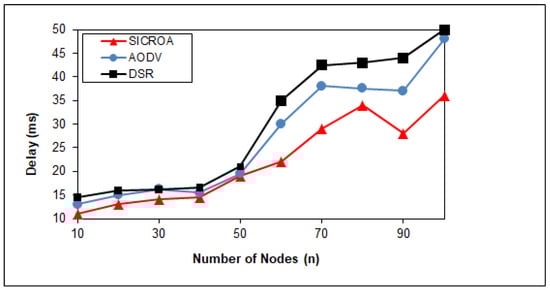
Figure 4.
Latency measurement with respect to node count [24].
Analysis of the network performance graphs as a function of the number of nodes shows that both proactive and reactive algorithms often experience performance degradation as the number of nodes increases. This is due to the increased network load, increased control traffic and data latency.
However, graph analysis of metaheuristics-based algorithms [25,26,27,28,29,30,31,32,33,34] such as particle swarm optimisation (PSO), ant colony optimisation (ACO) and bees algorithm (BEE) suggests that these algorithms have the ability to adapt communication routes more flexibly. The PSO algorithm, inspired by the behaviour of a swarm of birds or fish, can dynamically adjust communication routes in the network based on current conditions, while the ant colony algorithm (ACO), modelled on the way ants find the shortest routes, can find optimal communication routes between nodes even under changing conditions. In contrast, the bees algorithm (BEE), inspired by the foraging behaviour of bees, also has the ability to dynamically adjust communication routes in the network based on local information and interactions in the swarm. As a result, the BEE algorithm can efficiently find optimal communication routes in the sensory network, even under variable and dynamic environmental conditions.
To confirm the results of the simulation tests, it was decided to verify the performance of the algorithms in real hardware units. The following sections of the article discuss how the selected algorithms can be implemented in single hardware units.
4. Materials and Methods
Attempts were made to implement the selected algorithms based on swarm intelligence in hardware, such as the particle swarm optimisation algorithm [35,36,37,38], the ant swarm algorithm and the bee swarm algorithm. The modified particle swarm optimisation algorithm was successfully implemented in the sensor network model according to the assumptions. Each Pi-particle in the algorithm is defined by the b following relationship:
where:
—Dimension of the space in which the particle is located (in the case under consideration, it corresponds to the number of nodes in the network); the position of the particle in space is determined by the distance from all nodes of the network,
—i-th particle,
—position of the particle in D-dimensional space,
The algorithm calculates velocity and position using the following formula:
where:
—parameter that determines the weight of the previous position of the particle when determining the current position,
—k-th step of algorithm,
—i-th particle,
—scaling parameters,
—random numbers,
—best-fit local solution for i-th particle to the criterion,
—best-fit global solution to the criterion,
—time step length (it is assumed that the step length is equal to the unit time).
Initially, the values of the previous position and velocity, as well as the local and global criteria of the best-fit solution are randomly determined from the range (0, 1>. Each particle is a representation of a solution, where, in the context of this case, the solution is the path from a node of type NODE to a node of type SINK.
A specially designed objective function is used to find the optimal solution according to the following set of criteria :
where:
—weights for each criterion taking values in the range (0, 1>,
—power of the radio signal transmitted from a neighbouring node,
—battery charge level of the neighbouring node,
—number of hops, transmissions between NODE nodes on the way to a SINK node.
The objective function for determining the best local solution and the best global solution:
Once the criteria for the best fit are established, the position and velocity of each particle are recalculated. The computational process is carried out by the SINK node, based on the information received from the NODE nodes, collected during the execution of successive iterations. NODE nodes collect information about the state of their neighbours to then send to the SINK node.
In the context of the fixed table of neighbours of the NODE-type nodes of the:
where:
—parameters defining the neighbours of the node ,
The index for selecting the best neighbour is determined by the equation:
where:
— node location,
—number of available neighbours of the node .
The next step is to send information about the best neighbours to the NODE nodes behind the SINK node.
A modified version of the ACO (ant colony optimisation) algorithm [39,40,41] has been integrated with the sensor network model, with the following assumptions.
NODE nodes collect data about their neighbours (sent in FOLLOW_ME type packets). The data packets sent by NODE nodes, called ants, travel to neighbouring nodes selected on the basis of a probability function, leaving a pheromone in the visited nodes (which actually corresponds to the incrementation of a variable). The probability that an ant from node i will select node j is given by the following formula:
where:
—amount of pheromone left between node i and node j,
—local criterion function value for the transition from node i to node j,
—the set of nodes available to node i,
—coefficients determining the weight between the criterion function and the pheromone.
The local criterion function value is determined according to the following equation:
where:
—indicator of the strength of the radio signal received from a neighbouring node,
—the number of nodes through which the message travelled on its way to the SINK node,
—the battery charge level of the neighbouring node,
—the weights attributed to each criterion.
The probability function depends on the transmitter power of the neighbouring node, expressed as the RSSI parameter value, the number of hops to the SINK node and the battery level of the neighbouring node. In the context of this algorithm, the objective is to find routes from the NODE node to the SINK node that minimise the travel time. Nodes with a higher battery charge are also preferred as potential neighbours.
When an agent packet or ant reaches a SINK node, its route is compared with the routes of other agents. Out of all solutions, the optimum one is selected. After a certain number of iterations (number of agents sent), the SINK node sends information about the selected optimal path to all NODE nodes.
Information about the pre-selected neighbours is stored in the nodes. Based on this, the message (ant) repeats the path selection process on its way to the SINK node. The SINK node sends information confirming that the data packet has reached its destination. This process is repeated for a certain number of iterations, and is also performed when certain events occur, such as the loss of a node or the appearance of a new node in the network.
The modified bee algorithm [42,43] uses three types of packets to distribute data in the network: BeeScout, BeeForager and BeeDancer. BeeScout, or messages corresponding to scout bees, are distributed randomly to other nodes in the network. As the messages travel over successive nodes, they record information about the distance travelled, i.e., the number of nodes visited and their battery charge level. When the forager bees reach the target SINK node, messages corresponding to the dancer bees are transmitted from this node, which informs other nodes of the paths travelled by the scout bees.
In NODE nodes, the path length is calculated, based on the information provided by the dancer bees, using the following equation:
where:
—path length,
—sum of the power of the radio signals received from the nodes comprising the path,
—sum of the state of charge of the nodes contained in the path.
If the calculated value identifying the path taken is greater than the value of the current best path, then this becomes the best path for the NODE node to send messages—the forager bees. Forager bees correspond to messages containing data sent from a source node of type NODE to an end node of type SINK.
5. First Iteration of Algorithm Implementation in Hardware Units
In the first stage of the research work, the presented algorithms were implemented in a physical model of a three-node sensor network in order to verify their practical functionality. During the tests, data packets were sent between the nodes of the network and, in addition, each node sent diagnostic data to a PC via a serial link. This involved developing a way to measure the transmission parameters listed in Table 1, i.e., packet transmission time from source to destination, throughput, reliability of data delivery to destination and energy consumption of each node in the network.

Table 1.
Criteria for selecting the most favourable route of the sent data package.
Figure 5 presents the test bench with which the validation tests were carried out, consisting of radio modules connected to a PC.
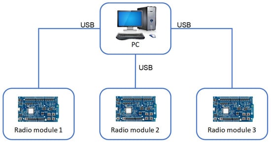
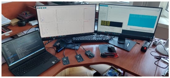
Figure 5.
Validation process test bench.
To measure the amount of energy consumed by each node in the network, the current drawn by a single node was measured. A Power Profiler Kit NRF6707 (Nordic Semiconductor, Trondheim, Norway) current measurement module was used to measure the current of each node via an NRF Connect application (Figure 6).
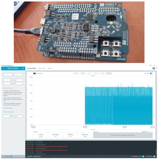
Figure 6.
Current measurement with the Power Profiler Kit.
During the algorithm validation process, the values of each criterion were measured; the results are shown in Figure 7.
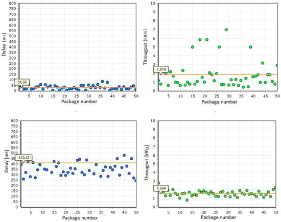
Figure 7.
Packet arrival time to destination and network throughput—data for a single packet transmitted from a NODE node to a SINK node.
Similar results were obtained for each implemented algorithm. The average current consumed by a network node was similar for each algorithm at around 1 mA, with the network nodes with the modified bee algorithm implemented showing the lowest power consumption. The average packet arrival time to the destination node was less than 100 ms, and for most packets it was less than 50 ms (the average time and throughput values are shown on the orange lines in the graphs in Figure 7). The shortest packet arrival times to the destination were obtained for the ant-based algorithm and the particle swarm optimisation algorithm.
In the functional tests, the correct functioning of the validation environment was observed. The implementation of the ACO and BEE algorithms requires the acquisition and storage of data on routes, neighbours and network parameters. In small networks of three nodes, this is not a problem. However, in larger networks, the simple microcontrollers used in NODE nodes may not be sufficient in terms of available memory and computing power, especially due to their low power consumption. It is therefore envisaged in the next stage to implement the PSO algorithm using elements of the ACO algorithm in a network consisting of a larger number of nodes.
6. Subsequent Modifications to Implement the Developed Algorithm
In a further step, the Algorithm 1 (SSAM—sensory swarm autonomous monitoring) was implemented into the extended sensor network. The algorithm is based on the pso algorithm and uses elements of the ant algorithm. Figure 8 and Figure 9 show the first step of the algorithm, which will allow each node (Figure 8) to select its best neighbour (Figure 9), according to the objective function.
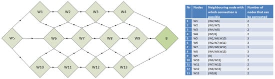
Figure 8.
Example network structure.
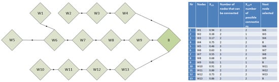
Figure 9.
Paths taken by packets after the first iteration of the routing algorithm.
In the first stage of network initialisation, NODE-type nodes send broadcast messages informing about their state to neighbouring nodes (i.e., nodes within their radio range). Information is transmitted about the state of the battery, the number of hops to the SINK node and the RSSI signal power level. At the same time, each node receives information about its neighbours and transmits it to the SINK node. The SINK node, analysing information about all nodes in the network and their neighbours, carries out the various procedures involved in the swarm algorithm. In the first phase, the position and velocity are randomly determined in the range from 0 to 1. Depending on the new position calculated according to the routing algorithm, the neighbouring node to which the data will be sent is determined (see Figure 9).
| Algorithm 1. SSAM: The Pseudocode of the algorithm is as follows |
| Initialisation: 1. Initialise the parameters of the PSO algorithm, such as number of particles, number of iterations, weighting co-factors, etc. 2. Initialise the pheromone values for each node in the sensory network. 3. Randomly initialise the positions of Pi particles in a D-dimensional space, where D is the number of nodes in the sensory network. For each iteration until the stop condition is reached: 4. For each Pi particle: a. Calculate the objective function for the current position of the Pi particle based on the sensory network. b. If the objective function is better than the best value found so far, update the particle’s best position. c. For each neighbouring node with a Pi particle, update the pheromone weights based on the ACO algorithm. 5. For each Pi particle: a. Update the particle’s velocity and position according to the equations of the PSO algorithm. 6. For a SINK node: a. Calculate for each neighbouring node the index of the target node based on its number of neighbours and the position of the Pi particle. b. Select a suitable neighbour based on the calculated index. c. Pass the information about the selected neighbour to the NODE nodes that send data to the respective SINK node. Stop condition: 7. Check the stop condition, e.g., reaching the maximum number of iterations or the set value of the objective function. Return the best particle position found, which corresponds to the optimal sensory network configuration. |
In step 6a, for a SINK node, we calculate the index of the target node based on the number of its neighbours and the position of the Pi particle. Then, in step 6b, we select the appropriate neighbour based on the calculated index. In step 6c, we pass the information about the selected neighbour to the NODE-type nodes, which then send the data to the respective SINK node. This procedure ensures that the information about the selected neighbour is passed to the NODE-type nodes. Currently, the network data path determination procedure is activated at specific time intervals, which are configurable. The main algorithmic calculations are performed in a SINK node, which can be connected to the mains power supply (and therefore has a high computing power).
7. Implementation in the Extended Network
Figure 10 illustrates a test bed designed for a network with an increased number of nodes. Tests are planned for a network of 30 nodes. The decision to use at least 20 nodes was related to the results of simulation analyses, which showed statistically significant changes in the values of the individual criteria by which the algorithms were evaluated, only at this number of nodes. The limitation of the number of physical nodes to 30 is due to the project budget that made the testing possible.
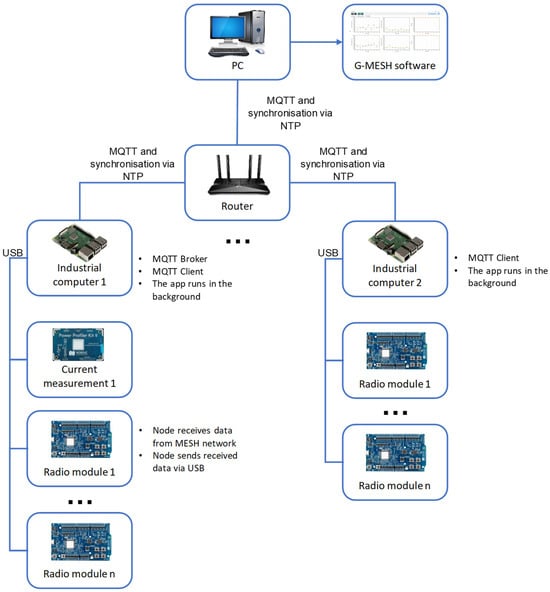
Figure 10.
Proposed test bench for more nodes.
The network was connected according to the diagram shown in Figure 11. Up to four network nodes could be connected to each Raspberry Pi computer. Diagnostic data from each node were sent via serial protocol to the Raspberry Pi computer, and then wirelessly (MQTT protocol) the data were sent to the GMESH application installed on the PC.
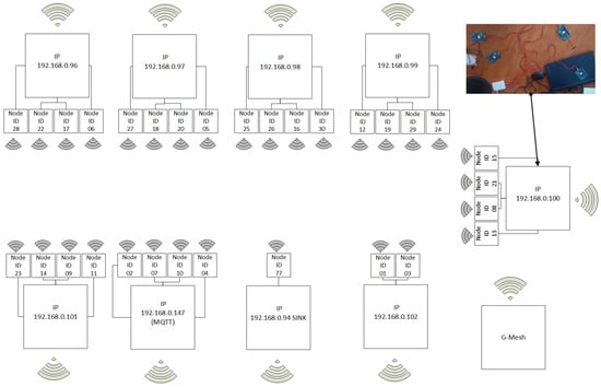
Figure 11.
Connection diagram of a sensor network for 30 nodes.
Data were recorded for a network of 10, 15, 20, 25 and 30 nodes. Figure 12 shows some of the recorded data paths for a network of 30 nodes. Note that the graphics of each node do not correspond to their physical locations. They are only used to give a quick interpretation of the path taken by the data packet.
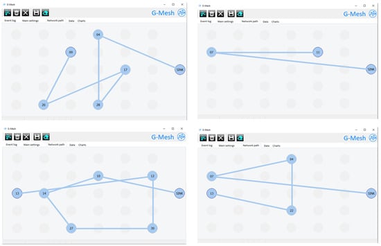
Figure 12.
Packet path in a sensor network consisting of 30 nodes.
It was observed that, despite the proximity of a node, the data in some cases were being sent to further-away nodes (in the case of close distances between nodes, about a few centimetres, —due to the determination of the distance between nodes based on the transmit power of the neighbour’s RSSI radio signal—interpreting the distance based on this signal for close distances can result in greater inaccuracy). However, in the case of close node distances, this has a negligible impact on the delivery time of the packet to the destination. Furthermore, if it is necessary to determine the distance with an accuracy of 1 cm, it is possible to implement additional modules using the UWB (ultra-wideband) radio signal in the nodes of the network.
Figure 13 shows the dependence of the recorded parameters on the number of nodes in the network. The average values of the parameters and their recorded maximum and minimum are shown.
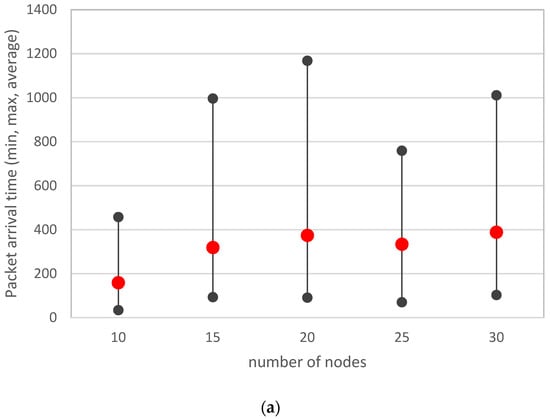
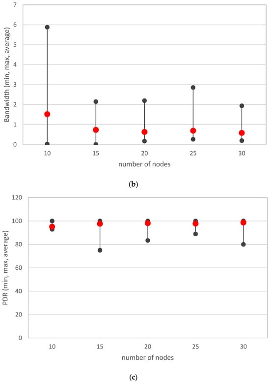
Figure 13.
Recorded parameters depending on the number of nodes in the network ((a)—packet arrival time; (b)—bandwidth; (c)—PDR).
It has been observed that as the number of nodes increases, the time it takes for a packet to reach its destination increases. This reduces the network throughput and also decreases the value of the PDR parameter (reliability of data delivery to the destination). However, the implemented algorithm makes it possible to limit the variation of the recorded parameters. For a network of 20 to 30 nodes, small differences in the recorded parameters are already visible.
8. Discussion
The integration of wireless sensor networks in mining systems is rapidly progressing, covering a variety of applications such as pressure sensing, environmental telemetry and longwall monitoring.
This paper presents the process of implementing the routing algorithm in a sensor network operating in powered roof supports, being an important component of longwall mining systems.
The assumptions for the design process of a wireless sensor network equipped with inclinometers, oil pressure sensors and distance measuring modules, meeting stringent safety standards in accordance with the ATEX directive, are presented. Given the impracticality of cable connections in dynamic mining environments, the sensors operate wirelessly with battery power, which requires optimised energy consumption to extend their functionality.
The authors conducted a simulation analysis of the routing algorithms. Reactive, proactive and swarm intelligence-based algorithms such as PSO, ACO and BEE were compared. The analysis demonstrated the ability of the algorithms to effectively manage data flow over a wide-area network infrastructure. The results showed that algorithms based on metaheuristics, such as PSO, ACO and BEE, can adapt communication routes more flexibly under dynamic environmental conditions.
The rest of the paper focused on the implementation of the selected algorithms in real hardware units. Functional tests confirmed the correctness of the algorithms, and the results showed their ability to minimise energy consumption and reduce data delivery time to the target. The next iteration of the algorithm implementation used a PSO with ACO elements, which allowed the optimisation of the communication route in the sensory network. This implementation yielded promising results, indicating the potential of the algorithm to efficiently manage sensor networks in industrial settings.
While challenges such as node replacement and network reconfiguration remain to be solved, this study provides a solid foundation for future research to improve the reliability and scalability of wireless sensor networks in mining applications. Using swarm intelligence and advanced routing algorithms, these networks promise to revolutionise safety and performance standards in underground mining operations.
Author Contributions
Conceptualization, J.J., K.S., M.H. and J.R.-R.; methodology, J.J., S.B., A.D. and M.H.; software, J.J, S.B. and J.R.-R.; validation, J.J., S.B. and J.R.-R.; formal analysis, K.S., A.D., M.H. and J.R.-R.; investigation, J.J., S.B., K.S., M.H. and J.R.-R.; resources, J.J., J.R.-R., K.S., M.H. and A.D.; data curation, J.J., S.B., M.H. and J.R.-R.; writing—original draft preparation, J.J., S.B., K.S., M.H. and J.R.-R.; writing—review and editing, J.J., S.B. and J.R.-R.; visualization, J.J. and J.R.-R.; supervision, K.S., M.H. and A.D.; project administration, J.J., S.B. and J.R.-R. All authors have read and agreed to the published version of the manuscript.
Funding
This research received no external funding.
Institutional Review Board Statement
Not applicable.
Informed Consent Statement
Not applicable.
Data Availability Statement
The data presented in this study are available in the article.
Conflicts of Interest
The authors declare no conflicts of interest.
References
- Onu, P.; Anup, P.; Charles, M. Industrial internet of things (IIoT): Opportunities, challenges, and requirements in manufacturing businesses in emerging economies. Procedia Comput. Sci. 2023, 217, 856–865. [Google Scholar]
- Szelka, M.; Woszczyński, M.; Jagoda, J.; Kamiński, P. Wireless Leak Detection System as a Way to Reduce Electricity Consumption in Ventilation Ducts. Energies 2021, 14, 3774. [Google Scholar] [CrossRef]
- Jasiulek, D.; Bartoszek, S.; Perůtka, K.; Korshunov, A.; Jagoda, J.; Płonka, M. Shield Support Monitoring System—Operation during the support setting. Acta Montan. Slovaca 2019, 4, 391–401. [Google Scholar]
- Kianfar, A.-E.; Sherikar, M.; Gilerson, A.; Skóra, M.; Stankiewicz, K.; Mitra, R.; Clausen, E. Designing a Monitoring System to Observe the Innovative Single-Wire and Wireless Energy Transmitting Systems in Explosive Areas of Underground Mines. Energies 2022, 15, 576. [Google Scholar] [CrossRef]
- Bałaga, D.; Walentek, A.; Nieradzik, P. Universal disinfecting installation UMID for decontamination of viruses, bacteria and fungi. Min. Mach. 2021, 4, 61–70. [Google Scholar] [CrossRef]
- Malec, M.; Stańczak, L. Innovative Mining Techniques and Technologies—Review of Selected KOMTECH-IMTech 2019 Conference Proceedings—Part 2. Min. Mach. 2020, 2, 13–25. [Google Scholar] [CrossRef]
- Woszczyński, M.; Rogala-Rojek, J.; Stankiewicz, K. Advancement of the Monitoring System for Arch Support Geometry and Loads. Energies 2022, 15, 2222. [Google Scholar] [CrossRef]
- Bartoszek, S.; Stankiewicz, K.; Kost, G.; Ćwikła, G.; Dyczko, A. Research on Ultrasonic Transducers to Accurately Determine Distances in a Coal Mine Conditions. Energies 2021, 14, 2532. [Google Scholar] [CrossRef]
- Bałaga, D.; Kalita, M.; Siegmund, M.; Nieśpiałowski, K.; Bartoszek, S.; Bortnowski, P.; Ozdoba, M.; Walentek, A.; Gajdzik, B. Determining and Verifying the Operating Parameters of Suppression Nozzles for Belt Conveyor Drives. Energies 2023, 16, 6077. [Google Scholar] [CrossRef]
- Rzychczy, E.; Szpyrka, M.; Korski, J.; Nalepa, G.J. Imperative vs. Declarative Modeling of Industrial Process. The Case Study of the Longwall Shearer Operation. IEEE Access 2023, 11, 54495–54508. [Google Scholar] [CrossRef]
- Stankiewicz, K. Mining control systems and distributed automation. J. Mach. Constr. Maint. 2018, 2, 117–122. [Google Scholar]
- Brandão, A.S.; Lima, M.C.; Abbas, C.J.B.; Villalba, L.J.G. An Energy Balanced Flooding Algorithm for a BLE Mesh Network. IEEE Access 2020, 8, 97946–97958. [Google Scholar] [CrossRef]
- Guolin, T.; Kaijin, Q.; Qunchao, Y. A routing layer number generation and dynamic routing algorithm on random wireless sensor network. In Proceedings of the IEEE 5th International Conference on Software Engineering and Service Science, Beijing, China, 27–29 June 2014; pp. 1052–1055. [Google Scholar]
- Şehitoğlu, A.; Aghayeva, C. Comparison of Optimal Solutions of Clusters Created Using Clustering Algorithm with Meta-Heuristic Algorithms in Capacity Vehicle Routing Problem. In Proceedings of the 2023 5th International Conference on Problems of Cybernetics and Informatics (PCI), Baku, Azerbaijan, 28–30 August 2023; pp. 1–3. [Google Scholar]
- Jagoda, J.; Hetmańczyk, M.; Stankiewicz, K. Dispersed, self-organizing sensory networks supporting the technological processes. Min. Mach. 2021, 2, 13–23. [Google Scholar] [CrossRef]
- Dyczko, A.; Kamiński, P.; Jarosz, J.; Rak, Z.; Jasiulek, D.; Sinka, T. Monitoring of Roof Bolting as an Element of the Project of the Introduction of Roof Bolting in Polish Coal Mines—Case Study. Energies 2022, 15, 95. [Google Scholar] [CrossRef]
- Jasiulek, D.; Skóra, M.; Jagoda, J.; Jura, J.; Rogala-Rojek, J.; Hetmańczyk, M. Monitoring the Geometry of Powered Roof Supports—Determination of Measurement Accuracy. Energies 2023, 16, 7710. [Google Scholar] [CrossRef]
- Bartoszek, S.; Rogala-Rojek, J.; Jasiulek, D.; Jagoda, J.; Turczyński, K.; Szyguła, M. Analysis of the Results from In Situ Testing of a Sensor In-Stalled on a Powered Roof Support, Developed by KOMAG, Measuring the Tip to Face Distance. Energies 2021, 14, 8541. [Google Scholar] [CrossRef]
- Di Renzone, G.; Fort, A.; Mugnaini, M.; Pozzebon, A.; Vignoli, V. Data Transmission from ATEX Boxes by Means of LoRa Technology for Industrial Internet of Things (IIoT) Applications. In Proceedings of the IEEE International Instrumentation and Measurement Technology Conference (I2MTC), Glasgow, UK, 17–20 May 2021; pp. 1–6. [Google Scholar]
- Smolarek, A.; Malinowski, T. Routing protocols in ad hoc networks. In Proceedings of the Teleinformatics Systems and Networks Conference 2012, Warsaw, Poland, 10–13 September 2012; pp. 47–60. [Google Scholar]
- Stankiewicz, K.; Jagoda, J.; Tonkins, M. Intelligent algorithms for routing sensory networks operating in explosion hazard zones. Min. Sci. 2021, 28, 103–115. [Google Scholar] [CrossRef]
- Lalar, S.; Yadav, A.K. Comparative study of routing protocols in MANET. Orient. J. Comput. Sci. Technol. 2017, 10, 174–179. [Google Scholar] [CrossRef]
- Chan, F.T.S.; Tiwari, M.K. Swarm Intelligence, Focus on Ant and Particle Swarm Optimization; I-Tech Education and Publishing: Rijeka, Croatia, 2007. [Google Scholar]
- Shin, C.; Lee, M. Swarm-Intelligence-Centric Routing Algorithm for Wireless Sensor Networks. Sensors 2020, 20, 5164. [Google Scholar] [CrossRef] [PubMed]
- Di Caro, G.; Ducatelle, F.; Gamberdella, L.M. Swarm intellegence for routing in mobile ad hoc networks. In Proceedings of the IEEE Swarm Intelligence Sympodium, Pasadena, CA, USA, 8–10 June 2005. [Google Scholar] [CrossRef]
- Kennedy, J.; Eberhard, R. Particle Swarm Optimization. In Proceedings of the IEEE International Conference on Neural Networks, Perth, WA, Australia, 27 November–1 December 1995; Volume 4, pp. 1942–1948. [Google Scholar]
- Kuila, P.; Jana, P.K. Energy efficient clustering and routing algorithms for wireless sensor networks: Particle swarm optimization approach. Eng. Appl. Artif. Intell. 2014, 33, 127–140. [Google Scholar] [CrossRef]
- Zungeru, A.M.; Ang, L.M.; Seng, K.P. Classical and swarm intelligence based routing protocols for wireless sensor networks. A survey and comparison. J. Netw. Comput. Appl. 2012, 35, 1508–1536. [Google Scholar] [CrossRef]
- Wedde, F. BeeAdHoc: An Energy Efficient Routing Algorithm for Mobile Ad Hoc Networks Inspired by Bee Beahavior. In Proceedings of the Genetic and Evolutionary Computation Conference, GECCO 2005, Washington, DC, USA, 25–29 June 2005. [Google Scholar]
- Praveena, K.S.; Bhargavi, K.; Yogeshwari, K.R. Comparision of PSO Algorithm and Genetic Algorithm in WSN using NS-2. In Proceedings of the International Conference on Current Trends in Computer, Electrical, Electronics and Communication (CTCEEC), Mysore, India, 8–9 September 2017; pp. 513–516. [Google Scholar] [CrossRef]
- Latiff, N.M.A.; Tsimenidis, C.C.; Sharif, B.S. Energy-Aware Clustering for Wireless Sensor Networks using Particle Swarm Optimization. In Proceedings of the IEEE 18th International Symposium on Personal, Indoor and Mobile Radio Communications, Athens, Greece, 3–7 September 2007; pp. 1–5. [Google Scholar] [CrossRef]
- Kharati, E. Using PSO and ABC Routing Algorithms Reducing Consumed Energy in Underwater Wireless Sensor Networks. Iran. J. Sci. Technol. Trans. Electr. Eng. 2022, 46, 367–380. [Google Scholar] [CrossRef]
- Ghawy, M.Z.; Amran, G.A.; AlSalman, H.; Ghaleb, E.; Khan, J.; AL-Bakhrani, A.A.; Alziadi, A.M.; Ali, A.; Ullah, S.S. An Effective Wireless Sensor Network Routing Protocol Based on Particle Swarm Optimization Algorithm. Wirel. Commun. Mob. Comput. 2022, 2022, 8455065. [Google Scholar] [CrossRef]
- Sun, W.; Tang, M.; Zhang, L.; Huo, Z.; Shu, L.A. Survey of Using Swarm Intelligence Algorithms in IoT. Sensors 2020, 20, 1420. [Google Scholar] [CrossRef] [PubMed]
- Wang, J.; Gao, Y.; Liu, W.; Sangaiah, A.K.; Kim, H.J. An Improved Routing Schema with Special Clustering Using PSO Algorithm for Heterogeneous Wireless Sensor Network. Sensors 2019, 19, 671. [Google Scholar] [CrossRef] [PubMed]
- Sahoo, B.M.; Amgoth, T.; Pandey, H.M. Particle swarm optimization based energy efficient clustering and sink mobility in heterogeneous wireless sensor network. Ad Hoc Netw. 2020, 106, 102237. [Google Scholar] [CrossRef]
- Kanchan, P.; Pushparaj, S.D. A quantum inspired PSO algorithm for energy efficient clustering in wireless sensor networks. Cogent Eng. 2018, 5, 1522086. [Google Scholar] [CrossRef]
- Lin, J.S.; Wu, S.H. A PSO-based Algorithm with Subswarm Using Entropy and Uniformity for Image Segmentation. In Proceedings of the Sixth International Conference on Genetic and Evolutionary Computing, Kitakyushu, Japan, 25–28 August 2012; pp. 500–504. [Google Scholar]
- Cai, W.; Jin, X.; Zhang, Y.; Chen, K.; Wang, R. ACO based qos routing algorithm for wireless sensor networks. In Ubiquitous Intelligence and Computing, Proceedings of the Third International Conference, UIC, Wuhan, China, 3–6 September 2006; Springer: Berlin/Heidelberg, Germany, 2006; pp. 419–428. [Google Scholar]
- Daanoune, I.; Baghdad, A.; Balllouk, A. A comparative study between ACO-based protocols and PSO-based protocols in WSN. In Proceedings of the 7th Mediterranean Congress of Telecommunications (CMT), Fez, Morocco, 24–25 October 2019; pp. 1–4. [Google Scholar] [CrossRef]
- Anand, S.; Rachitha, H.N. Enhancing Energy Efficiency Routing Protocol for Wireless Sensor Network Using ACO Algorithm. In Proceedings of the IEEE North Karnataka Subsection Flagship International Conference (NKCon), Vijaypur, India, 20–21 November 2022; pp. 1–5. [Google Scholar]
- Wu, X.; Yan, J.; Zhao, J. Comparative Research on Reactive Power Optimization of Distribution Network Based on Ant Colony and Bee Colony Algorithm. In Proceedings of the IEEE 6th Information Technology and Mechatronics Engineering Conference (ITOEC), Chongqing, China, 4–6 March 2022; pp. 247–251. [Google Scholar]
- Zhang, Q.; Wei, S.; Xue, M.; Jin, X.; Jin, C.; Li, W. A Variable-step Two Synchronous Artificial Bee Colony Algorithm for mobile Robot Path Planning. In Proceedings of the Chinese Automation Congress (CAC), Xi’an, China, 30 November–2 December 2018; pp. 2054–2058. [Google Scholar]
Disclaimer/Publisher’s Note: The statements, opinions and data contained in all publications are solely those of the individual author(s) and contributor(s) and not of MDPI and/or the editor(s). MDPI and/or the editor(s) disclaim responsibility for any injury to people or property resulting from any ideas, methods, instructions or products referred to in the content. |
© 2024 by the authors. Licensee MDPI, Basel, Switzerland. This article is an open access article distributed under the terms and conditions of the Creative Commons Attribution (CC BY) license (https://creativecommons.org/licenses/by/4.0/).