STFEformer: Spatial–Temporal Fusion Embedding Transformer for Traffic Flow Prediction

Featured Application

In the realm of Intelligent Transportation Systems, accurate prediction of traffic flow is paramount for optimizing traffic management and enhancing road safety. Our research addresses the critical challenge of capturing and modeling the complex spatial–temporal correlations inherent in traffic data. While recent advancements have seen the deployment of Spatial–Temporal Graph Neural Networks (STGNNs) and transformer models to tackle this issue, our study identifies and overcomes significant limitations in existing methodologies.

Abstract

In the realm of Intelligent Transportation Systems (ITSs), traffic flow prediction is crucial for multiple applications. The primary challenge in traffic flow prediction lies in the handling and modeling of the intricate spatial–temporal correlations inherent in transport data. In recent years, many studies have focused on developing various Spatial–Temporal Graph Neural Networks (STGNNs), and researchers have also begun to explore the application of transformers to capture spatial–temporal correlations in traffic data. However, GNN-based methods mainly focus on modeling spatial correlations statically, which significantly limits their capacity to discover dynamic and long-range spatial patterns. Transformer-based methods have not sufficiently extracted the comprehensive representation of traffic data features. To explore dynamic spatial dependencies and comprehensively characterize traffic data, the Spatial–Temporal Fusion Embedding Transformer (STFEformer) is proposed for traffic flow prediction. Specifically, we propose a fusion embedding layer to capture and fuse both native information and spatial–temporal features, aiming to achieve a comprehensive representation of traffic data characteristics. Then, we introduce a spatial self-attention module designed to enhance detection of dynamic and long-range spatial correlations by focusing on interactions between similar nodes. Extensive experiments conducted on three real-world datasets demonstrate that STFEformer significantly outperforms various baseline models, notably achieving up to a 5.6% reduction in Mean Absolute Error (MAE) on the PeMS08 dataset compared to the next-best model. Furthermore, the results of ablation experiments and visualizations are employed to clarify and highlight our model’s performance. STFEformer represents a meaningful advancement in traffic flow prediction, potentially influencing future research and applications in ITSs by providing a more robust framework for managing and analyzing traffic data.

1. Introduction

In the contemporary era of rapid urbanization, the limitations of current urban traffic management systems are becoming glaringly evident. Issues such as frequent traffic jams, ineffective congestion management, and delayed emergency response times not only hinder daily commutes but also pose significant challenges to sustainable urban development. Intelligent Transportation Systems (ITSs), as indivisible components of today’s smart urban environments [1], are instrumental in analyzing, managing, and improving traffic conditions. Within the realm of ITSs, the domain of traffic flow prediction, recognized as a pivotal technology [2], has garnered extensive research attention. This research is primarily directed towards the development of predictive models that predict future traffic flow by leveraging historical data. The precise predictions generated by these models find application in a diverse array of traffic-related domains [3], encompassing route optimization, vehicular scheduling strategies, and effective congestion alleviation measures. Accurate traffic flow predictions not only improve traffic management but also contribute to broader societal benefits, such as reduced environmental pollution, significant economic savings by decreasing time spent in traffic, and enhanced quality of life through less stressful commuting experiences. Therefore, we propose a novel traffic flow prediction model designed to comprehensively explore the spatial–temporal characteristics of traffic data and achieve accurate traffic flow prediction.

Predicting traffic flow represents a quintessential challenge in the realm of spatial–temporal data forecasting. Traffic data are captured at predetermined intervals and at distinct locations within a continuous spatial framework. Evidently, observations at neighboring locations and sequential time intervals are not isolated but dynamically interconnected. The principal challenge is effectively capturing and modeling the intricate spatial–temporal dependencies inherent in traffic data [4]. A multitude of studies have endeavored to develop diverse deep-learning models to tackle this task. Initially, several studies employed convolutional neural networks (CNNs) to analyze traffic data based on grid structures to capture spatial correlations [5,6]. Subsequently, graph neural networks (GNNs) demonstrated their suitability to model underlying graph structures [7,8]; thus, the methods based on GNNs have been extensively investigated for traffic flow prediction [9,10,11,12,13,14,15,16,17,18,19,20,21,22,23,24]. Considering the handling of temporal correlations, these GNN models primarily fall into two categories: RNN-based and CNN-based models. RNN-based methods, utilizing RNNs and their variants, such as GRUs, capture the temporal correlations in traffic data. Approaches utilizing convolutional neural networks (CNNs) capture the temporal dependencies either through a temporal convolutional network (TCN) or a standard CNN. Details are shown in

Table 1. Summary of GNN studies for traffic flow prediction.

Study	Spatial Component	Temporal Component
[9]	GNN	GRU
[10]	GNN	GRU
[11]	GNN	GRU
[12]	GNN	GRU
[13]	GNN	GRU
[14]	GNN	GRU
[15]	GNN	CNN
[16]	GNN	CNN
[17]	GNN	CNN
[18]	GNN	TCN
[19]	GNN	CNN
[20]	GNN	TCN
[21]	GNN	GRU
[22]	GNN	TCN
[23]	GNN	CNN
[24]	GNN	TCN

. However, RNNs face challenges in effectively learning long-term temporal dependencies, often failing to provide accurate predictions for extended time series. Similarly, CNNs are constrained by their limited receptive fields and local biases, which prevent them from capturing long-term temporal correlations. Additionally, the modeling of spatial correlations using existing GNN methods tends to be static, whereas in traffic systems, spatial dependencies between locations are highly dynamic and change over time due to diverse travel patterns and unforeseen events. Furthermore, these GNN models also suffer from over-smoothing as the network depth increases, which limits their ability to learn spatial correlations from a long-range perspective.

Moreover, several studies have utilized embedding structures to discover both temporal and spatial features with the goal of efficiently capturing spatial–temporal dependencies. Adaptive Graph Convolutional Recurrent Networks (AGCRNs) [9] are known to constitute a pioneering approach that designs embeddings for each node, thus creating an adaptive graph as opposed to a predefined one, establishing spatial connections and capturing spatial correlations. Both MTGNNs [15] and GMANs [25] utilize spatial embeddings to explore spatial dependencies, and GMANs additionally construct temporal embeddings through one-hot encoding, integrating them with an encoder–decoder architecture. The Adaptive Graph Spatial–Temporal Transformer Network (ASTTN) [26] also obtains temporal embeddings using one-hot encoding and obtains Laplacian positional encoding through the eigenvalue decomposition of the input graph. In addition, other models [27,28,29,30,31,32,33,34,35,36,37] also demonstrate commendable performance in traffic flow prediction. Details are shown in

Table 2. Summary of the embedding structures for traffic flow prediction.

Study	Spatial Embedding	Temporal Embedding		Native Embedding
		Short-Term	Periodic	Native Feature	Positional Encoding
[27]	√		√
[28]	√		√
[29]					√
[30]	√		√
[31]	√				√
[32]			√		√
[33]	√		√	√
[34]	√				√
[35]			√		√
[36]				√
[37]			√		√

. However, there is a lack of comprehensiveness in feature representation when constructing embedding structures. For example, the extraction of native information from traffic data is frequently neglected. The sole utilization of one-hot encoding for representing the day of the week and the time of day of each time step for the purpose of obtaining temporary embeddings falls short of effectively capturing the short-term correlations in traffic data.

To effectively explore dynamic spatial–temporal patterns and comprehensively characterize traffic data, this paper introduces a spatial–temporal fusion embedding transformer model, namely, STFEformer. As a pivotal technical contribution, we have developed a novel embedding layer aimed at processing traffic data from multiple perspectives to explore native and spatial–temporal features. Furthermore, we propose a spatial self-attention module based on the graph-masking method, designed to highlight interactions between similar nodes and capture dynamic, long-range spatial dependencies. We also employ a temporal self-attention module to discover the dynamic temporal dependencies in traffic data. In conclusion, the main contributions of this research can be summarized as follows:

• We propose STFEformer, a novel transformer-based architecture designed for precise traffic flow prediction, integrating a fusion embedding layer with spatial–temporal self-attention layers. The fusion embedding layer effectively captures native, temporal (both short-term and periodic), and spatial characteristics of traffic data. Subsequently, we utilize a spatial self-attention module based on graph masking to enhance focus on relevant nodes and capture dynamic, long-range spatial correlations. This is complemented by a temporal self-attention module that facilitates the parallel processing of spatial–temporal dependencies, addressing the comprehensive, dynamic, and long-range challenges of traffic data.
• Comprehensive experiments were carried out on three real-world public traffic datasets: PEMS04, PEMS07, and PEMS08. The results of these experiments clearly indicate that our model significantly surpasses all baseline models in terms of performance. In addition, we conducted ablation experiments to systematically evaluate the impact of the different components of our model on its overall efficacy.

2. Materials and Methods

2.1. Preliminaries

Definition 1 (Traffic network). 

The traffic network is defined as a graph, $G=\left\{V,E,A\right\}$, where $V=\left\{v_1,v_2,\dots ,v_n\right\}$represents nodes with $\left|V\right|=N$, $N$ is the number of nodes, $E\subseteq V\times V$represents edges illustrating the connections between node pairs, and $A\in {ℝ}^{N\times N}$is the adjacency matrix of the traffic network, where $A_{ij}=1$ denotes a connection between node $i$ and node $j$, otherwise $A_{ij}=0$. According to the typical stability of traffic network, $G$ is assumed to be constant in this research.

Definition 2 (Traffic flow tensor). 

In the traffic network, the traffic flow of $N$ nodes at time $t$ is defined as $X_t\in {ℝ}^{N\times F}$, where $F$ represents the dimension of traffic flow features. The traffic flow tensor at all time slices, $T$, of all nodes is defined as $\mathcal{X}=\left(X_1,X_2,X_3,\cdots ,X_T\right)\in {ℝ}^{T\times N\times F}$.

The task of traffic flow prediction is to forecast future traffic flow given historical observations. Formally, given the observed traffic flow tensor, our aim is to find a function that predicts the following T′ time steps’ traffic flow from the previous T time steps’ historical observations as follows:

$$\left[X_{t-T+1},X_{t-T+2},\cdots ,X_t;G\right]\stackrel{f}{\to }\left[X_{t+1},X_{t+2},\cdots ,X_{t+T^{\prime }}\right]$$

(1)

2.2. The Architecture of STFEformer

STFEformer is a novel transformer-based architecture designed to predict traffic flow by effectively leveraging spatial–temporal traffic data dependencies. This model aims to enhance Intelligent Transportation Systems by providing accurate traffic flow predictions. Figure 1 illustrates the framework of our proposed STFEformer. STFEformer is composed of a fusion embedding layer, a series of L spatial–temporal attention (STA) layers, and an output layer. The T time steps’ traffic flow tensor is input into the fusion embedding layer, where it undergoes transformation to obtain a combined embedding feature representation and an adaptive similarity matrix, effectively extracting both native and spatial–temporal features in traffic data. Following this, the embedding result is then fed into the STA layers, further exploring dynamic and long-range spatial–temporal dependencies. Finally, traffic flow prediction results of the next T′ time steps are directly obtained from the output layer through skip connections.

2.3. Fusion Embedding Layer

The fusion embedding layer is a cornerstone of STFEformer, designed to integrate native information with spatial–temporal features comprehensively. This layer processes the traffic data to create a multi-faceted representation. Upon undergoing processing within the fusion embedding layer, the input T time steps’ traffic flow tensor is embedded into a high-dimensional representation, enhancing the model’s ability to capture complex features in traffic data. Specifically, we employ a spatial–temporal embedding mechanism which includes adaptive spatial embedding for extracting the spatial dependency and temporal embedding to capture both short-term and periodic temporal features in traffic data. Additionally, we utilize a fully connected layer and temporal positional encoding to obtain native information from raw data.

2.3.1. Adaptive Spatial Embedding

Generally, the traffic condition of a region is influenced by its surrounding areas. To adaptively mine the spatial feature of all nodes without employing predefined distance matrices or adjacency matrices, we first introduce an adaptive spatial embedding, $E_{sp}\in {ℝ}^{N\times d_{sp}}$, where $d_{sp}$ represents the dimensions of the embedding. $E_{sp}$ is randomly initialized, with each row uniquely representing the spatial embedding of each node shared across all time slices. Then, the spatial correlations among all nodes can be expressed by multiplying $E_{sp}$ with its transpose, $E_{sp}^T$. Consequently, we can define the adaptive similarity matrix as follows:

$$M_{sp}=softmax\left(PReLU\left(E_{sp}{E}_{sp}^T\right)\right)$$

(2)

The PReLU function can adaptively adjust the slope for negative inputs, unlike the fixed slope in LeakyReLU, and, compared to ReLU, it allows a slight activation of negative inputs to prevent neuron death, thus offering greater flexibility. The softmax function is employed to standardize the adaptive similarity matrix. Each row represents the similarity between the current node and all other nodes. This matrix helps in identifying and emphasizing the relationships between nodes that exhibit similar traffic patterns, improving the model’s ability to predict under varying conditions. Subsequently, the matrix will be further integrated with spatial self-attention as a mask matrix, enabling the model to dynamically explore spatial dependencies.

2.3.2. Temporal Embedding

Due to temporary occurrences (such as traffic accidents and road maintenance) or instantaneous conditions (such as weather changes), traffic flow undergoes significant short-term perturbations and oscillations, manifesting substantial and immediate impacts. To capture the short-term temporal features of traffic flow, we employ a standard convolutional layer that merges the information in the neighboring time slices as follows:

$$E_{st}=ReLU(Con{v}_1(\mathcal{X}))$$

(3)

where $E_{st}\in {ℝ}^{T\times N\times d_{st}}$ represents the short-term embedding, $d_{st}$ indicates the dimension of the short-term feature, $Con{v}_1$ represents a standard convolutional layer, and ReLU is the activation function.

Additionally, traffic flow, influenced by the daily routines and commuting patterns of people, exhibits a clear periodicity, such as peak hours in the morning and evening, as well as disparities between weekdays and weekends. Therefore, we utilize two embeddings to effectively capture the daily and weekly periodicity of traffic flow, denoted as $e_{f_d(t)}$ and $e_{f_w(t)}\in {ℝ}^{d_{pt}}$, respectively. Here, $d_{pt}$ is the dimension of the periodicity feature and $f_d$ and $f_w$ serve as functions that convert the time t into a minute index within a day (ranging from 1 to 1440) and a day index within a week (spanning from 1 to 7). Specifically, we normalize the hour, minute, and second information from traffic data to a range between 0 and 1, thus obtaining the minute index. The day index is obtained by applying one-hot encoding. We concatenate the embeddings $e_{f_d(t)}$ and $e_{f_w(t)}$ of all T time slices to obtain temporal periodic embeddings, $E_d,E_w\in {ℝ}^{T\times d_{pt}}$.

In this paper, we set the dimension $d_{st}=d_{pt}=d_t$. We obtain the temporal embedding $E_t\in {ℝ}^{T\times d_t}$ by simply summing $E_{st}$, $E_d$, and $E_w$, thereby integrating both the short-term and periodic temporal features in traffic data given as follows:

$$E_t=E_{st}+E_d+E_w$$

(4)

2.3.3. Native Feature Embedding

To preserve the native information contained within the raw data, a fully connected layer is employed to obtain token embedding, $E_{tok}\in {ℝ}^{T\times N\times d_{tok}}$, as follows:

$$E_{tok}=FC\left(\mathcal{X}\right)$$

(5)

where $d_{tok}$ is the token embedding’s dimension and $FC\left(\cdot \right)$ represents a fully connected layer.

Inspired by the positional encoding mechanism in the original transformer model [38], we designed a temporal positional encoding method to introduce essential positional information of input traffic time sequences, denoted as $E_{tpe}\in {ℝ}^{T\times d_{tpe}}$. Here, $d_{tpe}$ is the dimension of the temporal positional encoding. We utilize sine and cosine functions of different frequencies as follows:

$$\left\{\begin{array}{c}TP{E}_{\left(pos,2i\right)}=\sin \left(pos/{10000}^{2i/d_{tpe}}\right)\\ TP{E}_{\left(pos,2i+1\right)}=\sin \left(pos/{10000}^{(2i+1)/d_{tpe}}\right)\end{array}\right.$$

(6)

where pos is the time position, $i$ is the dimension, and 10,000 is the hyperparameter derived from the transformer [38].

In this work, we set the dimension $d_{tok}=d_{tpe}=d_f$. The native feature embedding, $E_f\in R^{T\times N\times d_f}$, can be obtained by summing $E_{tok}$ and $E_{tpe}$ as follows:

$${\mathrm{E}}_f{=\mathrm{E}}_{tok}{+\mathrm{E}}_{tpe}$$

(7)

2.3.4. Embedding Fusion

By concatenating the aforementioned embeddings, we can obtain the outcome of the fusion embedding layer given as follows:

$$X_{emb}=E_{sp}‖E_t‖E_f$$

(8)

Subsequently, $X_{emb}\in {ℝ}^{T\times N\times (d=d_{sp}+d_t+d_f)}$ will be input into the spatial–temporal attention layers, and $X$ is used to denote $X_{emb}$ for convenience.

2.4. Spatial–Temporal Attention Layer

Based on the multi-head self-attention mechanism, we developed a spatial–temporal attention layer to capture both dynamic and long-range spatial–temporal correlations. The attention layer is comprised of two key modules. The first, a spatial self-attention module, incorporates an adaptive similarity matrix that dynamically identifies and emphasizes the interactions between a node and others that exhibit similar traffic patterns, enhancing the model’s capacity to capture spatial dynamics. Concurrently, the temporal self-attention module is engineered to discover long-range and dynamic temporal dependencies, ensuring that important temporal information is preserved and integrated throughout the predictive process. By maintaining a continuous flow of essential spatial and temporal features, these modules collectively improve the accuracy and reliability of traffic flow predictions.

To precisely describe the operations of multi-head self-attention, we employ the following slicing symbol. In the context of an embedding, $X\in {ℝ}^{T\times N\times d}$, the slicing operation along the T-axis yields the matrix $X_{t::}\in {ℝ}^{N\times d}$, and slicing along the N-axis produces the matrix $X_{:n:}\in {ℝ}^{T\times d}$.

2.4.1. Spatial Self-Attention

In the spatial dimension, the traffic conditions at various locations interact with each other in a highly dynamic manner. To capture this dynamic spatial dependency in traffic data, we designed a spatial self-attention module.

We first calculate the query, key, and value (QKV) matrices at time t via the self-attention operation as follows:

$$Q_t^S=X_{t::}{W}_Q^S,K_t^S=X_{t::}{W}_K^S,V_t^S=X_{t::}{W}_V^S$$

(9)

where $W_Q^S$, $W_K^S$, and $W_V^S\in {ℝ}^{d\times d^{\prime }}$ denote learnable parameter matrices and d′ represents the dimension of the query, key and value (QKV) matrices. Then, we apply the spatial self-attention operation to explore the interactions among all nodes and obtain spatial correlations (attention scores) between each pair of nodes at time t as follows:

$$A_t^S=\frac{Q_t^S\times {\left(K_t^S\right)}^T}{\sqrt{d^{\prime }}}$$

(10)

It is evident that the spatial correlations, $A_t^S\in {ℝ}^{N\times N}$, between nodes vary across different time slices, and this operation takes into account the connections between all nodes. Therefore, the spatial self-attention module is able to capture long-range and dynamic spatial dependencies. Finally, by normalizing the attention scores and multiplying them with the value matrix, we obtain the output of the spatial self-attention (SSA) module given as follows:

$$SSA\left(Q_t^S,K_t^S,V_t^S\right)=softmax(A_t^S)V_t^S$$

(11)

As mentioned above, each node is involved in interactions with every other node that are equivalent considering the spatial structure in the form of a fully connected graph. However, only the interaction between a few nodes sharing similar functions is crucial. By identifying and focusing attention more on these similar nodes, the model becomes more efficient and accurate. Therefore, we transform the adaptive similarity matrix obtained from the fusion embedding layer into a graph mask matrix, integrating it with the SSA module. Specifically, we choose the top K nodes that exhibit the greatest similarity for each individual node based on the adaptive similarity matrix. By establishing the weight assigned to the edges connecting the current node with its K similar nodes as 1 and that assigned to the others as 0, we construct a binary mask matrix. Furthermore, we evolve the original SSA into MaskSSA, which can be denoted as follows:

$$MaskSSA(Q_t^S,K_t^S,V_t^S)=softmax(A_t^S\odot M_{mask})V_t^S$$

(12)

where $\odot$ denotes the Hadamard product. The spatial self-attention module can focus more on the dynamic interactions between similar nodes in this way.

Finally, we expand MaskSSA into a multi-head spatial self-attention mechanism to gain a more comprehensive understanding of the dynamic and long-range spatial dependencies, thereby enhancing the model’s generalization capabilities. The result of the spatial self-attention module can be obtained as follows:

$$Z_{MaskSSA}=MaskSS{A}_1\parallel MaskSS{A}_2\parallel \dots \parallel MaskSS{A}_{h_{ssa}}$$

(13)

where $h_{ssa}$ is the number of attention heads of the spatial self-attention module.

2.4.2. Temporal Self-Attention

In the temporal dimension, dependencies between traffic conditions across various time slices are evident, such as periodicity and trends that fluctuate in different scenarios. To adaptively capture dynamic temporal correlations, a temporal self-attention (TSA) module is utilized. Specifically, we initially calculate the query, key, and value (QKV) matrices for node n as follows:

$$Q_n^T=X_{:n:}{W}_Q^T,K_n^T=X_{:n:}{W}_K^T,V_n^T=X_{:n:}{W}_V^T$$

(14)

where $W_Q^T$, $W_K^T$, and $W_V^T\in {ℝ}^{d\times d^{\prime }}$ represent learnable parameter matrices and d′ denotes the dimension of these learnable matrices. Then, the temporal correlations (attention scores) between all time slices for node n can be obtained via the self-attention operation as follows:

$$A_n^T=\frac{Q_n^T\times {\left(K_n^T\right)}^T}{\sqrt{d^{\prime }}}$$

(15)

It is evident that the temporal self-attention module is capable of effectively exploring the temporal dynamic dependencies for diverse nodes. Furthermore, the temporal self-attention module possesses an expansive global receptive field feature, enabling it to capture long-range temporal dependencies. Then, the output of the temporal self-attention module can be obtained as follows:

$$TSA\left(Q_n^T,K_n^T,V_n^T\right)=softmax(A_n^T)V_n^T$$

(16)

Finally, we expand TSA into multi-head temporal self-attention. The output can be obtained as follows:

$$Z_{TSA}=TS{A}_1\parallel TS{A}_2\parallel \dots \parallel TS{A}_{h_{tsa}}$$

(17)

where $h_{tsa}$ is the number of attention heads of the temporal self-attention module.

2.4.3. Spatial–Temporal Attention Fusion

In order to diminish the computational complexity of the model, the heterogeneous spatial–temporal self-attention outcomes are combined after defining two types of attention modules. We concatenate the outcomes of these attention modules and then project them to yield the outputs, enabling the model to simultaneously incorporate information from spatial and temporal dimensions. Formally, the output can be obtained as follows:

$$STA=\left(Z_{MaskSSA}\parallel Z_{TSA}\right)W_f$$

(18)

where $W_f\in {ℝ}^{d\times d}$ represents a learnable projection matrix and $d^{\prime }=d/\left(h_{ssa}+h_{tsa}\right)$ is set in this paper.

Additionally, we further apply a position-wise fully connected feed-forward network. This enables the model to delve deeper into the extraction of complex and abstract characteristics in traffic data by applying two linear transformations. Formally, this network can be defined as follows:

$$X_{FFN}=GELU\left(\left(STA\right)W_1+b_1\right)W_2+b_2$$

(19)

where $X_{FFN}\in {ℝ}^{T\times N\times d}$ is the output of the network; $W_1$, $b_1$, $W_2$, and $b_2$ represent learnable parameters; and GeLU is the activation function. We also introduce residual connection and layer normalization here, as in the original transformer [38].

2.5. Output Layer

To enhance the propagation of features and gradients throughout our model and to counteract potential problems of gradient vanishing or explosion, we implement skip connections using a standard convolution layer with an $1\times 1$-sized kernel. These skip connections play a crucial role in preserving vital information from earlier layers by bypassing intermediate layers directly to later ones. This method not only facilitates a smoother and more stable training process by ensuring that gradients flow freely through the network but also helps in retaining critical information necessary for accurate prediction over long-range dependencies. By integrating these connections, our model is better equipped to produce precise and reliable traffic flow predictions, leveraging both deep and surface-level features effectively. It transforms the output, $X_{FFN}$, into $X_{skip}\in {ℝ}^{T\times N\times d_{skip}}$, where $d_{skip}$ is the skip dimension. Then, the output of each skip connection layer is summed to obtain the final hidden state, $X_{fs}\in {ℝ}^{T\times N\times d_{skip}}$. It can flexibly adjust the representational dimensions of features, ensuring their efficient propagation in the deeper layers of the network and preserving temporal and spatial features simultaneously.

To achieve multi-step traffic flow prediction, the output layer is directly employed to obtain the prediction result as follows:

$$X_{Pred}=Con{v}_3(Con{v}_2(X_{fs}))$$

(20)

where $X_{Pred}\in {ℝ}^{T^{\prime }\times N\times F}$ represents the T′ time steps’ prediction result and $Con{v}_2$ and $Con{v}_3$ are two standard convolution layers, each characterized by a kernel size of $1\times 1$. The convolution layers are used to transform the time steps and the skip dimension of $X_{fs}$, respectively. Considering cumulative errors and computational efficiency, we use a direct way instead of adopting a recursive manner to obtain prediction values.

STFEformer sets a new benchmark for the prediction of spatial and temporal traffic data in Intelligent Transportation Systems. The modular and adaptable design of STFEformer serves as a foundation for future predictive models in the field. By demonstrating how dynamic and long-range spatial–temporal correlations patterns can be effectively captured and integrated, STFEformer offers a blueprint for future developments in traffic management, urban planning, and beyond. Researchers and engineers can build upon this architecture to create more nuanced models that accommodate the increasing complexity of traffic datasets and drive advancements in real-time, adaptive traffic management systems.

3. Experiments

3.1. Datasets

The performance of STFEformer was corroborated by experimental validation on three real-world public datasets, namely, PeMS04, PeMS07, and PeMS08 [23]:

PeMS04: The traffic data were gathered by the California Transportation Agency’s (CalTrans) Performance Measurement System (PeMS) from 1 January to 28 February 2018, utilizing 307 sensors. This dataset encompasses traffic flow information, which is consolidated into intervals of every 5 min.

PeMS07: This dataset encompasses data spanning four months, acquired through 883 sensors from 1 May to 31 August 2017. It includes traffic flow information aggregated at 5 min intervals.

PeMS08: This dataset encompasses data spanning two months acquired through 170 sensors from 1 July to 31 August 2016. It includes traffic flow information aggregated at 5 min intervals.

Details are presented in

Table 3. Dataset description.

Dataset	No. of Nodes	No. of Edges	No. of Time Steps	Time Interval	Time Range
PeMS04	307	340	16,992	5 min	1 January–28 February 2018
PeMS07	883	866	28,224	5 min	1 May–31 August 2017
PeMS08	170	295	17,856	5 min	1 July–31 August 2016

. We use the past hour’s (12 time steps) data to predict the following hour’s (12 time steps) traffic flow. The dataset is partitioned into three segments: 60% allocated for training, 20% for validation, and the remaining 20% for testing.

3.2. Experimental Setups

All experiments were conducted on a machine with an NVIDIA GeForce RTX 4090 GPU and 24 GB of memory, utilizing Python 3.9.7. The embedding dimensions were set as $d_{sp}=24$, $d_t=24$, and $d_f=24$. The depth of the spatial–temporal attention layers, L, was 6. Both the input and output time steps corresponded to 1 h, i.e., $T=T^{\prime }=12$. The number of heads for both the spatial and temporal self-attention modules was 4. The learning rate was 0.001, and the batch size was 16. Adam was chosen as the optimizer. Based on the performance on the validation set, the optimal model was determined. If the validation loss converged over a span of 20 continuous steps, an early-stop mechanism was implemented.

We utilized three metrics to evaluate the predictive accuracy of the model during the experiments: Mean Absolute Error (MAE), Root Mean Square Error (RMSE), and Mean Absolute Percentage Error (MAPE). We also excluded missing values when calculating these metrics.

MAE is defined as follows:

$$MAE=\frac{1}{N}{\displaystyle \sum _{i=1}^N\left|y_i-{\widehat{y}}_i\right|}$$

(21)

RMSE is defined as follows:

$$RMSE=\sqrt{\frac{1}{N}{\displaystyle \sum _{i=1}^N{\left(y_i-{\widehat{y}}_i\right)}^2}}$$

(22)

MAPE is defined as follows:

$$MAPE=\frac{1}{N}{\displaystyle \sum _{i=1}^N\left|\frac{y_i-{\widehat{y}}_i}{y_i}\right|}\times 100\%$$

(23)

where $y_i$ is the true value and ${\widehat{y}}_i$ is the prediction result.

3.3. Baselines

We compared STFEformer with 12 baseline models. Descriptions of these baseline methods are provided as follows:

VAR [39]: Vector Auto-Regression (VAR) is a statistical model utilized for time-series data analysis. It captures the dynamic relationships between variables. In this model, each variable is represented as a linear function influenced by its own historical values as well as those of other variables, thus facilitating the simultaneous analysis of several time series.

SVR [40]: Support Vector Regression (SVR) is a regression method derived from the principles of the Support Vector Machine (SVM). The core idea of SVR is to determine a decision boundary, namely, a regression hyperplane, that maximizes the margin to the nearest training sample points.

DCRNN [7]: The Diffusion Convolutional Recurrent Neural Network (DCRNN) models traffic flow as a diffusion process in directed graphs. It introduces bidirectional random walks in the graphs to explore spatial features and utilizes an encoder–decoder architecture with Gated Recurrent Units (GRUs) to learn temporal correlations.

ASTGCN [41]: The Attention-Based Spatial–Temporal Graph Convolutional Network (ASTGCN) uses approximate expansion of Chebyshev polynomials to explore spatial dependencies and a standard convolution layer to model temporal features. Additionally, a spatial–temporal attention mechanism is employed to capture the dynamic spatial–temporal correlations in traffic data.

STSGCN [23]: The Spatial–Temporal Synchronous Graph Convolutional Network (STSGCN) introduces a novel spatial–temporal graph convolutional module that synchronizes the capture of local spatial–temporal dependencies. Additionally, a multiple-module layer was designed to explore heterogeneity in spatial–temporal graphs. It deploys multiple modules in each time period, allowing each module to concentrate on extracting the spatial–temporal dependencies from localized spatial–temporal graphs.

AGCRN [9]: The Adaptive Graph Convolutional Recurrent Network (AGCRN) designs a node adaptive parameter learning module to explore spatial features for each node. It also introduces a data adaptive graph generation module to automatically capture the intercorrelations between various tensors. Moreover, the two modules are combined with Gated Recurrent Units (GRUs) to learn temporal dependencies.

GMAN [25]: The Graph Multi-Attention Network (GMAN) proposes a spatial–temporal attention mechanism to explore dynamic spatial and non-linear temporal correlations. To adaptively fuse the outputs derived from spatial–temporal attention, gated fusion was also designed. Furthermore, it employs a transform attention mechanism to obtain prediction representations from historical features.

Z-GCNETs [42]: Time-Aware Zigzags at Graph Convolutional Networks (Z-GCNETs) is a pioneering approach that merges time-conditioned DL with time-aware persistent homology data representations. A zigzag topological layer designed specifically for time-aware graph convolutional networks was developed and integrated with Gated Recurrent Units (GRUs). This model is able not only to capture the topological attributes of data but also to comprehend how these characteristics evolve over time.

STFGNN [22]: The Spatial–Temporal Fusion Graph Neural Network (STFGNN) designs a novel adjacency matrix via row data and is capable of extracting features that spatial graphs may not reflect. Additionally, by integrating a dilated CNN module with a gated mechanism and a spatial–temporal fusion graph module, it can explore long-range and long-term spatial–temporal correlations through layer stacking.

STGODE [20]: The Spatial–Temporal Graph ODE Network (STGODE) proposes a novel ordinary differential equation based on tensor form to capture spatial–temporal dynamics. A semantical adjacency matrix was designed to comprehensively consider spatial correlations. Moreover, it also utilizes a temporal dilatated convolution structure to explore long-range temporal correlations.

DSTAGNN [21]: The Dynamic Spatial–Temporal-Aware Graph Neural Network (DSTAGNN) constructs a graph that captures dynamic attributes related to nodes by mining historical observations. Based on multi-order Chebyshev polynomials in GCNs, a novel spatial–temporal attention module was designed to explore dynamic spatial dependencies, and an enhanced gated convolution module was designed to enhance the model’s capacity to capture dynamic temporal correlations.

ASTGCNs [43]: Adaptive Spatial–Temporal Graph Convolution Networks (ASTGCNs) utilize an adaptive graph convolution along with an attention mechanism to effectively address bias present in clearly defined graph structures and explore local spatial–temporal dependency in data. It also utilizes a temporal convolution network and an ordinary differential equation module to learn global spatial–temporal dependencies.

4. Experimental Results and Discussion

4.1. Performance Comparison

Table 4. Performance comparison of STFEformer and other baseline models.

	PeMS04			PeMS07			PeMS08
Model	MAE	RMSE	MAPE	MAE	RMSE	MAPE	MAE	RMSE	MAPE
VAR	25.54	38.61	18.24%	99.20	131.14	38.69%	22.31	33.63	14.57%
SVR	28.56	43.29	19.03%	31.87	49.15	14.43%	23.15	35.25	14.69%
DCRNN	24.60	38.02	17.11%	25.20	38.55	11.64%	17.83	27.78	11.48%
ASTGCN	22.84	35.28	16.38%	27.05	40.57	12.82%	18.21	28.06	12.88%
STSGCN	21.19	33.65	13.90%	24.26	39.03	10.21%	17.13	26.80	10.96%
AGCRN	19.83	32.26	12.97%	22.17	36.12	9.17%	15.95	25.22	10.09%
Z-GCNETs	19.50	31.61	12.78%	21.73	35.07	9.25%	15.76	25.11	10.01%
STFGNN	19.83	31.88	13.02%	22.07	35.80	9.21%	16.64	26.22	10.60%
STGODE	20.84	32.82	13.77%	22.99	37.54	10.14%	16.81	25.97	10.62%
DSTAGNN	19.30	31.46	12.70%	21.42	34.51	9.01%	15.67	24.77	9.94%
ASTGCNs	20.14	31.60	13.87%	21.90	34.52	9.82%	15.99	24.90	10.21%
STFEformer	18.98	30.94	12.65%	20.50	33.87	8.75%	14.80	24.22	9.85%

presents the performance results of various models tested on three real-world datasets. These experimental results showcase the superiority of our model in comparison to all other baseline models across the entirety of the datasets.

Compared to the other baseline models, VAR and SVR exhibited inferior performance, primarily due to their sole focus on the temporal dimension while neglecting the spatial correlations inherent in traffic flow. This underscores the critical importance of considering temporal and spatial correlations simultaneously when modeling traffic flow.

In contrast, spatial–temporal deep-learning models generally demonstrated superior performance. DCRNN, ASTGCN, and STSGCN are three models that concurrently process information across both temporal and spatial dimensions. DCRNN, which is based on the RNN in the temporal dimension, encounters a limit in capturing long-range temporal correlations. ASTGCN employs a standard convolution layer to aggregate information only from neighboring time slices, which makes it difficult to gain a promising ability to model temporal dependency. In the spatial dimension, both DCRNN and ASTGCN utilize predefined adjacency matrices to learn spatial dependency. In comparison, STSGCN employs a temporal embedding matrix and a spatial embedding matrix, both of which are learnable. It also utilizes spatial–temporal convolution modules to extract features, thus enhancing performance. However, it only captures local spatial–temporal correlations, limiting its ability to discover global information in traffic flow.

Both AGCRN and Z-GCNETs utilize GRUs to learn temporal patterns, yet they fall short of efficiently capturing dynamic and long-range temporal correlations. In terms of spatial dependency learning, AGCRN and Z-GCNETs adopt distinct approaches. AGCRN learns unique parameters for each node based on matrix factorization and accordingly constructs an adaptive graph generation module capable of autonomously inferring dependencies among different traffic series. On the other hand, Z-GCNETs design time-aware graph convolutions to capture topological attributes in traffic data.

In the spatial dimension, GMAN develops a spatial embedding which is similar to AGCRN but employs a spatial attention mechanism instead of graph convolution. In the temporal dimension, it develops temporal embedding and a temporal attention mechanism. However, the embeddings are not comprehensive enough. Moreover, an encoder–decoder architecture is utilized to explore spatial–temporal correlations.

Both STFGNN and DSTAGNN rely on mining historical data to construct data-driven graph structures as opposed to using predefined graphs, thereby enhancing the exploration of previously unexposed spatial correlations. Moreover, DSTAGNN leverages an attention mechanism and a gated convolution module, augmenting its capability to capture dynamic spatial correlations. In the temporal dimension, STFGNN employs a gated dilated convolution module with extensive dilation to broaden its receptive field in time series, capturing temporal correlations. DSTAGNN introduces a multi-scale gated tanh unit to explore temporal information. Both methods lack the ability to capture dynamic temporal correlations.

Both STGODE and ASTGCN enhance performance in traffic flow prediction by integrating the structure of Ordinary Differential Equations (ODEs). Specifically, STGODE constructs a semantic adjacency matrix to capture the semantic associations between nodes via Dynamic Time Warping (DWT). It also designs a spatial–temporal graph convolution based on an ODE structure to simultaneously handle spatial and temporal information. ASTGCN, based on node-adaptive parameters, constructs an adaptive graph and further combines it with an attention mechanism to explore local spatial–temporal features. Moreover, STGODE employs two TCN blocks to extract long-range temporal correlations, while ASTGCNs adopt both TCNs and ODEs to further explore global spatial–temporal features.

Our model, STFEformer, exhibited superior prediction performance on all three real-world datasets. Specifically, on the PeMS04 dataset, STFEformer’s MAE was 18.98, surpassing the second-best model, DSTAGNN, which had an MAE of 19.30. Additionally, STFEformer presented a lower RMSE of 30.94 compared to DSTAGNN’s RMSE of 31.46, and a lower MAPE of 12.65% compared to DSTAGNN’s MAPE of 12.70%. Similarly, on the PeMS07 dataset, STFEformer achieved an MAE of 20.50, an RMSE of 33.87, and an MAPE of 8.75%, while DSTAGNN obtained an MAE of 21.42, an RMSE of 34.51, and an MAPE of 9.01%. On the PeMS08 dataset, STFEformer achieved an MAE of 14.80, an RMSE of 24.22, and an MAPE of 9.85%, while DSTAGNN exhibited an MAE of 15.67, an RMSE of 24.77, and an MAPE of 9.94%.

These improvements are attributed to the combination of short-term features and periodic features in the temporal dimension, the use of data-driven adaptive spatial embeddings without predefined graphs, and native feature extraction from raw data. Then, our model utilizes a spatial self-attention module which integrates an adaptive similarity matrix, thereby highlighting interactions between similar nodes and capturing dynamic and long-range spatial correlations. To explore dynamic temporal dependencies, a temporal self-attention module is also employed. In conclusion, our model effectively captures complex features in traffic data.

4.2. Ablation Study Results

To assess the efficacy of each component in STFEformer, ablation experiments with five variants of our model were conducted:

• w/o MaskSSA. This removes the mask spatial self-attention.
• w/o mask. This removes the binary mask matrix.
• w/o $E_{sp}$. This removes the adaptive spatial embedding, $E_{sp}$.
• w/o $E_f$. This removes the native feature embedding, $E_f$.
• w/o $E_t$. This removes the temporal embedding, $E_t$.

The experiments were carried out on the PeMS04, PeMS07, and PeMS08 datasets. The results are as shown in

Table 5. The overall 12-time-step prediction results of the ablation study.

	PeMS04			PeMS07			PeMS08
Model	MAE	RMSE	MAPE	MAE	RMSE	MAPE	MAE	RMSE	MAPE
w/o MaskSSA	20.76	33.57	13.45%	22.25	36.66	9.17%	15.55	25.43	10.32%
w/o mask	19.31	31.38	12.98%	20.75	34.37	8.93%	15.09	24.68	9.97%
w/o $E_{sp}$	21.65	34.63	13.64%	22.94	37.34	9.32%	15.70	26.25	10.38%
w/o $E_f$	20.13	35.53	13.12%	21.56	35.73	9.09%	15.39	25.11	10.22%
w/o $E_t$	21.88	35.02	13.76%	23.12	37.82	9.45%	15.95	26.58	10.45%
STFEformer	18.98	30.94	12.65%	20.50	33.87	8.75%	14.80	24.22	9.85%

,

Table 6. The next 3-, 6-, 9-, and 12-time-step prediction results of the ablation study on PeMS04.

	3			6			9			12
Model	MAE	RMSE	MAPE	MAE	RMSE	MAPE	MAE	RMSE	MAPE	MAE	RMSE	MAPE
w/o MaskSSA	19.82	31.62	12.64%	20.66	33.13	13.31%	21.42	34.33	13.89%	22.40	35.71	14.54%
w/o mask	18.28	29.55	12.20%	19.27	31.08	12.89%	19.97	32.33	13.41%	20.96	33.60	14.04%
w/o $E_{sp}$	19.33	31.06	12.78%	21.28	33.76	13.51%	22.15	36.25	14.84%	24.28	38.44	15.97%
w/o $E_f$	19.17	30.83	12.47%	20.03	32.36	13.05%	21.07	33.69	13.68%	21.41	34.32	14.26%
w/o $E_t$	19.92	31.85	12.71%	21.48	34.18	13.66%	22.64	36.81	15.18%	24.72	38.67	16.15%
STFEformer	18.00	29.30	11.95%	18.98	30.96	12.63%	19.62	32.02	13.07%	20.61	33.36	13.69%

,

Table 7. The next 3-, 6-, 9-, and 12-time-step prediction results of the ablation study on PeMS07.

	3			6			9			12
Model	MAE	RMSE	MAPE	MAE	RMSE	MAPE	MAE	RMSE	MAPE	MAE	RMSE	MAPE
w/o MaskSSA	21.02	33.39	8.62%	22.17	35.71	9.09%	23.14	37.41	9.54%	24.34	39.18	10.16%
w/o mask	19.55	31.37	8.42%	20.68	33.66	8.85%	21.58	35.28	9.23%	22.89	37.15	9.95%
w/o $E_{sp}$	20.39	33.06	8.80%	22.61	36.04	9.28%	25.18	39.96	10.03%	27.47	42.47	11.00%
w/o $E_f$	20.16	32.42	8.61%	21.46	35.47	8.95%	22.27	36.49	9.29%	23.54	38.16	10.00%
w/o $E_t$	21.00	33.74	8.75%	22.66	37.12	9.33%	25.49	40.86	10.24%	27.76	43.36	11.13%
STFEformer	19.29	30.98	8.21%	20.40	33.17	8.63%	21.37	34.85	9.08%	22.67	36.68	9.84%

and

Table 8. The next 3-, 6-, 9-, and 12-time-step prediction results of the ablation study on PeMS08.

	3			6			9			12
Model	MAE	RMSE	MAPE	MAE	RMSE	MAPE	MAE	RMSE	MAPE	MAE	RMSE	MAPE
w/o MaskSSA	14.72	23.79	9.70%	15.48	25.37	10.23%	16.34	26.53	10.77%	17.08	27.95	11.62%
w/o mask	14.17	22.93	9.20%	15.02	24.56	9.92%	15.64	25.88	10.38%	16.53	26.83	11.10%
w/o $E_{sp}$	14.82	23.17	9.65%	15.57	25.96	10.16%	17.05	27.56	11.16%	17.97	28.09	12.20%
w/o $E_f$	14.42	22.97	9.38%	15.28	25.02	9.99%	15.78	26.29	10.66%	16.79	27.11	11.24%
w/o $E_t$	14.91	23.99	9.70%	15.71	26.38	10.25%	17.31	28.06	11.34%	18.82	29.00	12.31%
STFEformer	13.88	22.43	9.13%	14.83	24.36	9.82%	15.34	25.38	10.24%	16.27	26.60	10.87%

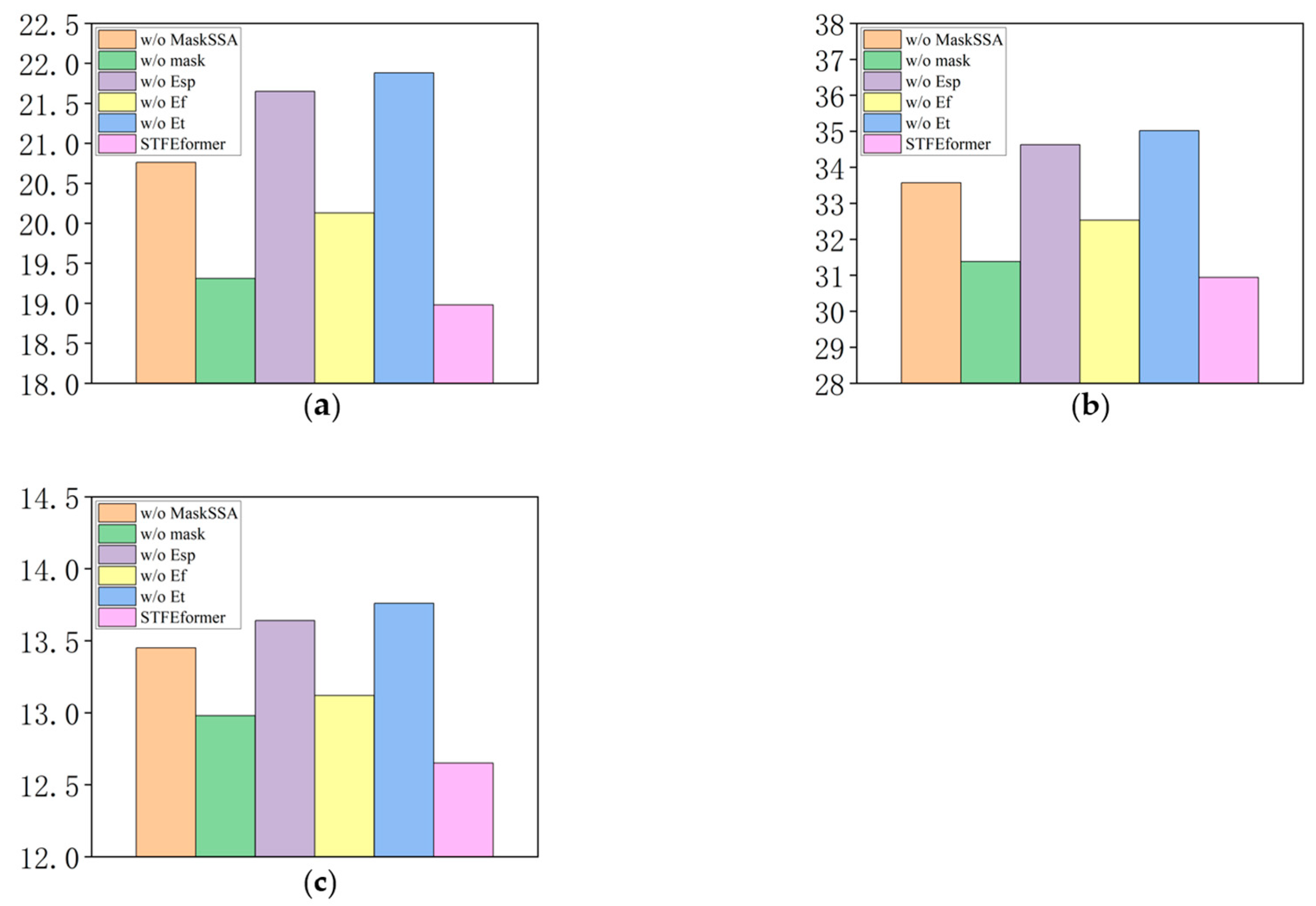
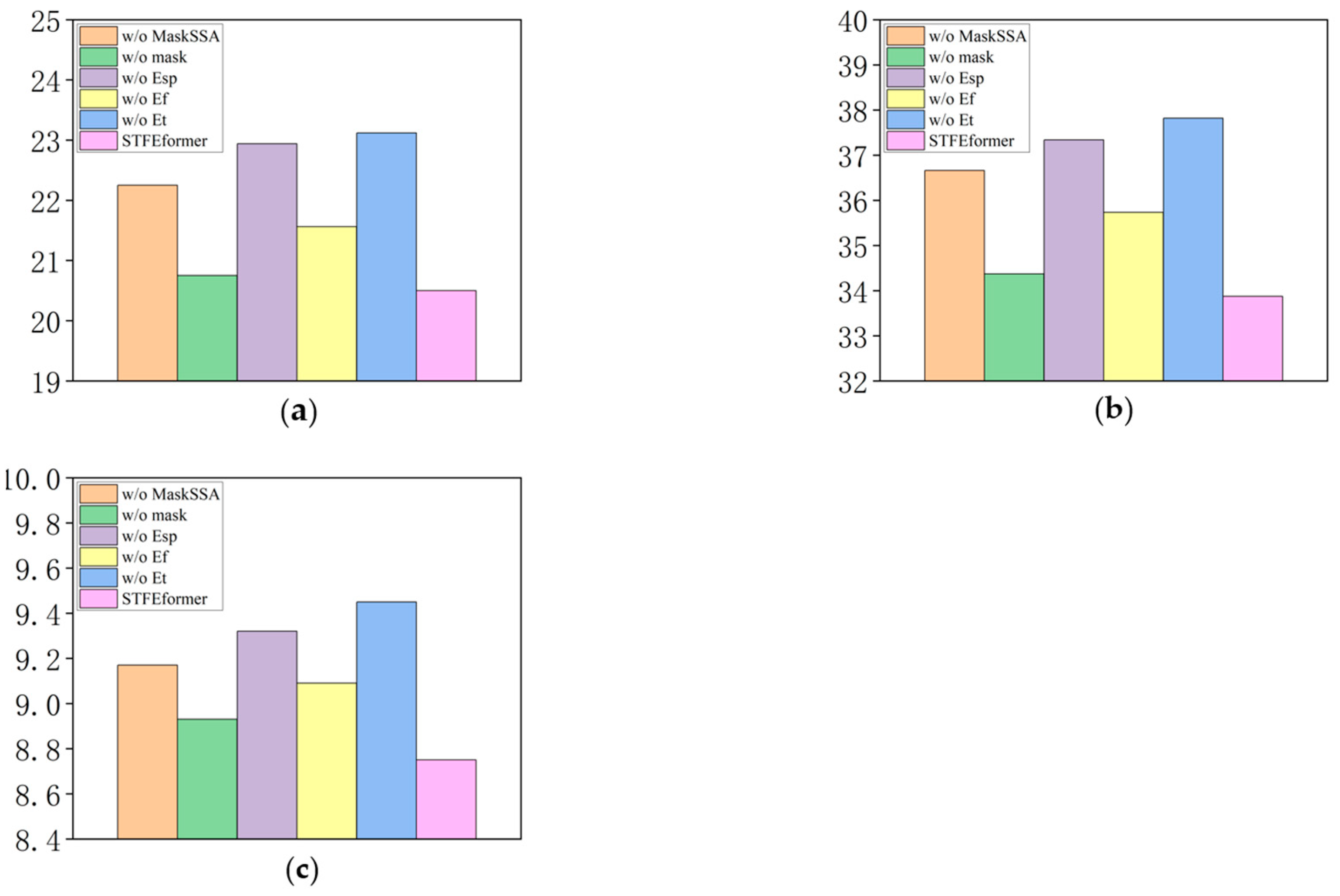
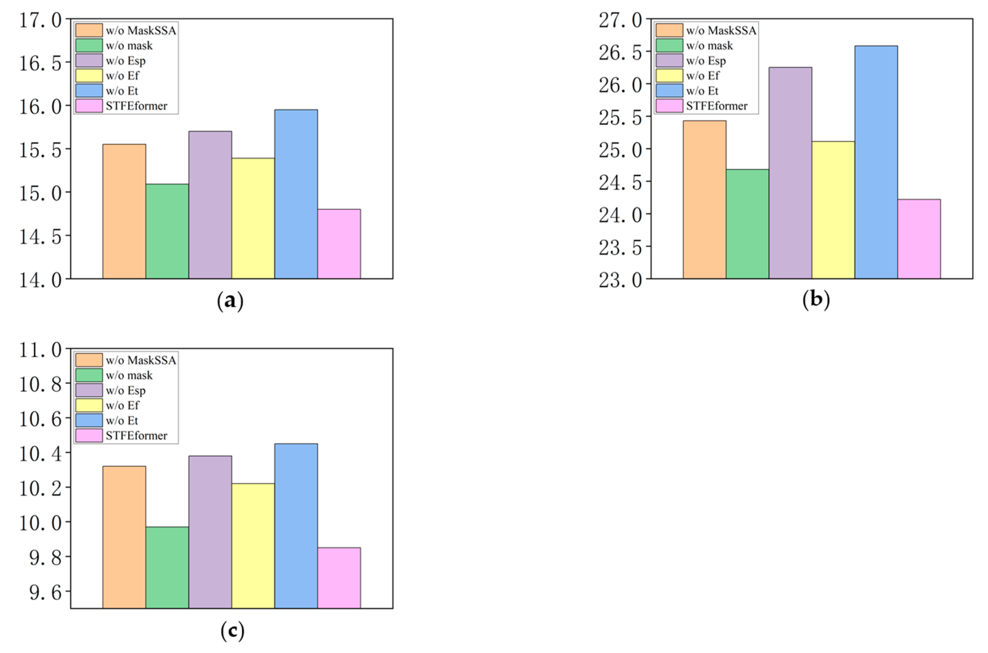
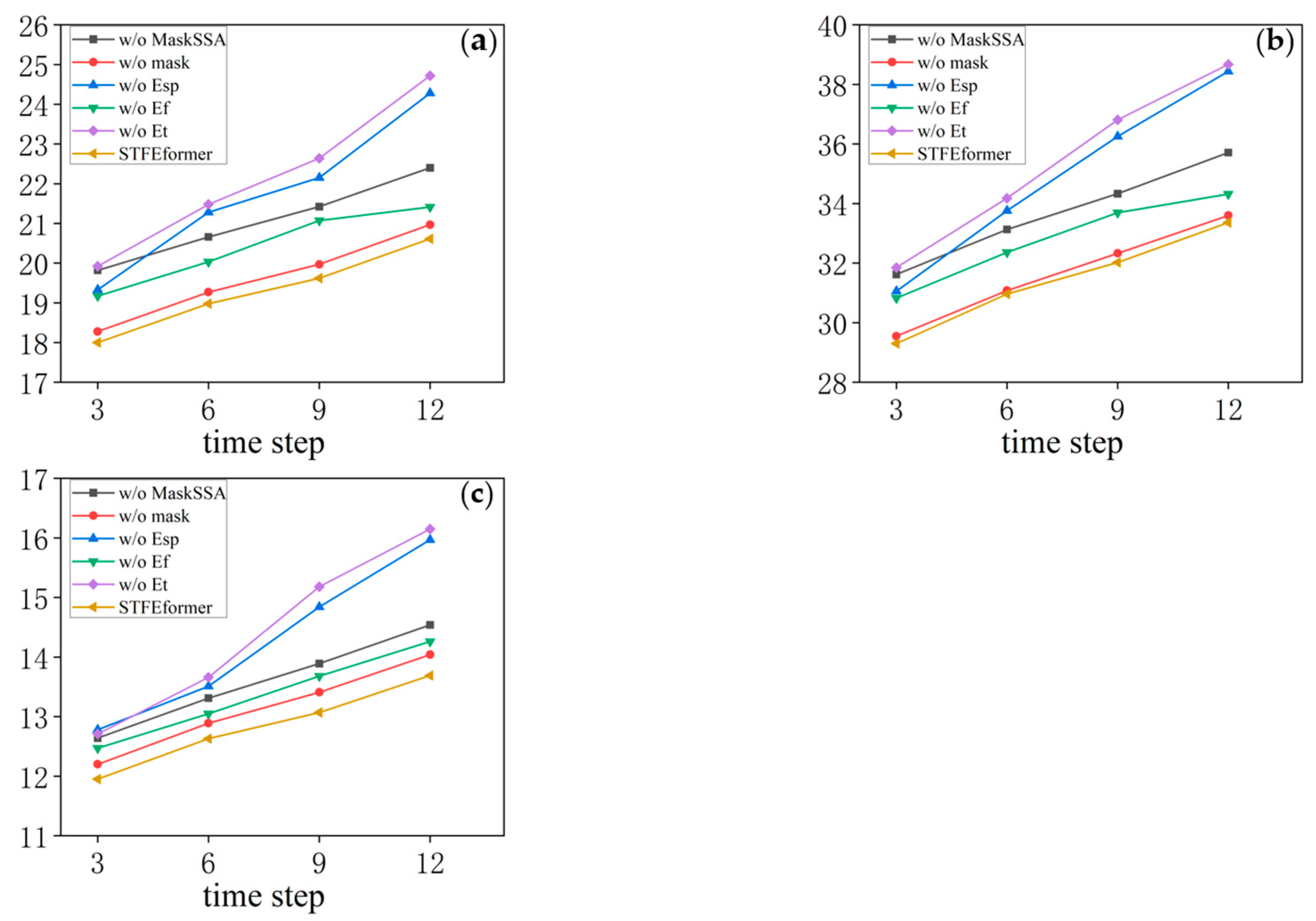
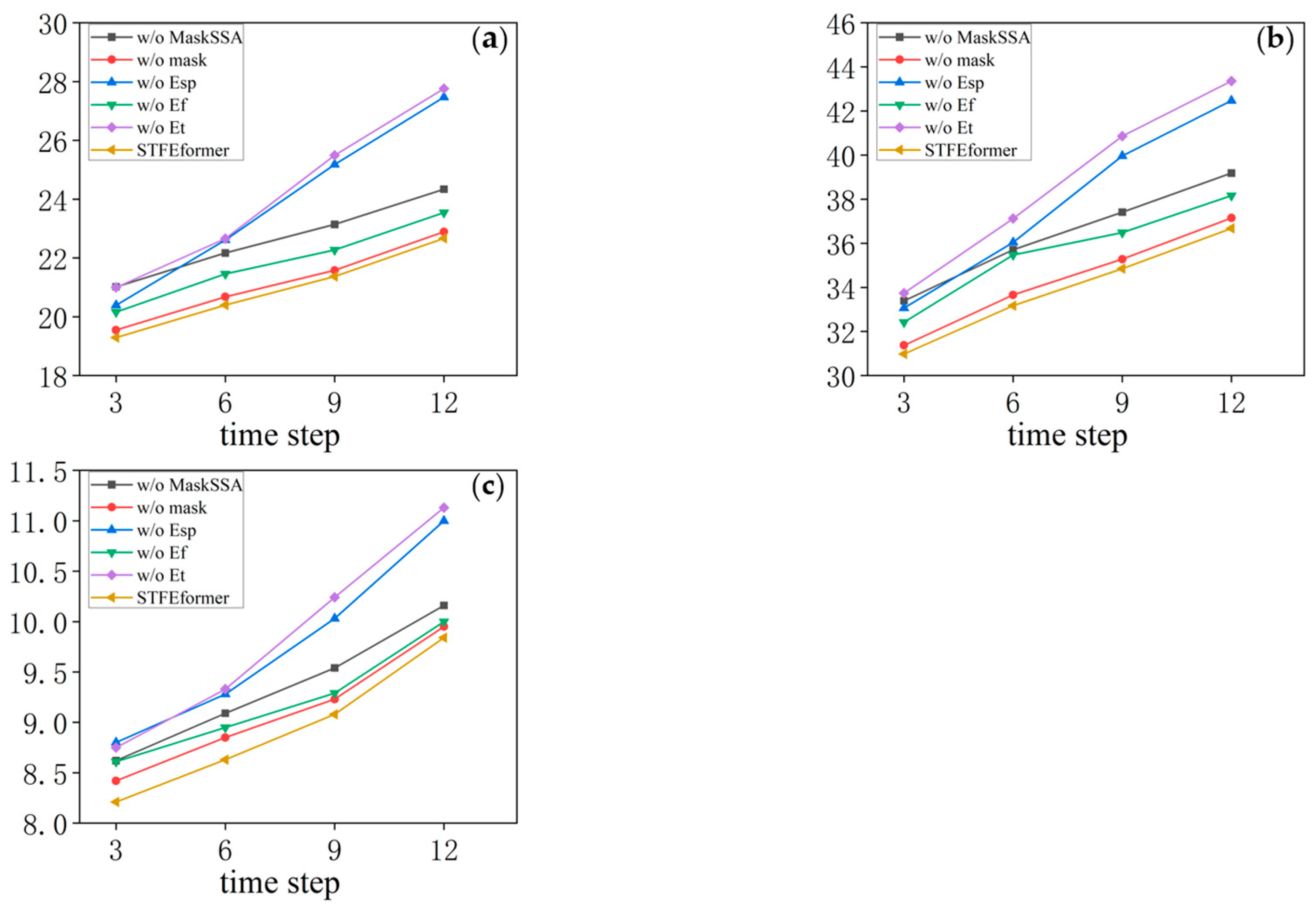
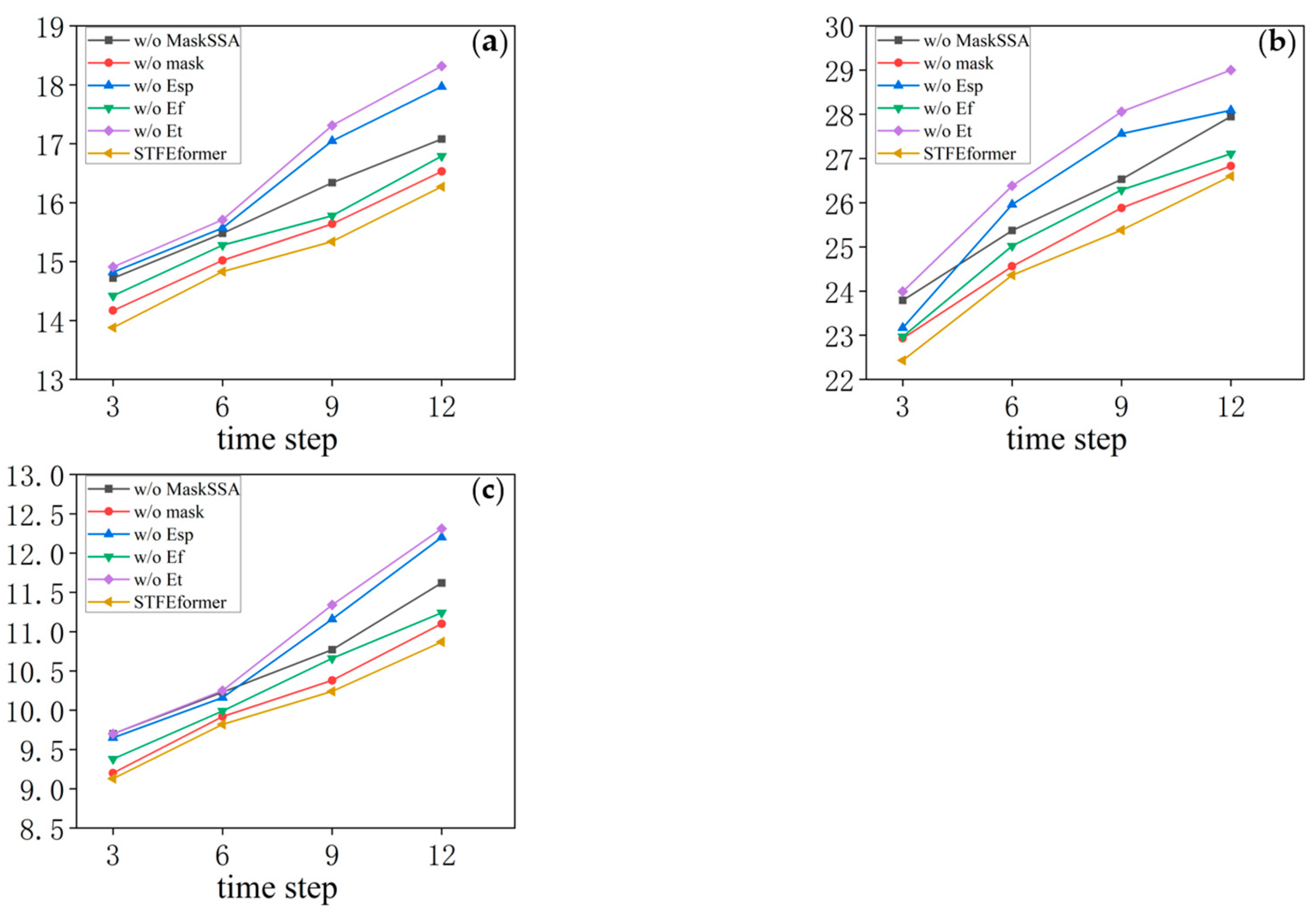
and Figure 2, Figure 3, Figure 4, Figure 5, Figure 6 and Figure 7 illustrating the visualization of the experimental results. The outcomes of the ablation experiments provide a comprehensive perspective on the performance of STFEformer following the removal of different components. Overall, considering 12-time-step prediction, STFEformer performed the best, while w/o $E_t$ ranked the lowest. Compared to the STFEformer model, the performance sequentially decreased for w/o mask, w/o $E_f$, w/o MaskSSA, and w/o $E_{sp}$.

Compared to w/o $E_t$, STFEformer demonstrated a significant improvement in next overall 12-time-step prediction and showed enhancements in MAE, RMSE, and MAPE. For example, STFEformer improved by 13.2%, 11.6%, and 8.0% on the PeMS04 dataset; on the PeMS07 dataset, the improvements were 11.3%, 10.4%, and 7.4%; and on the PeMS08 dataset, the improvements were 7.2%, 8.8%, and 5.7%.

In predicting the next overall 12 time steps, STFEformer achieved enhancements in MAE, RMSE, and MAPE when contrasted with w/o $E_{sp}$. On the PeMS04 dataset, STFEformer demonstrated enhancements of 12.3% in MAE, 10.6% in RMSE, and 7.2% in MAPE. Similarly, on the PeMS07 dataset, the enhancements were 10.6%, 9.2%, and 6.1% in MAE, RMSE, and MAPE, respectively. On the PEMS08 dataset, the enhancements were 5.7%, 7.7%, and 5.1% in MAE, RMSE, and MAPE.

Moreover, in the prediction of the next overall 12 time steps, STFEformer exhibited enhancements on different datasets when contrasted with w/o $E_f$. For instance, the improvements were 5.7%, 4.8%, and 3.5% in MAE, RMSE, and MAPE on the PeMS04 dataset; on the PEMS07 dataset, the improvements were 4.9%, 5.2%, and 3.7; and the improvements were 3.8%, 3.5%, and 3.6% on the PEMS08 dataset, respectively.

Furthermore, compared to w/o mask, STFEformer showed an improvement in next overall 12-time-step prediction. Specifically, on the PeMS04 dataset, STFEformer improved by 1.7%, 1.4%, and 2.5% in MAE, RMSE, and MAPE, respectively. The enhancements were 1.9%, 1.8%, and 1.2% on the PeMS07 dataset, while STFEformer improved by 1.2%, 1.4%, and 2.0% on the PeMS08 dataset.

Finally, compared to w/o MaskSSA, STFEformer showed great improvements. For instance, on the PeMS04 dataset, STFEformer improved by 8.5%, 7.8%, and 5.9%; on the PeMS07 dataset, the improvements were 7.8%, 7.6%, and 4.6%; and on the PeMS08 dataset, STFEformer improved by 4.8%, 4.7%, and 4.5%.

In predictions of the next 15, 30, 45, and 60 min, STFEformer also outperformed all the models post-ablation.

The ablation experiments provide crucial evidence regarding the effectiveness of each component proposed in our research. Through the fusion embedding layer, we successfully achieve comprehensive feature extraction and fusion, significantly enhancing the model’s accuracy for traffic flow prediction tasks. The design of the fusion embedding layer enables the model to extract native information and spatial–temporal characteristics from traffic data more effectively, leading to more accurate prediction. Furthermore, the ablation study underscores the importance of combining an adaptive similarity matrix with spatial self-attention. This method allows the model to concentrate more on the interactions between the similar node pairs during the spatial feature learning process. By accounting for these dynamic and long-range spatial correlations, our model can understand and predict more precisely. Especially when dealing with complex interactions between nodes in urban traffic networks, this mask spatial self-attention mechanism proves particularly crucial.

4.3. Visualization Results

To further validate the effectiveness of STFEformer, we visualized the prediction results for the three datasets and made a comparison between the predicted and target values. The results are shown in Figure 8. It is evident that traffic flow exhibits periodicity, and the prediction results are the same as the target values, demonstrating the model’s success in accurately predicting overall traffic flow trends and capturing these characteristics. Additionally, traffic flow displays distinct short-term features (such as during extreme weather, holidays, or unexpected events) in a certain period of time, and our model also successfully fits these features. Even during periods of dramatic traffic fluctuations, our model accurately captures these changes and closely aligns with actual values. Achieving consistent high performance across different datasets further substantiates the robustness and reliability of our model.

Figure 9 displays the partially adaptive similarity matrices obtained from training on three datasets. In the heat maps of the adaptive similarity matrices, the strength of the similarities between node pairs is markedly evident. Through iteratively training the matrices obtained from the fusion embedding layer across three datasets, similarity matrices that represent the spatial correlations between nodes can be obtained. Figure 9 illustrates the similarity matrices obtained through training for all datasets, revealing a clear aggregation pattern among node pairs with stronger similarities. This observation underscores that STFEformer can effectively symbolize the spatial relationships between different node pairs via the similarity matrices. Therefore, it reiterates the efficacy of the fusion embedding layer in capturing spatial characteristics.

5. Conclusions

In this research, we introduce an STFEformer model designed to improve the understanding of complex traffic data characteristics for traffic flow prediction. Specifically, we introduce a uniquely designed fusion embedding layer to efficiently extract and fuse multi-perspective features, including spatial, temporal (short-term and periodic), and native features in traffic data in order to obtain a more comprehensive representation of traffic data features and lay a solid foundation for accurate traffic flow prediction. We designed a novel spatial self-attention module that leverages a mask matrix method to enhance the detection of dynamic, long-range spatial correlations. To further explore dynamic temporal correlations, a temporal self-attention module is also employed. We conducted extensive experiments to evaluate our model on three real-world public datasets, in which it outperformed twelve baseline models. The ablation experiments, in particular, provide crucial insights into the effectiveness of each component, affirming the significant contribution of our novel mechanisms to the model’s overall performance. Finally, we visualized the prediction results and the learned adaptive similarity matrices, significantly enhancing the interpretability and transparency of our model. These visualizations not only confirm the accuracy of our predictions but also provide intuitive insights into the model’s decision-making process. In the future, we intend to integrate STFEformer with other computational methods such as deep-learning algorithms for real-time data analysis and apply our model to diverse contexts, such as smart city planning and autonomous vehicle navigation, in order to delve deeper into the hidden information in spatial–temporal data and discover the impact of spatial–temporal dimensions on prediction accuracy. By pursuing this way, our objective is to further improve the predictive performance of STFEformer and discover its potential applications in different tasks. Moreover, we will further investigate mechanisms that can dynamically update traffic networks to reflect real-time changes in traffic patterns.

References

1. Yin, C.T.; Xiong, Z.; Chen, H.; Wang, J.Y.; Cooper, D.; David, B. A Literature Survey on Smart Cities. Sci. China Inf. Sci. 2015, 58, 1–18. [Google Scholar] [CrossRef]
2. Tedjopurnomo, D.A.; Bao, Z.F.; Zheng, B.H.; Choudhury, F.; Qin, A.K. A Survey on Modern Deep Neural Network for Traffic Prediction: Trends, Methods and Challenges. IEEE Trans. Knowl. Data Eng. 2022, 34, 1544–1561. [Google Scholar] [CrossRef]
3. Wang, J.; Jiang, J.; Jiang, W.; Li, C.; Zhao, W.X. Libcity: An Open Library for Traffic Prediction. In Proceedings of the 29th International Conference on Advances in Geographic Information Systems, Beijing, China, 2–5 November 2021. [Google Scholar]
4. Yin, X.; Wu, G.; Wei, J.; Shen, Y.; Qi, H.; Yin, B. Deep Learning on Traffic Prediction: Methods, Analysis, and Future Directions. IEEE Trans. Intell. Transp. Syst. 2021, 23, 4927–4943. [Google Scholar] [CrossRef]
5. Yao, H.; Wu, F.; Ke, J.; Tang, X.; Jia, Y.; Lu, S.; Gong, P.; Ye, J.; Li, Z. Deep Multi-View Spatial-Temporal Network for Taxi Demand Prediction. In Proceedings of the AAAI Conference on Artificial Intelligence, New Orleans, LA, USA, 2–7 February 2018. [Google Scholar]
6. Zhang, J.; Zheng, Y.; Qi, D. Deep Spatio-Temporal Residual Networks for Citywide Crowd Flows Prediction. In Proceedings of the AAAI Conference on Artificial Intelligence, San Francisco, CA, USA, 4–9 February 2017. [Google Scholar]
7. Li, Y.; Yu, R.; Shahabi, C.; Liu, Y. Diffusion Convolutional Recurrent Neural Network: Data-Driven Traffic Forecasting. arXiv 2017, arXiv:1707.01926. [Google Scholar]
8. Yu, B.; Yin, H.; Zhu, Z. Spatio-Temporal Graph Convolutional Networks: A Deep Learning Framework for Traffic Forecasting. arXiv 2017, arXiv:1709.04875. [Google Scholar]
9. Bai, L.; Yao, L.; Li, C.; Wang, X.; Wang, C. Adaptive Graph Convolutional Recurrent Network for Traffic Forecasting. Adv. Neural Inf. Process. Syst. 2020, 33, 17804–17815. [Google Scholar]
10. Hu, J.; Lin, X.; Wang, C. Dstgcn: Dynamic Spatial-Temporal Graph Convolutional Network for Traffic Prediction. IEEE Sens. J. 2022, 22, 13116–13124. [Google Scholar] [CrossRef]
11. Wang, J.; Wang, W.; Yu, W.; Liu, X.; Jia, K.; Li, X.; Zhong, M.; Sun, Y.; Xu, Y. Sthgcn: A Spatiotemporal Prediction Framework Based on Higher-Order Graph Convolution Networks. Knowl. Based Syst. 2022, 258, 109985. [Google Scholar] [CrossRef]
12. Yu, H.; Li, T.; Yu, W.; Li, J.; Huang, Y.; Wang, L.; Liu, A. Regularized Graph Structure Learning with Semantic Knowledge for Multi-Variates Time-Series Forecasting. arXiv 2022, arXiv:2210.06126. [Google Scholar]
13. Zhao, J.; Chen, C.; Liao, C.; Huang, H.; Ma, J.; Pu, H.; Luo, J.; Zhu, T.; Wang, S. 2f-Tp: Learning Flexible Spatiotemporal Dependency for Flexible Traffic Prediction. IEEE Trans. Intell. Transp. Systems. 2022, 24, 15379–15391. [Google Scholar] [CrossRef]
14. Zhao, L.; Song, Y.; Zhang, C.; Liu, Y.; Wang, P.; Lin, T.; Deng, M.; Li, H. T-Gcn: A Temporal Graph Convolutional Network for Traffic Prediction. IEEE Trans. Intell. Transp. Syst. 2019, 21, 3848–3858. [Google Scholar] [CrossRef]
15. Wu, Z.; Pan, S.; Long, G.; Jiang, J.; Chang, X.; Zhang, C. Connecting the Dots: Multivariate Time Series Forecasting with Graph Neural Networks. In Proceedings of the 26th ACM SIGKDD International Conference on Knowledge Discovery & Data Mining, San Diego, CA, USA, 23–27 August 2020. [Google Scholar]
16. Cao, S.; Wu, L.; Wu, J.; Wu, D.; Li, Q. A Spatio-Temporal Sequence-to-Sequence Network for Traffic Flow Prediction. Inf. Sci. 2022, 610, 185–203. [Google Scholar] [CrossRef]
17. Li, F.; Yan, H.; Jin, G.; Liu, Y.; Li, Y.; Jin, D. Automated Spatio-Temporal Synchronous Modeling with Multiple Graphs for Traffic Prediction. In Proceedings of the 31st ACM International Conference on Information & Knowledge Management, Atlanta, GA, USA, 17–21 October 2022. [Google Scholar]
18. Sun, Y.; Jiang, X.; Hu, Y.; Duan, F.; Guo, K.; Wang, B.; Gao, J.; Yin, B. Dual Dynamic Spatial-Temporal Graph Convolution Network for Traffic Prediction. IEEE Trans. Intell. Transp. Syst. 2022, 23, 23680–23693. [Google Scholar] [CrossRef]
19. Ta, X.; Liu, Z.; Hu, X.; Yu, L.; Sun, L.; Du, B. Adaptive Spatio-Temporal Graph Neural Network for Traffic Forecasting. Knowl. Based Syst. 2022, 242, 108199. [Google Scholar] [CrossRef]
20. Fang, Z.; Long, Q.; Song, G.; Xie, K. Spatial-Temporal Graph Ode Networks for Traffic Flow Forecasting. In Proceedings of the 27th ACM SIGKDD Conference on Knowledge Discovery & Data Mining, Singapore, 14–18 August 2021. [Google Scholar]
21. Lan, S.; Ma, Y.; Huang, W.; Wang, W.; Yang, H.; Li, P. Dstagnn: Dynamic Spatial-Temporal Aware Graph Neural Network for Traffic Flow Forecasting. In Proceedings of the International Conference on Machine Learning, Guangzhou, China, 18–21 February 2022. [Google Scholar]
22. Li, M.; Zhu, Z. Spatial-Temporal Fusion Graph Neural Networks for Traffic Flow Forecasting. In Proceedings of the AAAI Conference on Artificial Intelligence, Virtually, 2–9 February 2021. [Google Scholar]
23. Song, C.; Lin, Y.; Guo, S.; Wan, H. Spatial-Temporal Synchronous Graph Convolutional Networks: A New Framework for Spatial-Temporal Network Data Forecasting. In Proceedings of the AAAI Conference on Artificial Intelligence, New York, NY, USA, 7–12 February 2020. [Google Scholar]
24. Wu, Z.; Pan, S.; Long, G.; Jiang, J.; Zhang, C. Graph Wavenet for Deep Spatial-Temporal Graph Modeling. arXiv 2019, arXiv:1906.00121. [Google Scholar]
25. Zheng, C.; Fan, X.; Wang, C.; Qi, J. Gman: A Graph Multi-Attention Network for Traffic Prediction. In Proceedings of the AAAI Conference on Artificial Intelligence, New York, NY, USA, 7–12 February 2020. [Google Scholar]
26. Feng, A.; Tassiulas, L. Adaptive Graph Spatial-Temporal Transformer Network for Traffic Forecasting. In Proceedings of the 31st ACM International Conference on Information & Knowledge Management, Atlanta, GA, USA, 17–21 October 2022. [Google Scholar]
27. Cai, L.; Janowicz, K.; Mai, G.; Yan, B.; Zhu, R. Traffic Transformer: Capturing the Continuity and Periodicity of Time Series for Traffic Forecasting. Trans. GIS 2020, 24, 736–755. [Google Scholar] [CrossRef]
28. Chen, Y.; Zheng, L.; Liu, W. Spatio-Temporal Attention-Based Graph Convolution Networks for Traffic Prediction. In Proceedings of the 2022 IEEE International Conference on Systems, Man, and Cybernetics (SMC), Prague, Czech Republic, 9–12 October 2022. [Google Scholar]
29. Fang, Y.; Zhao, F.; Qin, Y.; Luo, H.; Wang, C. Learning All Dynamics: Traffic Forecasting Via Locality-Aware Spatio-Temporal Joint Transformer. IEEE Trans. Intell. Transp. Syst. 2022, 23, 23433–23446. [Google Scholar] [CrossRef]
30. Guo, S.; Lin, Y.; Wan, H.; Li, X.; Cong, G. Learning Dynamics and Heterogeneity of Spatial-Temporal Graph Data for Traffic Forecasting. IEEE Trans. Knowl. Data Eng. 2021, 34, 5415–5428. [Google Scholar] [CrossRef]
31. Li, Y.; Moura, J.M. Forecaster: A Graph Transformer for Forecasting Spatial and Time-Dependent Data. arXiv 2019, arXiv:1909.04019. [Google Scholar]
32. Li, Y.; Wang, H.; Li, J.; Liu, C.; Tan, J. Act: Adversarial Convolutional Transformer for Time Series Forecasting. In Proceedings of the 2022 International Joint Conference on Neural Networks (IJCNN), Padua, Italy, 18–23 July 2022. [Google Scholar]
33. Liu, H.; Dong, Z.; Jiang, R.; Deng, J.; Deng, J.; Chen, Q.; Song, X. Spatio-Temporal Adaptive Embedding Makes Vanilla Transformer Sota for Traffic Forecasting. In Proceedings of the 32nd ACM International Conference on Information and Knowledge Management, Birmingham, UK, 21–25 October 2023. [Google Scholar]
34. Wang, Q.; He, G.; Lu, P.; Chen, Q.; Chen, Y.; Huang, W. Spatial-Temporal Graph-Based Transformer Model for Traffic Flow Forecasting. In Proceedings of the 2022 IEEE 25th International Conference on Intelligent Transportation Systems (ITSC), Macau, China, 8–12 October 2022. [Google Scholar]
35. Yan, H.; Ma, X.; Pu, Z. Learning Dynamic and Hierarchical Traffic Spatiotemporal Features with Transformer. IEEE Trans. Intell. Transp. Syst. 2021, 23, 22386–22399. [Google Scholar] [CrossRef]
36. Ye, X.; Fang, S.; Sun, F.; Zhang, C.; Xiang, S. Meta Graph Transformer: A Novel Framework for Spatial–Temporal Traffic Prediction. Neurocomputing 2022, 491, 544–563. [Google Scholar] [CrossRef]
37. Zhang, H.; Zou, Y.; Yang, X.; Yang, H. A Temporal Fusion Transformer for Short-Term Freeway Traffic Speed Multistep Prediction. Neurocomputing 2022, 500, 329–340. [Google Scholar] [CrossRef]
38. Vaswani, A.; Shazeer, N.; Parmar, N.; Uszkoreit, J.; Jones, L.; Gomez, A.N.; Kaiser, Ł.; Polosukhin, I. Attention Is All You Need. Adv. Neural Inf. Process. Syst. 2017, 30, 5998–6008. [Google Scholar]
39. Zivot, E.; Wang, J. Modeling Financial Time Series with S-PLUS®, 3rd ed.; Springer: New York, NY, USA, 2006; pp. 385–429. [Google Scholar]
40. Drucker, H.; Burges, C.J.; Kaufman, L.; Smola, A.; Vapnik, V. Support Vector Regression Machines. Adv. Neural Inf. Process. Syst. 1996, 9, 155–161. [Google Scholar]
41. Guo, S.; Lin, Y.; Feng, N.; Song, C.; Wan, H. Attention Based Spatial-Temporal Graph Convolutional Networks for Traffic Flow Forecasting. In Proceedings of the AAAI Conference on Artificial Intelligence, Honolulu, HI, USA, 27 January–1 February 2019. [Google Scholar]
42. Chen, Y.; Segovia, I.; Gel, Y.R. Z-Gcnets: Time Zigzags at Graph Convolutional Networks for Time Series Forecasting. In Proceedings of the International Conference on Machine Learning, Virtual, 18–24 July 2021. [Google Scholar]
43. Chen, Y.; Qin, Y.; Li, K.; Yeo, C.K.; Li, K. Adaptive Spatial-Temporal Graph Convolution Networks for Collaborative Local-Global Learning in Traffic Prediction. IEEE Trans. Veh. Technol. 2023, 72, 12653–12663. [Google Scholar] [CrossRef]
Figure 1. The framework of STFEformer.
Applsci 14 04325 g001
Figure 2. The overall 12-time-step prediction results of the ablation study on PeMS04. (a) MAE. (b) RMSE. (c) MAPE.
Applsci 14 04325 g002
Figure 3. The overall 12-time-step prediction results of the ablation study on PeMS07. (a) MAE. (b) RMSE. (c) MAPE.
Applsci 14 04325 g003
Figure 4. The overall 12-time-step prediction results of the ablation study on PeMS08. (a) MAE. (b) RMSE. (c) MAPE.
Applsci 14 04325 g004
Figure 5. The next 3-, 6-, 9-, and 12-time-step prediction results of the ablation study on PeMS04. (a) MAE. (b) RMSE. (c) MAPE.
Applsci 14 04325 g005
Figure 6. The next 3-, 6-, 9-, and 12-time-step prediction results of the ablation study on PeMS07. (a) MAE. (b) RMSE. (c) MAPE.
Applsci 14 04325 g006
Figure 7. The next 3-, 6-, 9-, and 12-time-step prediction results of the ablation study on PeMS08. (a) MAE. (b) RMSE. (c) MAPE.
Applsci 14 04325 g007
Figure 8. The visualization results for prediction. (a) PeMS04. (b) PeMS07. (c) PeMS08.
Applsci 14 04325 g008
Figure 9. Heat maps of the similarity matrix for (a) PeMS04, (b) PeMS07, and (c) PeMS08.
Applsci 14 04325 g009