Study of Tunnel Vehicle GNSS/INS/OD Combination Position Based on Lateral Distance Measurement and Lane Line Constraint

Abstract

The high-precision dynamic positioning of highway vehicles is the foundation and prerequisite for achieving intelligent connected transportation. To address the shortcomings of the GNSS/INS combination and GNSS/INS/OD combination in tunnel vehicle positioning, this paper proposes a tunnel vehicle positioning method for the GNSS/INS/OD combination based on lateral distance measurements and lane constraints. Firstly, a lateral distance measurement of vehicles inside the tunnel is conducted based on laser radar point cloud data. Secondly, map matching positioning is performed based on lateral distance measurements, odometer, and lane markings. Experimental results demonstrate that, for a 4.6 km tunnel, the average absolute error in the lateral positioning is 0.294 m, and the longitudinal positioning error is no more than 0.6 m, which can effectively meet practical operational requirements.

1. Introduction

Currently, many countries are vigorously developing intelligent, connected, vehicle–road cooperative technologies [1]. Intelligent connected vehicles have become a strategic direction for the development of the global automotive industry [2]. The high-precision dynamic positioning of highway vehicles serves as the foundation and a prerequisite for achieving intelligent connected transportation [3]. A high-precision spatio-temporal reference service is listed as the key basic technology that needs to be established [4], and the high-precision intelligent navigation of unmanned vehicles under the condition that satellites are not available is listed as one of the ten major engineering and technical problems [5].

There are two main methods for vehicle mobile positioning: satellite navigation and inertial navigation [6]. As long as a Global Navigation Satellite System (GNSS) can receive the navigation satellite signal, it can calculate the position and speed of the vehicle [7]. An Inertial Navigation System (INS) works based on the inertial principle and does not need any external information when working, but navigation errors accumulate over time [8].

In general road environments, a GNSS can be applied to achieve vehicle positioning [9]. In short-range shielded environments, vehicles can maintain a good continuous positioning performance based on a combination of a GNSS and INS [10,11,12]. However, in strongly shielded environments, such as long tunnels, effectively suppressing the divergence speed of the INS is an important issue that urgently needs to be addressed [13,14]. When GNSS signals are unavailable because of obstruction, multipath effects, etc., the GNSS/INS/odometer (OD) combination can effectively mitigate the accumulation of INS errors to a certain extent, achieving the high-precision stable navigation and positioning of the vehicle [15,16].

To simulate the positioning performance of tunnel vehicles using a GNSS/INS/OD combination, the authors conducted experiments on a certain section of the highway where all GNSS signals were artificially removed. Only inertial navigation and the odometer were used for dead reckoning, and the GNSS/INS data fusion results were used as the reference trajectory (truth value) for comparison. The experimental results indicate that as the dead reckoning distance increases, the positioning results deviate more and more from the true trajectory. At a distance of 545 m, the positioning error is approximately 0.88 m [17]. This cannot meet the practical requirements for tunnel vehicle positioning.

The reason for this lies in the fact that, during vehicle motion, the output of inertial devices contains significant noise. How to distinguish between valid data and noise and reduce the impact of vibration noise on system stability and positioning accuracy remains to be studied [18,19,20]. In different scenarios, when the effectiveness of sensors in the integrated navigation system changes, corresponding adjustments need to be made to the state space model [21,22]. Multi-sensor systems are often heterogeneous due to their different principles, making it a challenge to construct reliable multi-sensor fusion function models that can accommodate the real-time addition and removal of sensor types [23,24].

Based on this, this paper uses high-precision digital lane maps, as well as the advantages of LiDAR in distance measurement and odometry in mileage counting, to propose a combined GNSS/INS/OD positioning method for tunnel vehicles based on lateral distance measurement and lane line constraints. It mainly consists of two steps: (1) the lateral distance measurement of vehicles inside a tunnel based on laser radar point cloud data; (2) map matching combined positioning based on lateral distance measurements, odometer, and lane markings. The prerequisite for this positioning method is that a high-precision electronic map of the tunnel has previously been measured or obtained.

2. Research on Lateral Distance Measurements for Tunnel Vehicle Localization

The principle of a laser radar, also known as Light Detection and Ranging (LiDAR), is based on its emitting an infrared laser beam from the radar itself and receiving the reflected infrared beam from the surrounding environment. By measuring the time between the emission and reception of the laser pulses, the distance can be calculated. Taking the example of a VLP-16 LiDAR (Figure 1), this consists of 16 laser beams distributed within a 30° angle. The beams are evenly spaced at a 2° interval, with 15° covering the upward and downward directions.

Using LiDAR to obtain lateral distance measurements of tunnel vehicles, the specific method is as follows:

(1)

Classify LiDAR points into surface feature points and line feature points based on curvature, and remove the line feature points.

By applying the LiDAR-measured point cloud data of the tunnel, calculate the curvature of each point using the following formula:

$$c=\frac{1}{\left|S\right|·‖X_{\left(k,i\right)}^L‖}‖\sum _{jϵS,j\ne i}\left({X_{\left(k,j\right)}^L-X}_{\left(k,i\right)}^L\right)‖$$

(1)

In the equation, $S$ represents the set of five continuous points obtained by the same laser beam; $X_{\left(k,j\right)}^L$ and $X_{\left(k,i\right)}^L$ represent the coordinates of the j-th and i-th points in the k-th frame in the LiDAR coordinate system. Typically, the points with the highest curvature are selected as line feature points, while those with the lowest curvature are considered surface feature points.

(2)

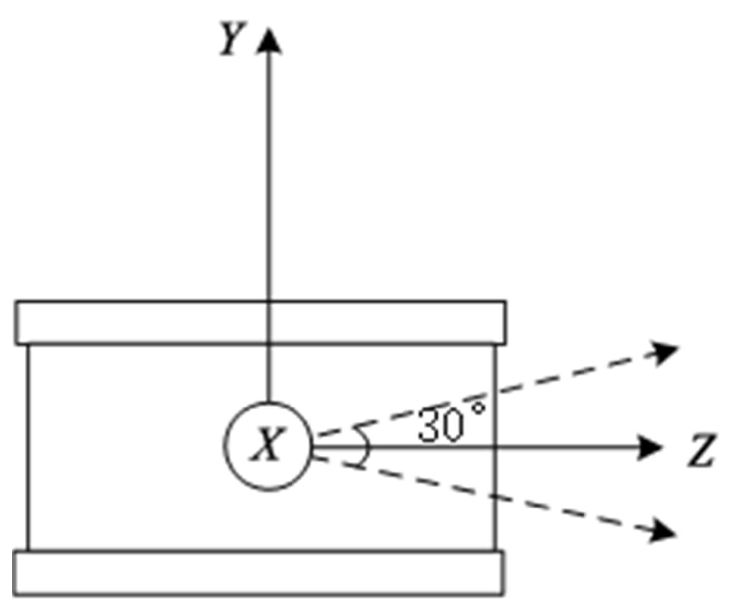
Calculate the horizontal distance from the LiDAR to obstacles when LiDAR is horizontal and select the m smallest values. These values correspond to the point cloud data that form a set $\left\{D\right\}$.

Assuming the maximum elevation angle of the LiDAR is $\theta$, select the point cloud data with an elevation angle of $\theta$ obtained from step (1). Calculate the horizontal distance between the LiDAR and obstacles at different horizontal rotation angles when the elevation angle is $\theta$, using the following formula:

$$d^{\gamma }=l_{\theta }·\cos \theta$$

(2)

$${\left\{D\right\}}_m, d_D^{\gamma }=\min d^{\gamma }$$

(3)

In the equation, $\gamma$ represents the horizontal rotation angle of the LiDAR, $d^{\gamma }$ represents the horizontal distance between the LiDAR and obstacles at an elevation angle of $\theta$ and a horizontal rotation angle of $\gamma$, and $l_{\theta }$ represents the slope distance between the LiDAR and obstacles at an elevation angle of $\theta$ and a horizontal rotation angle of $\gamma$. $\left\{D\right\}$ represents the set of point cloud data from the m LiDARs with the smallest $d^{\gamma }$, and m represents the length of $\left\{D\right\}$. Refer to Figure 2 for illustration.

(3)

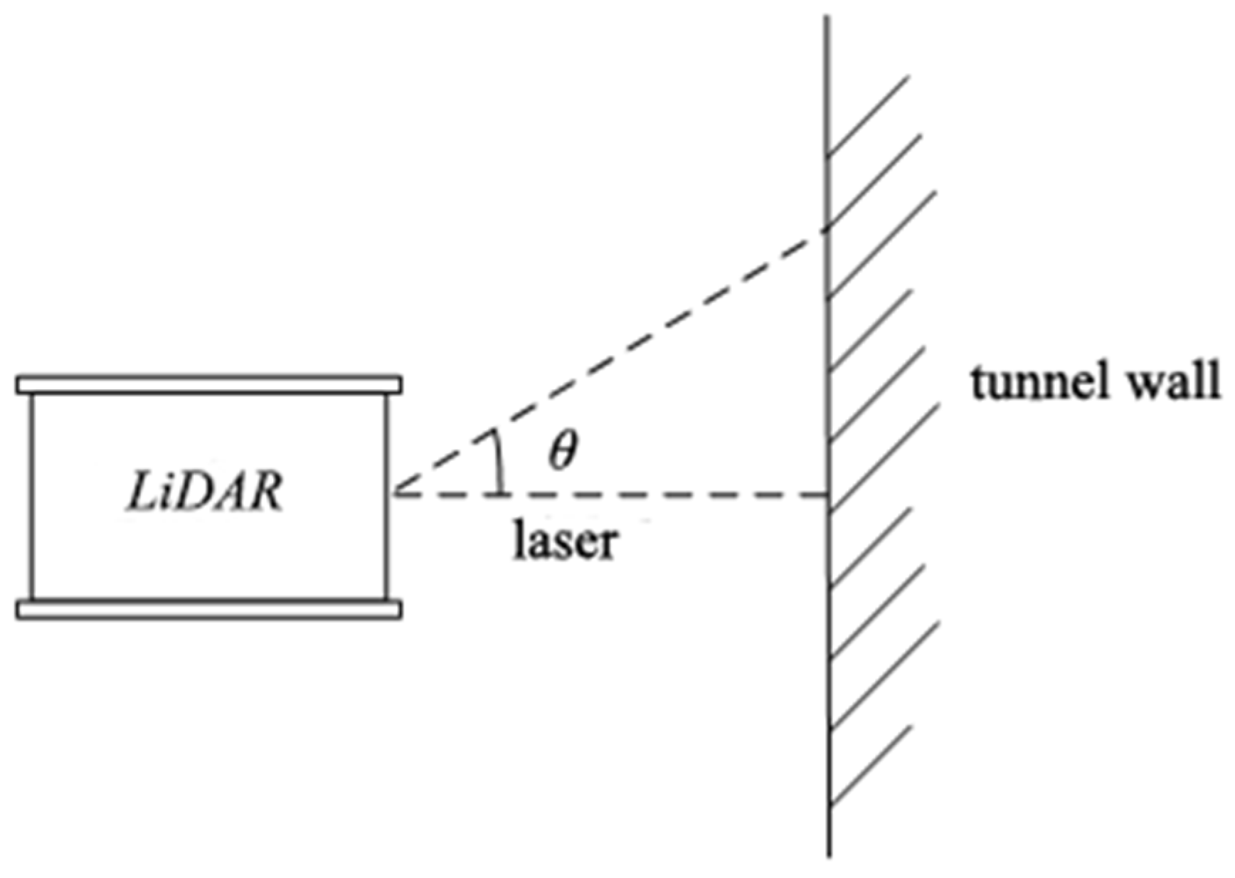
Calculate the horizontal distance from the LiDAR to obstacles when it is tilted.

Uneven road surfaces or the tilting of the LiDAR may cause it to be non-horizontal, as shown in Figure 3.

Select the point cloud data obtained from the LiDAR with an elevation angle of $\alpha (\alpha <\theta )$ from step (1). For each LiDAR point in $\left\{D\right\}$ described in step (2), select the point cloud data with the same horizontal rotation angle and an elevation angle of $\alpha$, then calculate the horizontal distance $d^l$ between the LiDAR and obstacles at that horizontal rotation angle. The calculation formula is as follows:

$$a=\sqrt{l_{\theta }^2+l_{\alpha }^2-2l_{\theta }{l}_{\alpha }\cos \left(\theta -\alpha \right)}$$

(4)

$$d^l=l_{\theta }·\sqrt{1-{\left(\frac{a^2+l_{\theta }^2-l_{\alpha }^2}{2a{l}_{\theta }}\right)}^2}$$

(5)

In the equation, $\alpha$ represents the elevation angle of the LiDAR, where $\alpha <\theta$. $a$ represents the distance between a LiDAR point with an elevation angle of $\theta$ and a horizontal rotation angle of $\gamma$ and another LiDAR point with an elevation angle of $\alpha$ and a horizontal rotation angle of $\gamma$.$l_{\alpha }$ represents the slope distance between the LiDAR and obstacles measured at an elevation angle of $\alpha$ and a horizontal rotation angle of $\gamma$. $d^l$ represents the horizontal distance between the LiDAR and obstacles measured at a horizontal rotation angle $\gamma$.

(4)

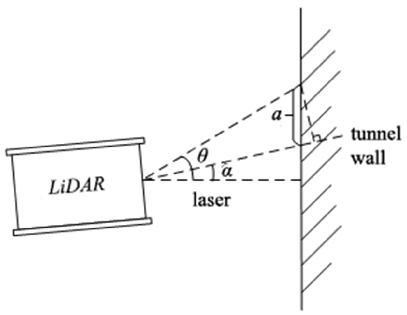
Calculate the precise horizontal distance between the LiDAR and obstacles.

Based on parameter $d^l$ described in step (3), use the following formula:

$$d=\min d^l$$

(6)

In the equation, $d$ represents the precise distance value between the LiDAR and obstacles, where is the minimum value among $d^l$.

(5)

Calculate the distance from the LiDAR to the other side of the obstacles.

Select the distances $l_{\theta 1}$ measured between the LiDAR and obstacles at an elevation angle of $\theta$ and a horizontal rotation angle of $\phi +\pi$ from step (1), as well as the distances $l_{\alpha 1}$ measured at an elevation angle of $\alpha (\alpha <\theta )$ and a horizontal rotation angle of $\phi +\pi$. Calculate the distance between the LiDAR and obstacles on the other side using the following formula:

$$a^{\prime }=\sqrt{l_{\theta 1}^2+l_{\alpha 1}^2-2l_{\theta 1}{l}_{\alpha 1}\cos \left(\theta -\alpha \right)}$$

(7)

$${d^l}^{\prime }=l_{\theta 1}·\sqrt{1-{\left(\frac{{a^{\prime }}^2+l_{\theta 1}^2-l_{\alpha 1}^2}{2a^{\prime }{l}_{\theta 1}}\right)}^2}$$

(8)

In the equation, $a^{\prime }$ represents the distance between the LiDAR point with an elevation angle of $\theta$ and a horizontal rotation angle of $\phi +\pi$ and the LiDAR point with an elevation angle of $\alpha$ and a horizontal rotation angle of $\phi +\pi$, and ${d^l}^{\prime }$ represents the horizontal distance between the LiDAR and obstacles measured at a horizontal rotation angle $\phi +\pi$.

(6)

Correction of lateral distance.

In tunnels, emergency stopping zones are provided at regular intervals. Additionally, there are situations where large and high vehicles run parallel to the test vehicle. As shown in Figure 4, under these two special circumstances, the calculated lateral distance values are wrong and require correction. Let $\mathrm{d}l$ and $\mathrm{d}r$ represent the horizontal distances from the onboard LiDAR to the left and right obstacles, respectively, and $\mathrm{d}b$ represents the typical width of a tunnel segment. In normal conditions, horizontal distances of the previous time $p$ from the LiDAR to the left and right obstacles are represented by ${\mathrm{d}l}_p$ and ${\mathrm{d}r}_p$, respectively. Considering that the width of the typical tunnel segment remains unchanged, the correction method for the lateral distance is as follows:

$$\left\{\begin{array}{c}\mathrm{d}l=\mathrm{d}l,\mathrm{d}r=\mathrm{d}r \mathrm{d}l+\mathrm{d}r=\mathrm{d}b\\ \mathrm{d}l=\mathrm{d}l,\mathrm{d}r=\mathrm{d}b-\mathrm{d}l \mathrm{d}l+\mathrm{d}r\ne \mathrm{d}b, \mathrm{d}l={\mathrm{d}l}_p,\mathrm{d}r\ne {\mathrm{d}r}_p\\ \mathrm{d}r=\mathrm{d}r,\mathrm{d}l=\mathrm{d}b-\mathrm{d}r \mathrm{d}l+\mathrm{d}r\ne \mathrm{d}b,\mathrm{d}r={\mathrm{d}r}_p, \mathrm{d}l\ne {\mathrm{d}l}_p\\ \mathrm{delete} \mathrm{d}l+\mathrm{d}r\ne \mathrm{d}b, \mathrm{d}l\ne {\mathrm{d}l}_p,\mathrm{d}r\ne {\mathrm{d}r}_p\end{array}\right.$$

(9)

In the equation, within the judgment condition, an error threshold $\delta$ can be added, for example, by setting $\delta =5~10 \mathrm{c}\mathrm{m}$.

3. Combined Positioning of Tunnel Vehicles Constrained by Lane Lines and Lateral Distance

(1)

Determine the starting point of the mileage constraint. Before entering the tunnel, according to the GNSS Real-Time Kinematic (RTK) positioning results of the satellite, the corresponding lane line points are geometrically matched in the vertical direction and are recorded as the starting point of the mileage constraint.

(2)

Calculate accumulated vehicle mileage. According to the wheel speedometer, the cumulative calculation of vehicle mileage is accumulated by the encoder pulse count of the cumulative mileage meter. Assuming that the cumulative number of pulses of the odometer at a certain time is n, the total cumulative mileage at this time is as follows:

$$S=n\times l\times (1+\gamma )$$

(10)

where $l$ denotes the circumference of the wheel (prior value, unit: m), and $\gamma$ represents the perimeter error coefficient in the process of vehicle travel, which is estimated via real-time joint solution calculation with GNSS RTK/INS.

(3)

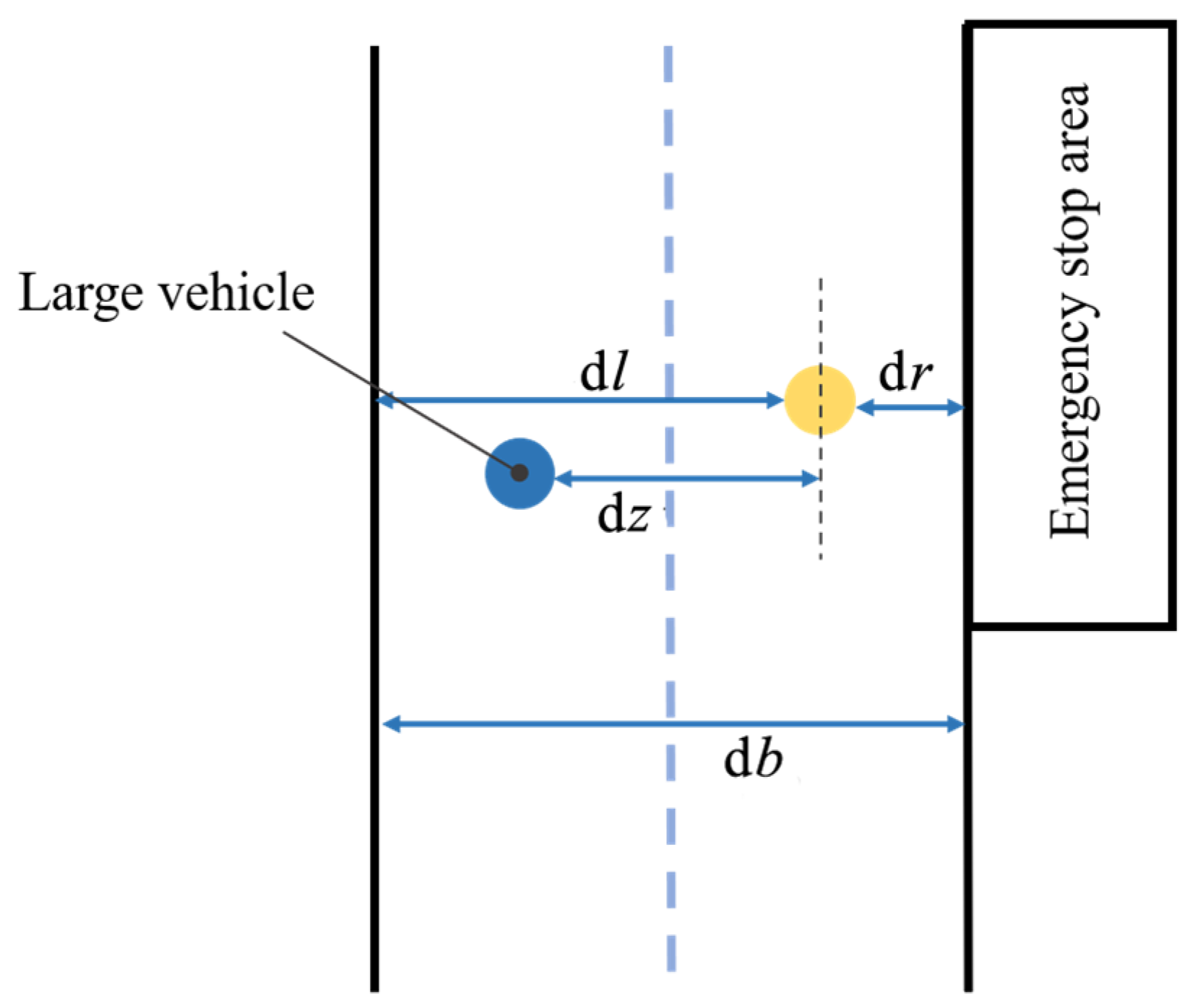
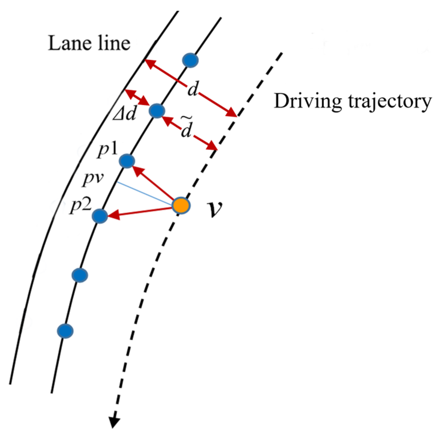
Calculate the distance between the vehicle and the lane line. In the tunnel, assuming that the distance between the lane line and the tunnel wall remains unchanged (there will be a small change in reality), this is $\Delta d$, as shown in Figure 5. The distance between the vehicle and the lane line can be obtained as follows:

$$\tilde{d}=d-\Delta d$$

(11)

(4)

Determine the matching points. As shown in Figure 5, the method of matching the corresponding points of lane lines according to the total mileage $S$ is as follows:

$$\left\{\begin{array}{c}p1=S/b+p_0\\ p2=S/b+p_0+1\end{array}\right.$$

(12)

where $p1$ indicates the previous recent spot number of the match and $p2$ indicates the nearest point of the latter match; $b$ indicates the distance between lane line points (the value in this paper is fixed at 1 m) and $p_0$ indicates the start dot number.

(5)

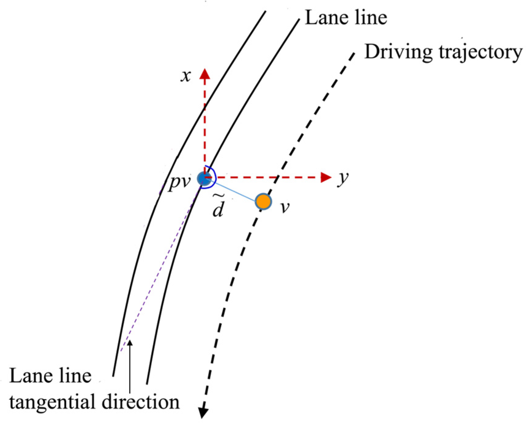
Calculate the coordinates of vertical points. According to the principle of distance division, the coordinates of vertical point $pv$ can be obtained as follows:

$$\left\{\begin{array}{c}{x}_{pv}=x_{p1}+\beta \cdot (x_{p2}-x_{p1})\\ y_{pv}=y_{p1}+\beta \cdot (y_{p2}-y_{p1})\end{array}\right.$$

(13)

where $\beta =S-floor\left(S\right)$,$floor(\cdot )$ indicates the hole down.

(6)

According to the lateral distance of the vehicle from the lane line and the azimuth of the point tangent line, the coordinates of the vehicle point $v$ ($x_v,y_v$) are obtained, as shown in Figure 6 and Formula (14).

$$\left\{\begin{array}{c}{x}_v=x_{pv}-\tilde{d}\cdot \sin (360-\alpha )\\ y_v=y_{pv}-\tilde{d}\cdot \cos (360-\alpha )\end{array}\right.$$

(14)

According to the above mileage matching and lane line constraint positioning method, a higher lateral positioning accuracy can be obtained. However, in the longitudinal direction, due to odometer calibration errors, it is easy to produce mileage accumulation errors when driving for a long time, so in long-distance applications, it is necessary to fully consider the impact of odometer calibration errors. Therefore, this paper proposes a potential positioning for further location combinations of mileage matching positioning results and INS/OD. In other words, the above positioning results are further integrated with the INS/OD combination, and the mileage matching positioning results are used to correct and feedback the INS zero bias errors and odometer scale errors. The odometer calibration error feedback calculated by the INS/OD combination corrects the matching positions of the odometer and lane line, and realizes the mutual correction and complementary advantages of sensors and different positioning means.

4. Case Study of Lateral Distance Measurement

4.1. Static Testing

During the static test, the situation in the tunnel is simulated, the experimental environment is set in the corridor, the LiDAR is placed on the horizontal ground, the algorithm result value is measured by LiDAR, and the results are measured by steel tape. The experimental results of multiple measurements are shown in

Table 1. Test of lateral distance measurements.

Test Number	1		2		3
	Left	Right	Left	Right	Left	Right
Algorithm results/m	0.697	1.301	1.193	0.801	1.565	0.435
Measured results/m	0.710	1.315	1.197	0.821	1.575	0.450
Error/m	0.013	0.014	0.004	0.020	0.010	0.015

. As can be seen from the table, in these measurements, the results of the algorithm have centimeter-level accuracy, the fluctuation range is within 1 cm, and lateral positioning results with centimeter-level accuracy in the tunnel can be obtained.

4.2. Dynamic Test

In a tunnel section, a vehicle lateral location measurement experiment was carried out, and the dynamics and practicability of the algorithm were verified by the actual data. The vehicle drove in the left lane, and the test found that the distance of the vehicle from the left wall was about 5.74 m, the distance from the right wall was about 6.21 m, and the total width of the tunnel was about 11.96 m. According to experience, the design width of the tunnel is about 12 m, so the accuracy of the distance measured from the LiDAR to the walls on both sides of the tunnel meets the requirements. The distance between the vehicle and the walls on both sides cannot remain unchanged during the process of driving, so the distance between the vehicle and the walls on both sides fluctuates within a certain range. At the same time, the measured tunnel width is relatively stable, and the fluctuations are also in the centimeter-level range.

5. Case Study of Combined Positioning in Tunnels

The positioning performance in a real tunnel environment was verified by field tests in the Yudushan Tunnel in Beijing. The tunnel has a total length of 9.2 km, with open sections at the entrances and exits that can receive GNSS signals; however, the interior of the tunnel is a closed environment where GNSS data cannot be received. Vehicles travel at a speed of approximately 60 km/h inside the tunnel. The sensors used for the tests include GNSS RTK, INS, odometer, a laser radar for lateral distance measurements inside the tunnel, and lane map data. GNSS RTK differential data were gotten according to the virtual reference station data provided by Qianxun Location FindCM service.

The tests involved driving from Beijing towards Zhangjiakou (designated as the forward direction), then returning in the opposite direction, making a total of two round trips with four passages through the tunnel. Three methods were used in each test: ① GNSS/INS combination; ② GNSS/INS/OD combination; ③ GNSS/INS/OD combination with lateral distance measurement and lane constraints.

5.1. Comparison of Three Positioning Methods

Figure 7 shows the positioning trajectories of three positioning methods in the tunnel. The green points represent the GNSS/INS combined positioning results, the yellow points represent the GNSS/INS/OD combined positioning results, the red points represent the GNSS/INS/OD combined positioning results constrained by lateral distance and lane lines, and the blue points represent the actual lane lines. From the figure, it can be seen that the GNSS/INS combination deviates the most from the lane lines, with the largest positioning error. The GNSS/INS/OD combination follows; although it shows significant improvements compared to the GNSS/INS combination, the positioning deviation is still considerable over long distances. The GNSS/INS/OD combination with lateral distance lane line constraints provides the best positioning results.

Due to the moving status of vehicles in the tunnel and the lack of means for high-precision dynamic positioning assessment on the roadside, it is difficult to quantitatively evaluate the absolute positioning accuracy in the tunnel. Therefore, in this study, in the open area outside the tunnel, the positioning data were compared with the RTK positioning results obtained at the same time as the first fixed solution to calculate the positioning accuracy when the vehicle exits the tunnel. Figure 8, Figure 9 and Figure 10 show the first positioning results outside the tunnel in the opposite direction. The yellow points represent the first fixed RTK results outside the tunnel, which serve as a reference due to the centimeter-level accuracy of RTK’s fixed solutions; the red points represent the positioning points that are extended from the tunnel positioning method (excluding the GNSS signals received when exiting the tunnel). The distances between corresponding points (at the same time) in the figures represent the errors between the tunnel positioning points and the RTK reference points.

Table 2. Comparison of the horizontal accuracy between the tunnel positioning points and the first fixed RTK point outside the tunnel (unit: m).

Positioning Method	Reverse 1	Reverse 2
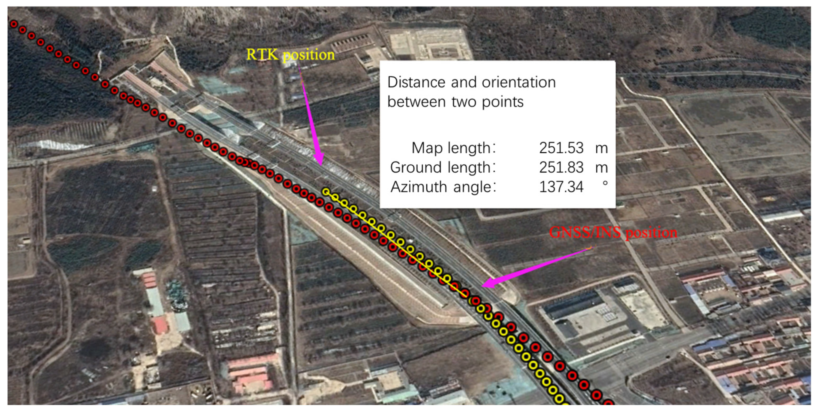
GNSS/INS	251.53	454.55
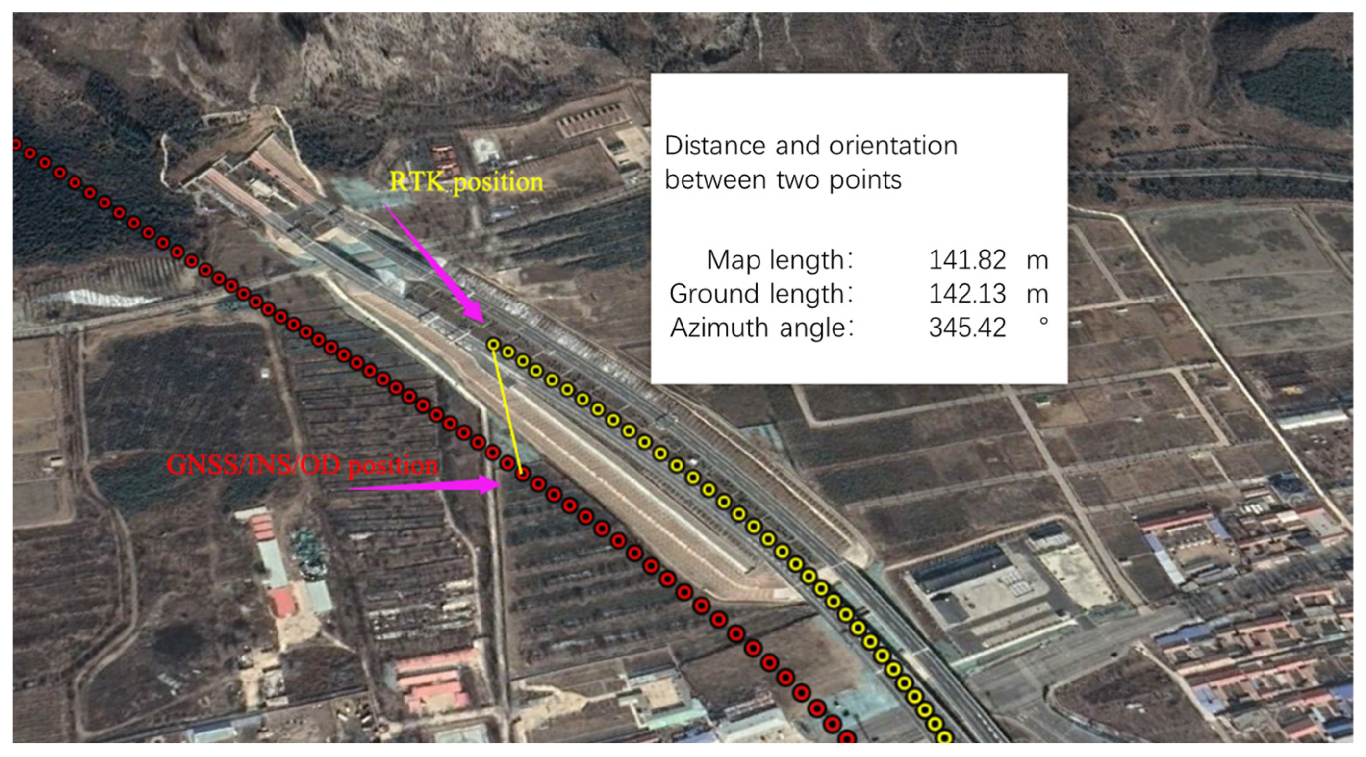
GNSS/INS/OD	141.82	329.78
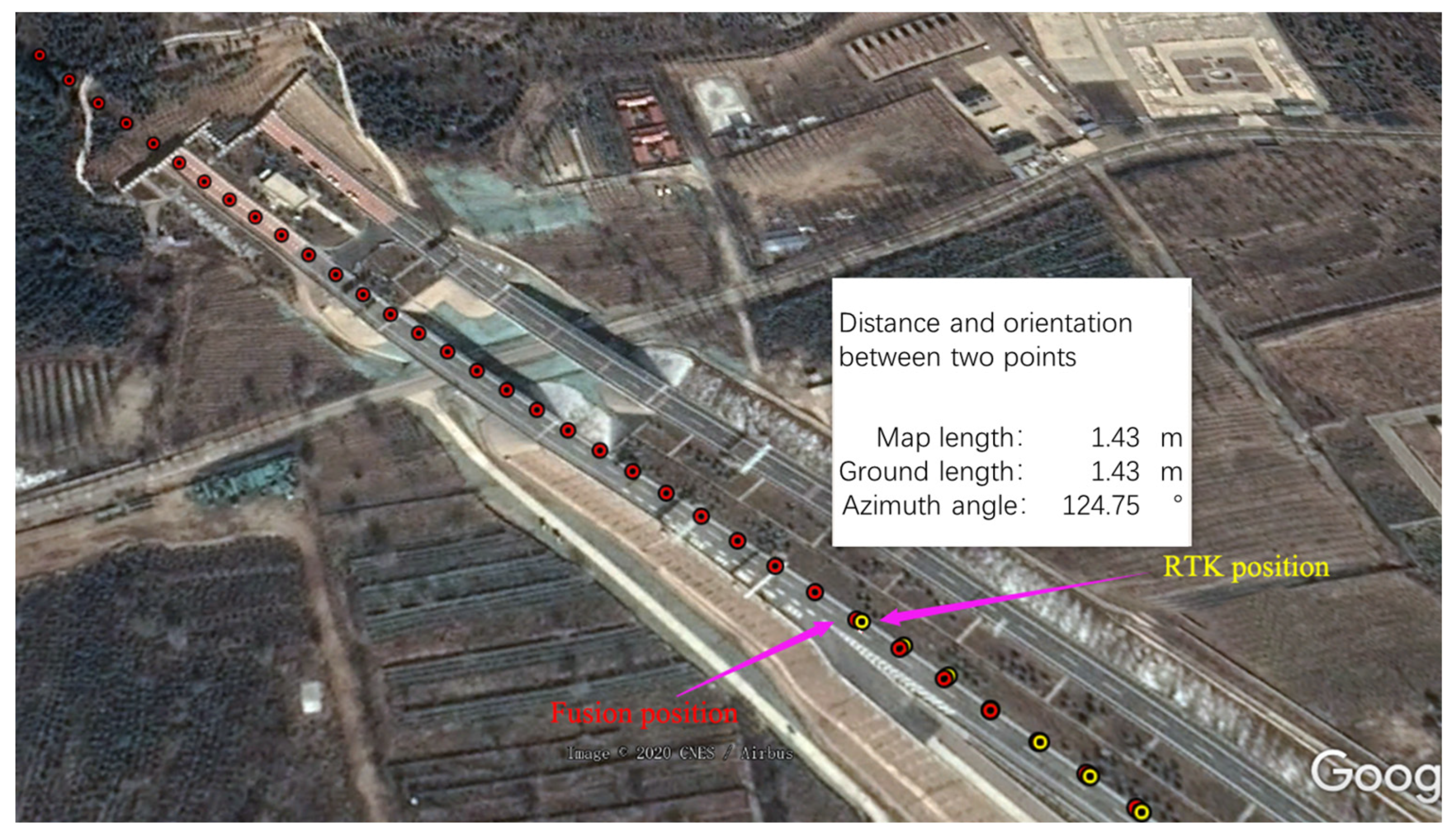
Lateral Distance Measurement + Lane Markings + GNSS/INS/OD	1.43	1.23

provides the corresponding error statistics for two tunnel driving scenarios. It can be seen from the table that in the two sets of experiments, the positioning errors of GNSS/INS and GNSS/INS/OD combinations at the RTK fixed points outside the tunnel are over 100 m, indicating that relying solely on INS, odometers, and other dead reckoning sensors in severe GNSS-denied environments in long tunnels makes it difficult to maintain high-precision positioning and navigation capabilities. The GNSS/INS/OD combination with lateral distance and lane markings constraints provides positioning results that are closest to the RTK results, with a horizontal positioning accuracy between 1.2 m and 1.5 m.

5.2. Analysis of Lateral Positioning Error

In order to quantitatively analyze the lateral accuracy of GNSS/INS/OD combined positioning constrained by lane lines inside the tunnel, the experimental results in the opposite direction are analyzed and statistically processed below. In this experiment, the vehicle’s driving speed inside the tunnel was approximately 60 km/h, as shown in Figure 11. Figure 12 provides the lateral error of a 9.2 km tunnel, with the elliptical marked portion representing a 4.6 km half-length tunnel. The method used to calculate lateral error is as follows: at each comparison moment, calculate the vertical distance between the positioning point and the lane line, then subtract the actual distance of the vehicle from the lane line at the corresponding moment (this distance is obtained by subtracting the lane line distance from the tunnel wall distance measured by LiDAR).

As can be seen from Figure 12, with the increase in driving distance in the tunnel, the positioning error shows a gradually diverging trend. In the second half of the tunnel, the positioning error diverges severely, reaching a maximum of 1 m. The positioning error results for the 4.6 km midpoint of the tunnel are summarized in

Table 3. Statistical analysis of lateral positioning errors in a 4.6 km midpoint tunnel.

Statistical Items	Numerical Value
Number of data points (200 Hz)	61,001
Arithmetic mean of errors	0.013 m
Mean absolute error	0.294 m
Root mean square error	0.332 m
Maximum error value	0.671 m
Minimum error value	−0.865 m
95th percentile of absolute error	0.612 m

. The table includes the arithmetic mean, absolute error mean, root mean square error, maximum error, minimum error, and the 95th percentile of the absolute error. In Table 3, a total of 61,001 positioning points were analyzed. It can be observed that the arithmetic mean of the lateral error is 0.013 m, and the absolute error mean is 0.294 m, which characterizes the absolute lateral accuracy of vehicle positioning. The maximum error and minimum error are 0.671 m and −0.865 m, respectively, with the 95th percentile of the absolute error being 0.612 m, indicating that further improvement is needed in the stability of vehicle positioning in the tunnel.

5.3. Analysis of Longitudinal Positioning Errors

For the longitudinal positioning errors inside the tunnel, due to the lack of reference points for dynamic positioning evaluation within the tunnel, the longitudinal accuracy at the 9.2 km tunnel entrance based on RTK positioning results is used to infer the longitudinal accuracy over the 4.6 km tunnel length. Similarly, an analysis was conducted using the experimental results in the reverse direction. When the vehicle first obtains a fixed RTK solution upon exiting the tunnel, a comparison between the positioning points extended via the tunnel’s positioning method and the RTK positioning points is shown in Figure 10. At this point, the total horizontal positioning error is 1.43 m, and after subtracting the lateral positioning error of that point (0.86 m), the longitudinal positioning error is calculated to be 1.14 m. Based on the divergence characteristics of INS based on navigation estimation sensors and the cumulative nature of odometer errors with distance, it is known that the positioning error diverges faster with increasing driving distance, and the divergence speed in the latter half of the journey is significantly faster than that in the first half, as indicated in Figure 12, which also shows a similar phenomenon in the lateral positioning results. Therefore, it can be conservatively estimated that the longitudinal positioning error at the 4.6 km mark of the tunnel is no greater than 0.6 m. It should be noted that this longitudinal error is only an inferred value based on the results at the tunnel exit, representing a general accuracy level. The positioning errors at different positions within the tunnel may still fluctuate due to various measurement errors, as illustrated in Figure 12.

6. Conclusions

Building upon the GNSS/INS/OD combination positioning, this paper proposes a lane-constrained positioning method integrating odometer mileage calculation and laser radar lateral distance measurements. The constrained positioning results are used to update the measurements, achieving fusion between lane-constrained positioning within the tunnel and INS/OD combination positioning. First, the paper introduces a lateral distance measurement method inside tunnels based on laser radar. By constraining and extracting point clouds, the closest distances from the laser radar to the walls on both sides of the tunnel are calculated. Based on the horizontal rotation angle of these points, the left and right attributes of the walls are further determined. Additionally, by assuming a constant total width of the tunnel, the effects of interference from dynamic vehicles, emergency parking spaces, emergency exits, and other structural change scenarios on lateral distance measurements are resolved, enabling continuous lateral distance measurements. Furthermore, the positioning points calculated from odometer mileage and lateral distance are fused with the INS/OD combination positioning. On the one hand, this approach replaces GNSS measurement updates with positioning measurement points, effectively suppressing the divergence of the INS/OD errors. Simultaneously, the real-time calibration errors estimated by the odometer are fed back into the odometer mileage calculation, enhancing the accuracy of lane-constrained positioning. Through the fusion of these two positioning models, errors between different positioning models are mutually compensated and suppressed, thereby enhancing the accuracy and robustness of tunnel positioning.

The vehicle test results conducted at speeds of around 60 km/h inside tunnels demonstrate that the lane-constrained GNSS/INS/OD combination positioning model significantly improves the positioning accuracy of vehicles in long tunnels compared to the GNSS/INS combination and GNSS/INS/OD combination alone. Through a statistical analysis of 61,001 positioning points collected along a 4.6 km tunnel, the average absolute error of lateral positioning was found to be 0.294 m. In terms of longitudinal accuracy, compared with the precision at the tunnel exit (approximately 9.2 km) and the RTK fixed solution, the calculated longitudinal error at the midpoint of the 4.6 km tunnel is less than 0.6 m.

References

- U.S. Department of Transportation. ITS Strategic Plan 2020-2025[EB/OL]. 2020-05-06[2021-04-10]. Available online: https://www.its.dot.gov/stratplan2020 (accessed on 1 March 2024).
- U.S. Department of Transportation. Ensuring American Leadership in Automated Vehicle Technologies: Automated Vehicles 4.0[EB/OL]. 2020-01-08 [2021-04-10]. Available online: https://www.transportation.gov/av/4 (accessed on 1 March 2024).
- Cui, X.Q.; Zhang, X.G.; Chen, H.F. A comparative study on the policy management system of intelligent connected vehicles in China, America and Japan. China Auto 2020, 12, 55–60. [Google Scholar]
- Ministry of Science and Technology of the People’s Republic of China. Intelligent Vehicle Innovation and Development Strategy; Ministry of Science and Technology of the People’s Republic of China: Beijing, China, 2020; pp. 8–9.
- China Association for Science and Technology. Major Scientific and Engineering Problems in 2020; China Association for Science and Technology: Beijing, China, 2020; p. 2. [Google Scholar]
- Zhang, H.; Xiong, H.; Hao, S.; Yang, G.; Wang, M.; Chen, Q. A Novel Multidimensional Hybrid Position Compensation Method for INS/GPS Integrated Navigation Systems During GPS Outages. IEEE Sens. J. 2024, 24, 962–974. [Google Scholar] [CrossRef]
- Zhang, T.; Shi, J.; Lin, T.; Feng, X.; Niu, X. GNSS position-aided delay-locked loops for accurate urban navigation. GPS Solut. J. Glob. Navig. Satell. Syst. 2022, 27, 282–291. [Google Scholar] [CrossRef]
- Seo, Y.-B.; Yu, H.; Yu, M.-J. Calibration Method for INS Based on Multiple Actuator Function. Int. J. Control. Autom. Syst. 2021, 21, 244–256. [Google Scholar] [CrossRef]
- Jiang, C.; Chen, S.; Chen, Y.; Shen, J.; Liu, D.; Bo, Y. Superior Position Estimation Based on Optimization in GNSS. IEEE Commun. Lett. 2021, 25, 479–483. [Google Scholar] [CrossRef]
- Zhang, H.; Xia, X.; Nitsch, M.; Abel, D. Continuous-Time Factor Graph Optimization for Trajectory Smoothness of GNSS/INS Navigation in Temporarily GNSS-Denied Environments. IEEE Robot. Autom. Lett. 2022, 7, 9115–9122. [Google Scholar] [CrossRef]
- He, Y.; Li, J.; Liu, J. Research on GNSS INS & GNSS/INS Integrated Navigation Method for Autonomous Vehicles: A Survey. IEEE Access 2023, 11, 79033–79055. [Google Scholar]
- Chen, Z.; Li, Z.; Chen, W.; Sun, Y.; Ding, X. Wasserstein Distance-Assisted Variational Bayesian Kalman Filter With Statistical Similarity Measure for GNSS/INS Integrated Navigation. IEEE Sens. J. 2024, 24, 8807–8820. [Google Scholar] [CrossRef]
- Gao, W.; Zhan, X.; Yang, R. INS-aiding information error modeling in GNSS/INS ultra-tight integration. GPS Solut. J. Glob. Navig. Satell. Syst. 2024, 28, 35. [Google Scholar] [CrossRef]
- Shangguan, W.; Chen, J.; Xie, C.; Jiang, W. Magnetometer-enhanced Combination Positioning Method Based on IMU Error Compensation. J. China Railw. Soc. 2022, 44, 80–90. [Google Scholar]
- Ke, Y.; Lv, Z.; Zhang, C.; Deng, X.; Zhou, W.; Song, D. Tightly Coupled GNSS/INS Integration Spoofing Detection Algorithm Based on Innovation Rate Optimization and Robust Estimation. IEEE Access 2022, 10, 72444–72457. [Google Scholar] [CrossRef]
- Zhu, Z.; Lu, Y.; Xie, Z. GNSS/INS/Wheel Speed Integrated Positioning Post-Processing Algorithm Based on Iterative Smoothing. Automob. Parts 2022, z1, 41–47. [Google Scholar]
- Zhang, H. Research on High Precision Positioning Technology of Highway Vehicles Based on the Integration of Satellite Navigation, Inertial Navigation and Odometer, Research Report; Institute of Traffic Navigation and Perception, Southeast University, China: Nanjing, China, 2020; pp. 35–36. [Google Scholar]
- Qin, H.; Du, Y. An integrated positioning algorithm of Iridium opportunity signals and MEMS-INS. J. Navig. Position. 2023, 11, 45–52. [Google Scholar]
- Wang, J.; Chen, X.; Shi, C.; Liu, J. An Improved Robust Estimation Method for GNSS/SINS under GNSS-Challenged Environment. In Proceedings of the 2022 11th International Conference on Control, Automation and Information Sciences (ICCAIS), Hanoi, Vietnam, 21–24 November 2022; pp. 79–83. [Google Scholar]
- Lu, W.; Teng, Y.; Yan, X.; Jia, X.; Du, Y. Improved adaptive SRCKF algorithm for GNSS/SINS integrated navigation based on measurement characteristics. J. Chin. Inert. Technol. 2023, 31, 327–334. [Google Scholar]
- Chen, W.; Yang, G.; Tu, Y. A Digital Track Map-Assisted SINS/OD Fusion Algorithm for Onboard Train Localization. Appl. Sci. 2023, 14, 247. [Google Scholar] [CrossRef]
- Chen, H.; Zhang, Z.; Zhou, Z.; Liu, P.; Guo, Q. SINS/ODIntegrated Navigation Algorithm Based on Body Frame Position Increment for Land Vehicles. Math. Probl. Eng. 2018, 2018, 5719472. [Google Scholar]
- Wang, Y.F. Research on Multi-Frequency GNSS/INS/OD Fusion High-Precision Positioning Technology in Urban Environment. Master’s Thesis, Southeast University, Nanjing, China, 2021. [Google Scholar]
- Liu, W.; Nong, Q.; Tao, X.; Zhu, F.; Hu, J. OD/SINS adaptive integrated navigation method with non-holonomic constraints. Acta Geod. Et. Cartogr. Sin. 2022, 51, 9–17. [Google Scholar]