Aerodynamic Analysis of Hovering Flapping Wing Using Multi-Plane Method and Quasi-Steady Blade Element Theory

Abstract

In the design of flapping-wing micro-size air vehicles capable of hovering, wings serve as the primary source of hovering power, making the analysis of aerodynamics and aerodynamic efficiency crucial. Traditional quasi-steady models treat the wings as single rigid plane, neglecting the deformable characteristics of flexible wings. This paper proposes a multi-plane method that, in conjunction with various design parameters of flexible wings in a two-dimensional plane, analyzes their deformation characteristics under the assumption of multiple planes in three-dimensional space, and describes the deformation of wings during flapping. By combining the quasi-steady aerodynamic model, aerodynamic analysis of the deformed wings can be conducted. The relationship between the slack angle, wing flapping position, and wing deformation are analyzed, along with their effects on aerodynamics and aerodynamic efficiency. Experiments validate the deformation patterns of wings during flapping and compare the simulated aerodynamic forces with measured ones. The results indicate that wing deformation can be accurately described by adjusting the parameters in the multi-plane method and that the aerodynamic analysis using this method closely approximates the average lift results. Additionally, the multi-plane method establishes a connection between wing morphology and aerodynamic forces and efficiency, providing valuable insights for aerodynamic analysis.

1. Introduction

In the past few decades, micro-size unmanned aerial vehicles (UAV) have become a common feature of modern life. Flapping-wing micro air vehicles, especially flapping-wing drones capable of hovering, have been a focus of research for scientists and researchers as part of the micro-UAV community. Unlike conventional quadcopter drones and micro-helicopters, the means by which flapping-wing air vehicles achieve hovering is not through unidirectional rotating blades but rather, similar to hummingbirds and certain insects in nature, by generating aerodynamic forces capable of counteracting gravity through the reciprocating flapping of wings [1,2,3,4].

By studying the aerodynamic mechanisms of various flying creatures in nature, scientists and engineers in the field of bioengineering summarize and apply them to the design and manufacturing of micro flapping-wing drones. Over the past few decades, based on research on insect aerodynamic effects at low Reynolds numbers, academia has developed quasi-steady aerodynamic models applicable to microscales as well as other mechanisms to enhance lift, such as clap and fling [5,6], delayed stall [7,8,9,10], and wake capture [11,12,13]. Concurrently, aerodynamic studies of hovering flying creatures have provided theoretical and engineering guidance for the design of hovering flapping-wing aircraft. In recent decades, a variety of micro-sized hovering flapping-wing aircraft have emerged, such as those from Harvard University [14,15], Shanghai Jiao Tong University [16,17], Purdue University [18,19], Université libre de Bruxelles [20], University of Maryland [21], and Konkuk University [22,23], as well as the nano-hummingbird from Aero Vironment [24]. These prototypes, regardless of their flapping structures or propulsion methods, have achieved varying durations of hovering flight, proving from an engineering perspective the feasibility of in-depth research on flapping-wing aircraft for hovering flight.

Hovering organisms generate aerodynamic forces by flapping their wings, which has always been a focal point in the research of flapping-wing aircraft. In the study of flapping-wing aerodynamics, the most common methods currently include experimental methods, CFD-FSI (Computational Fluid Dynamics and Fluid–Structure Interaction) computational methods [25,26,27,28,29,30,31,32,33], and blade element theory based on quasi-steady models [5,34,35]. Among these, experimental methods are undoubtedly the most accurate; however, they require testing of the designed and manufactured wings, and lack theoretical guidance prior to the design phase. Thus, relying solely on experimental methods for wing design and selection can waste a lot of effort. On the other hand, the computational fluid dynamics method combined with fluid–structure interaction [28,29,30,31,32,33] can provide a discrete quantitative description of the flow field by solving fluid dynamics equations numerically, predicting the movement patterns of the fluid, and offering more precise aerodynamic simulations for flapping wings. However, the accuracy of aerodynamic calculations using this method is highly dependent on the precision of the grid model, leading to high computational complexity, significant impacts from different models, and challenges in parameter selection such as grid division and time step [25,26,27]. When designing wings, considering factors such as efficiency and accuracy, academia often tends to favor the blade element theory based on quasi-steady models.

The quasi-steady model has a history of nearly fifty years in the aerodynamic analysis of flapping wings. In 1973, Weisfogh [5] first proposed the quasi-steady flapping model. In 1984, Ellington [34] proposed that, under the assumption of quasi-steady aerodynamics, the instantaneous aerodynamic forces on a flapping wing are equal to the forces on a stable wing moving at the same instantaneous velocity and angle of attack. At this point, any dynamic kinematic model can be divided into a series of static positions, then the forces at each position can be measured or calculated, thereby introducing the mature blade element theory from fixed-wing aircraft into the aerodynamic calculation of hovering flapping wings. In recent decades, the quasi-steady aerodynamic model has played an important role in evaluating aerodynamic performance, design, and optimization applications. Research by Dickinson [36], Sane [35], Deng [37], Whitney [38], and others [39,40,41,42,43] has added further detail to the blade element theory, including new explanations for estimating aerodynamic coefficients and the composition of various forces in the quasi-steady model. The combination of CFD with quasi-steady aerodynamic calculation methods [44,45] is an additional research direction. Compared to the blade element theory, this model can more accurately predict the aerodynamic forces and power of flapping wings.

In quasi-steady-state models, the wings are often treated as single rigid planes. However, estimations based on this assumption omit the actual wing bending deformation and certain kinematic characteristics, leading to a model error of up to 20% in simulated aerodynamic results compared to reality [1]. In recent years, the assumption of a single rigid plane has commonly been adopted when using quasi-steady-state models for aerodynamic estimation of hovering flapping wings and analyzing the aerodynamic effects of wing morphology [46,47,48,49]. Quasi-steady-state models considering wing flexibility deformations are more accurate in calculating aerodynamic forces and loads compared to the single rigid plane assumption. However, the wing’s flexible deformation requires FSI for calculation, and the aerodynamic characteristics of flexible surfaces are difficult to analyze using the blade element theory. Overall, while the essence of this approach is no different from the CFD-FSI calculation method, it lacks the simplicity of the aerodynamic force calculation in quasi-steady-state models. Based on this issue, when summarizing existing prototypes we observed a phenomenon [17,20,21,22,24] in which common wing configurations can be regarded as segmented by multiple wing veins, forming wings that can be approximated as multiple planes during flapping. The presence of multiple wing veins ensures that wings have deformation degrees of freedom during flapping, allowing passive deformation due to fluid–structure coupling. Based on this common flapping wing configuration, by segmenting the wing deformation during flapping based on the position of wing veins, flexible deformations can be approximated as multiple rigid planes segmented by wing veins, enabling analysis using the blade element theory in quasi-steady-state models.

The aerodynamic analysis using multiple planes based on the position of wing veins, as opposed to the single rigid plane blade element theory, considers the deformation of wings during flapping, theoretically providing a more accurate description of deformation. However, unlike the FSI method, which considers wing flexibility deformations, this approach replaces flexible surfaces with multiple rigid planes segmented by wing veins, simplifying calculations and reducing computational complexity. Furthermore, through analysis of wing vein positions, the relationship between wing vein design and the aerodynamic forces acting on the wings can be explored, offering theoretical guidance for the design of flapping wings.

In our selection of wing vein quantity and definition of positions, the preliminary design approach divides the wing surface into three parts using two wing veins. The rationale behind this design and simulation approach lies in the fact that the three parts of the wing surface can already accommodate the wing’s free variations under the rigid plane assumption, allowing for passive deformations caused by factors such as air resistance. The reason for not using more wing veins is that the density of wing veins is greater than that of the wing membrane. By minimizing the number of wing veins while meeting the freedom requirements, the weight of the wing can be reduced, which is beneficial for optimizing the overall power consumption of flapping wings.

This study investigates the wing design by incorporating the wing vein position, then analyzing the shape of a wing composed of dual wing veins in the planar design along with its mapping relationship to the three-dimensional shape after actual installation. The deformation trends during flapping are analyzed and motion equations are fitted by combining high-speed photography with the wing’s vein structure. For the deforming wings during motion, multi-plane aerodynamic simulations are conducted using a quasi-steady aerodynamic model to analyze the impact of core parameters on aerodynamic forces and efficiency, which are then compared and validated against experimental data. Additionally, high-speed photography is employed to capture the deformation of the wings during flapping, providing a basis for a more precise depiction of wing deformations and aerodynamic force calculations.

2. Wing Deformation Analysis Based on Multi-Plane Simulation Method

When conducting aerodynamic analysis of hovering flapping using a quasi-steady model, it is common to simplify it as a single rigid plane and analyze various morphological parameters such as chord length, spanwise length, and the leading and trailing edge shapes. This simplification approach has been widely adopted in existing research on flapping aerodynamics and is a feasible method. However, in actual flapping the wing often undergoes inward concave deformations due to factors such as wing material flexibility, air resistance, and vein position design. To account for such deformation, in this paper we propose a multi-plane fitting method that replaces the flexibly deformed wing with multiple planes by considering the vein positions. Fitting a wing composed of multiple planes and combining it with the quasi-steady model allows the aerodynamic forces to be analyzed.

Figure 1 shows the morphological parameters of a wing with two veins in a two-dimensional plane. Due to the presence of a slack angle [50,51], the wing experiences a passive twist when installed on a flapping aircraft with the leading spar and root spar kept vertical. During high-speed flapping, apart from the flipping that occurs at the two ends, the wing surface is mostly under the influence of air resistance and remains in a taut state, forming a full surface in three-dimensional space. At this time, the position of the veins affects the shape of this surface. Although the surface is difficult to express mathematically, it can be approximated as multiple planes separated by veins, then these separate planes can be analyzed in conjunction with the vein positions and slack angle.

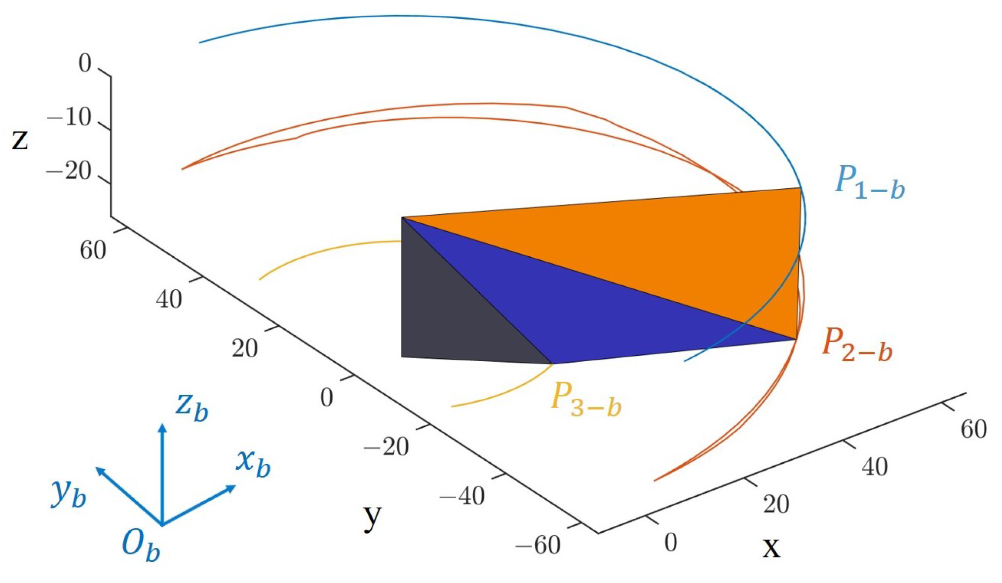
As shown in Figure 1, the shape of the wing in a two-dimensional plane can be represented using parameters in a Cartesian coordinate system: wing height $H_w$, wing length $L_w$, slack angle ${\theta }_s$, and design angle of the carbon fiber spar ${\theta }_{rod1}$ and ${\theta }_{rod2}$. As shown in Figure 1, the points forming the triangular planes in two-dimensional space can be defined as follows:

$$P_{0-2D},P_{1-2D},P_{2-2D},P_{3-2D},P_{4-2D},$$

(1)

and, bringing in the parameters, the position of the point can then be expressed as described below.

$$P_{0-2D}:\left(0,0\right)$$

(2)

$$P_{1-2D}:\left(L_w,0\right)$$

(3)

$$P_{2-2D}:\left(H_w/tan\left({\theta }_{rod1}\right),{-H}_w\right)$$

(4)

$$P_{3-2D}:\left(H_w/tan\left({\theta }_{rod2}\right),{-H}_w\right)$$

(5)

$$P_{4-2D}:\left(-H_w·sin\left({\theta }_s\right),{-H}_w·cos\left({\theta }_s\right)\right)$$

(6)

After the wings are mounted, the position of the points in the wing coordinate system in three-dimensional space can be defined as

$$P_{0-W},P_{1-W},P_{2-W},P_{3-W},P_{4-W}$$

(7)

and the triangular planes Plane1, Plane2, and Plane3 are defined as shown in Figure 2.

At this point, the wing shape does not consider displacement at the wing root, meaning that it assumes the flapping continues in a hovering state without generating average yaw, roll, or pitch moments. At this stage, the shape of each plane remains unchanged and consistent with its shape in the two-dimensional space. The deformed points in three-dimensional space can be represented as follows:

$$P_{0-W}:\left(0,0,0\right)$$

(8)

$$P_{1-W}:\left(L_w,0,0\right)$$

(9)

$$P_{2-W}:\left(x_{2-w},y_{2-w},z_{2-w}\right)$$

(10)

$$P_{3-W}:\left(x_{3-w},y_{3-w},z_{3-w}\right)$$

(11)

$$P_{4-W}:\left(0,0,-H_w\right)$$

(12)

where the positions of $P_{2-W}$ and $P_{3-W}$ can be solved by the system of equations below.

$$\left\{\begin{array}{c}\begin{array}{c}{D}_{02-2D}=D_{02-W}\\ D_{03-2D}=D_{03-W}\end{array}\\ \begin{array}{c}{D}_{12-2D}=D_{12-W}\\ D_{23-2D}=D_{23-W}\end{array}\\ D_{34-2D}=D_{34-W}\end{array}\right.$$

(13)

The distance between point0 and point2 in the two-dimensional Cartesian coordinate system is represented by $D_{02-2D}$, while the distance between point0 and point2 in the three-dimensional wing coordinate system is represented by $D_{02-W}$. The definitions of the other parameters are similar. The reason for establishing this system of equations is that in the multi-plane assumption, due to the presence of veins, the triangular shape of the wing after deformation remains unchanged when divided by veins. Therefore, the distance between the two points in different coordinate systems is equal. Equations (13) can be expanded as follows.

$$\left\{\begin{array}{c}\begin{array}{c}{x}_{2-W}^2+y_{2-W}^2+z_{2-W}^2=L_W^2\\ x_{3-W}^2+y_{3-W}^2+z_{3-W}^2={\left(\frac{H_w}{cos\left({\theta }_{rod1}\right)}\right)}^2\end{array}\\ \begin{array}{c}{\left(x_{2-w}-L_w\right)}^2+{\left(y_{2-w}\right)}^2+{\left(z_{2-w}\right)}^2={\left(L_w-\frac{H_w}{tan\left({\theta }_{rod1}\right)}\right)}^2+{\left(H_w\right)}^2\\ {\left(x_{2-w}-x_{3-w}\right)}^2+{\left(y_{2-w}-x_{3-w}\right)}^2+{\left(z_{2-w}-x_{3-w}\right)}^2={\left(\frac{H_w}{tan\left({\theta }_{rod1}\right)}-\frac{H_w}{tan\left({\theta }_{rod2}\right)}\right)}^2\end{array}\\ {\left(x_{3-w}\right)}^2+{\left(y_{3-w}\right)}^2+{\left(z_{3-w}+H_w\right)}^2={\left(\frac{H_w}{tan\left({\theta }_{rod2}\right)}+H_w·sin\left({\theta }_s\right)\right)}^2+{\left({-H}_w+H_w·cos\left({\theta }_s\right)\right)}^2\end{array}\right.$$

(14)

The number of sub-equations in the system is five, while the number of unknowns to be solved is six. Therefore, it can be concluded that the system of equations is indeterminate, or in other words, that the solution of the equation can be expressed as a function of one of the parameters. This indicates the existence of a certain degree of deformation freedom in the multi-rigid plane fitting, allowing the wing deformation to be represented.

When representing wing deformation using the multi-plane method, the dimensionality of the solution increases with the number of wing veins, making it difficult to represent. In practical design, an increase in the number of wing veins is accompanied by an increase in wing weight, which is unfavorable for the flight characteristics of a flapping aircraft. In this paper, the number of wing veins is set to 2 and the dimensionality of the solution is 1, meaning that the other parameters can be represented by a single parameter.

The most important variables to focus on when solving the unknowns are $y_{2-W}$ and $y_{3-W}$, as they intuitively represent the attack angle of plane1 and plane2 when flapping. For ease of analysis, $y_{2-W}$ is set as the independent variable parameter; a graphical analysis is conducted to examine its relationship with under different slack angles, as shown in Figure 3.

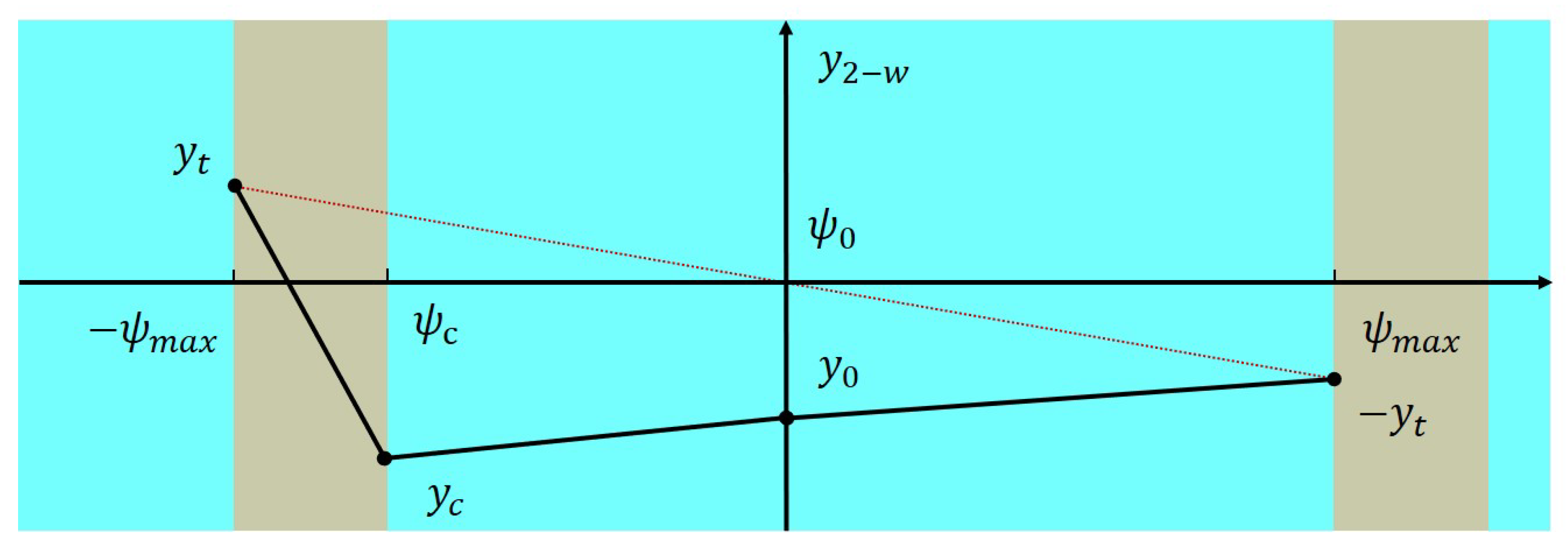
From the figure, it can be observed that the feasible range of $y_{3-W}$ increases with the increase in the slack angle. Meanwhile, $y_{3-W}$ shows a trend of first increasing and then decreasing with the increase of $y_{2-W}$. Prior to reaching the maximum value, the angle between plane1 and plane2 is negative, indicating that only when the value of $y_{2-W}$ starts to decrease does the entire wing begin to exhibit a naturally curved and full shape. Combining with the definition of the wing in an inflated state, the feasible range of $y_{2-W}$ under different slack angles is derived as shown in Figure 4.

As shown in Figure 5, under different values of $y_{2-W}$, the shape of the wing in the three-dimensional space varies. After selecting appropriate values of $y_{2-W}$, the shape representation of the wing using the multi-plane method closely approximates the wing’s installed shape in its natural state, as shown in Figure 6. The main difference lies in the smooth curve of the wing’s lower edge in its natural state, while the lower edge represented by the multi-plane method consists of line segments, resulting in some numerical discrepancies between the two.

In existing hovering flapping-wing prototypes, a two-degrees-of-freedom flapping mechanism is commonly used to control the flapping and rotation of the wings. During hovering flight, the wings only undergo reciprocating flapping. The flapping process can be divided into a translational stage and a passive wing flipping stage, with the translational aerodynamic force accounting for approximately 70% of the total lift. During the translational stage, the wings are under tension due to the aerodynamic forces. As shown in Figure 5, different wing deformations can be achieved by adjusting the value of $y_{2-W}$ after determining the slack angle, while the wing’s shape at various positions during actual flapping can be obtained by combining the actual flapping angle position. By analyzing the morphological changes of the wing during flapping, aerodynamic forces and drag can be analyzed and various parameters in wing design can be adjusted based on optimization objectives in order to guide the design of the wing.

3. Kinematic Analysis of Wings Based on the Multi-Plane Simulation Method

By adjusting the parameters $y_{2-W}$, the shape of the wing can be flexibly adjusted. Observing the phenomenon during actual flapping, it is found that the shape of the wing varies at different positions due to factors such as flapping angular velocity and inertia. In addition, there is flexible deformation during wing flipping. As the translational velocity of the wing during flipping is relatively low and the flexible deformation has a significant impact, appropriate adjustments need to be made to the multi-plane method based on the invariant plane area. This section introduces the kinematic analysis of the wing based on the multi-plane simulation method along with the modified data of $y_{2-W}$ based on the position and flapping angular velocity in order to simulate the deformation of the wing during flapping and prepare for calculating the aerodynamic forces of the wing.

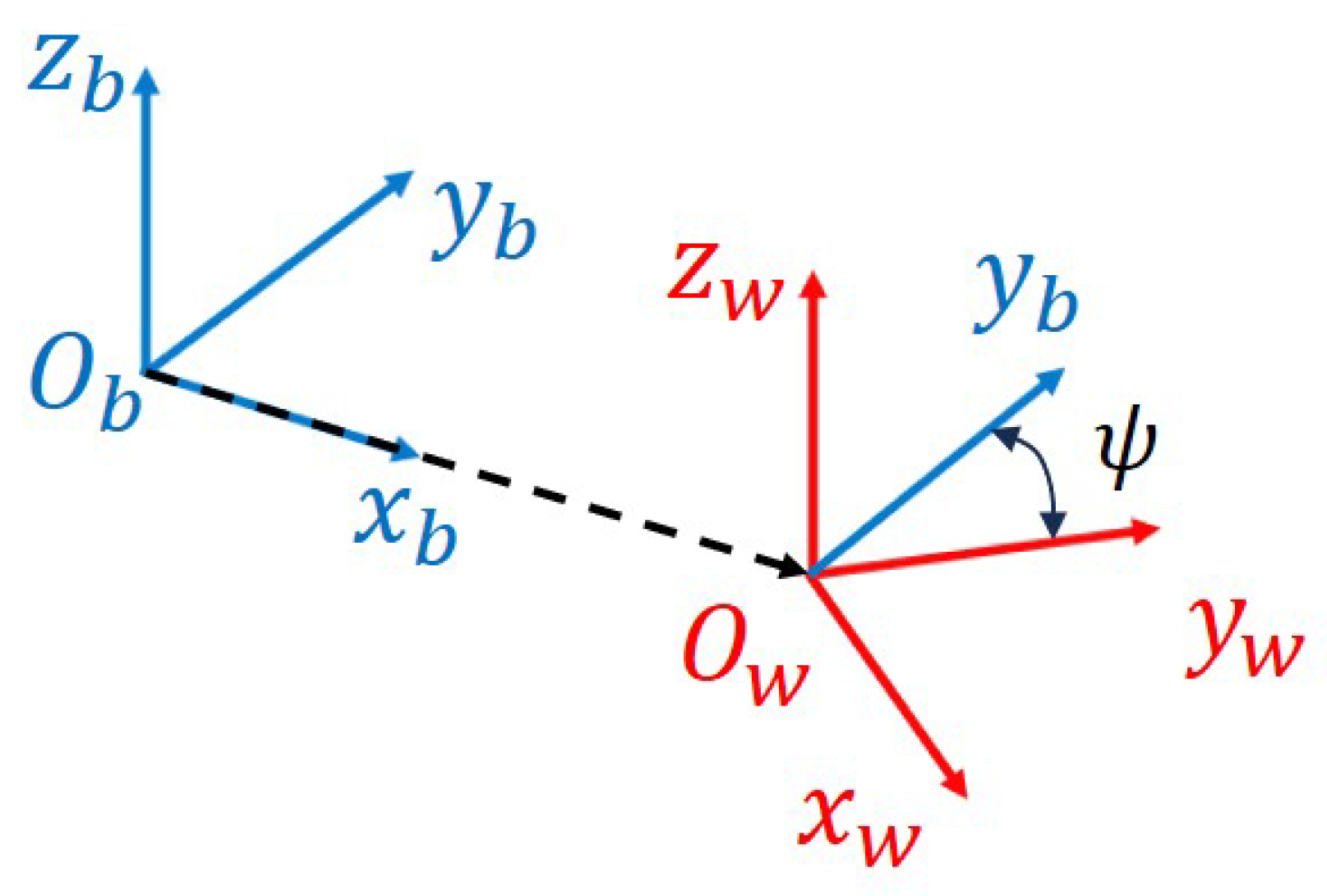
Before simulating the deformation of the wing during flapping, it is necessary to describe the shape of the wing in the body coordinate system. In the previous section, we defined the shape of the wing in the right wing coordinate system; as shown in Figure 7, both the right wing coordinate system and the body coordinate system are right-handed coordinate systems, with their z-axis directions the same and pointing upwards. The positive direction of the y-axis of the body coordinate system is defined as the forward direction of the body, and the positive direction of the x-axis is defined as the direction of the right wing at the flapping center position, with the coordinate origin located at the center of gravity of the body. The origin of the right wing coordinate system is located at the mounting root point of the right wing, with its x-axis direction the same as the direction of the wing spar. In summary, the position $P_W$ of any point in the right wing coordinate system can be expressed as $P_b$ in the body coordinate system, as follows:

$$P_b=R_{w\to b}{P}_w-O_b{O}_w.$$

(15)

The vector from the origin of the body coordinate system to the origin of the wing coordinate system, represented in the body coordinate system, is denoted as $O_b{O}_W$. The rotation matrix from the wing coordinate system to the body coordinate system can be expressed as $R_{w\to b}$, where $\psi$ represents the rotation angle around the z-axis. Because the z-axis directions of the two coordinate systems are the same, the rotation matrix can be represented by Equation (16):

$$R_{w\to b}=\left[\begin{array}{ccc}cos\psi & -sin\psi & 0\\ sin\psi & cos\psi & 0\\ 0& 0& 1\end{array}\right].$$

(16)

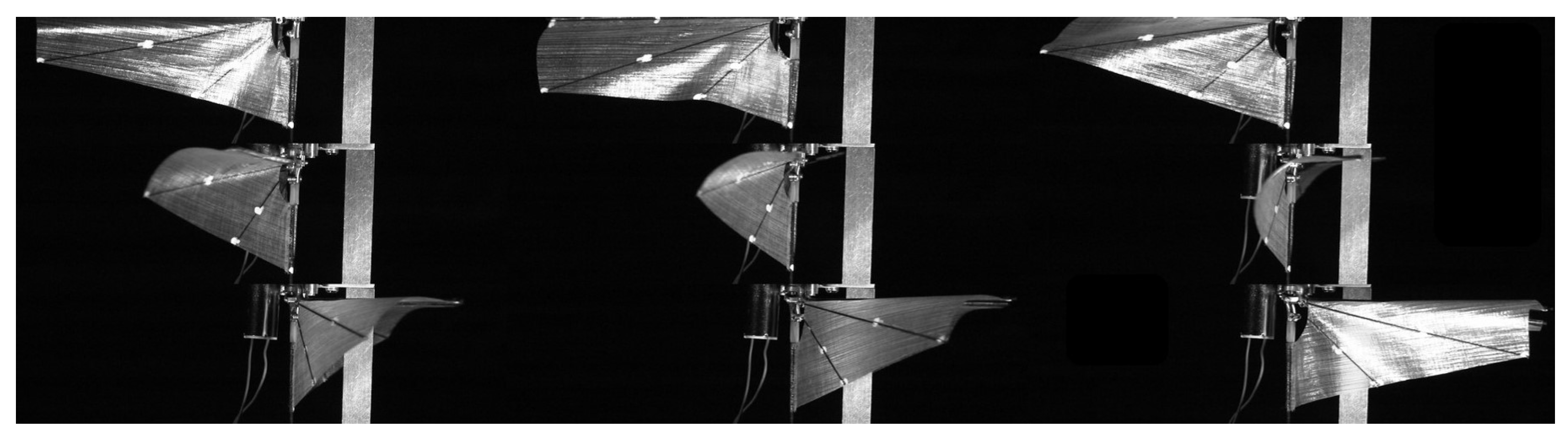
As mentioned above, by combining previous research [52] and actual wing motion images captured under high-speed photograph in Figure 8, it can be inferred that the shape of the wing varies at different positions. Therefore, before analyzing the kinematics of the wing using the multi-plane simulation method, it is necessary to define the shape of the wing at each position. Referring to previous research [47,48], we consider a linear fitting method in the simulation definition, which defines a linear representation of the wing by defining key points between the leading edge and the trailing edge of the flapping motion.

As shown in Figure 9, taking half of a flapping cycle as an example, the flapping angle of the wing ranges from $-{\psi }_{max}$ to ${\psi }_{max}$. Within the range of angles from ${\psi }_c$ to ${\psi }_{max}$, the multi-plane method can be used for equivalence, as wing completes a full rotation from ${\psi }_c$, allowing for multi-plane equivalence. However, within the range of angles from $-{\psi }_{max}$ to ${\psi }_c$ the wing is in the rotation phase and its shape undergoes significant changes, making it inappropriate to consider it as a flat plane with an unchanged shape. Considering the symmetry of the wing before and after flapping, the values of $y_{2-W}$ at the two moments are opposite to each other; furthermore, based on the analysis of actual shooting of the wing flapping, it is observed that when the wing has just completed the reversal. Thus, the angle of attack of plane1 is the smallest when the flapping angle at ${\psi }_c$, indicating the maximum value of $\left|y_{2-w}\right|$. While it gradually decreases afterwards, the overall change is not significant.

The wing undergoes significant deformation during the wing reversal, making it impossible to simulate the wing deformation by considering a plane with an unchanged shape. Instead, a direct definition is chosen by fitting its flapping shape using $y_{2-W}$, $z_{2-W}$, $y_{3-W}$, $z_{3-W}$, and so on. The method is to combine the last positions of $P_{2-W}$ and $P_{3-W}$ in the first half of the flapping cycle by considering their Y values in combination with symmetry, then linearly fitting the intermediate process to obtain the defining multi-plane parameters used to fit the wing reversal. By combining the simulation methods mentioned above, the various parameters can be expressed using formulas. When the flapping angle $\psi$ satisfies ${\psi }_c\le \psi \le {\psi }_{max}$, we have

$$y_{2-w}=\frac{{-y}_t-y_c}{{\psi }_{max}-{\psi }_c}\psi -y_t,{\psi }_c\le \psi \le {\psi }_{max}.$$

(17)

In this case, the values of $z_{2-w}$, $y_{3-w}$, $z_{3-w}$ can be obtained using the value of $y_{2-w}$, which can be solved by the multi-plane simulation method with the system of equations in (14).

When the flapping angle $\psi$ satisfies $-{\psi }_{max}\le \psi \le {\psi }_c$, we have

$$\left\{\begin{array}{c}\begin{array}{c}{y}_{2-w}=\frac{y_t-y_c}{-{\psi }_{max}-{\psi }_c}\psi +y_c-\frac{y_t-y_c}{-{\psi }_{max}-{\psi }_c}{\psi }_c\\ z_{2-w}=\frac{z_t-z_c}{-{\psi }_{max}-{\psi }_c}\psi +z_c-\frac{z_t-z_c}{-{\psi }_{max}-{\psi }_c}{\psi }_c\end{array}\\ \begin{array}{c}{y}_{3-w}=\frac{y_{t-3}-y_{c-3}}{-{\psi }_{max}-{\psi }_c}\psi +y_{c-3}-\frac{y_{t-3}-y_{c-3}}{-{\psi }_{max}-{\psi }_c}{\psi }_c\\ z_{3-w}=\frac{z_{t-3}-z_{c-3}}{-{\psi }_{max}-{\psi }_c}\psi +z_{c-3}-\frac{z_{t-3}-z_{c-3}}{-{\psi }_{max}-{\psi }_c}{\psi }_c\end{array}\end{array}\right.$$

(18)

where $\left|y_c\right|$ and $\left|y_t\right|$ are the maximum value $y_{max}$ and minimum value $y_{min}$ that allow the formation of a full plane, as shown in Figure 4. Multiplying by a 0.95 margin, this can be represented as

$$\left\{\begin{array}{c}\left|y_c\right|=y_{max}-0.05\left(y_{max}-y_{min}\right),\\ \left|y_t\right|=y_{min}+0.05\left(y_{max}-y_{min}\right).\end{array}\right.$$

(19)

Points $\left(x_t,y_t,z_t\right)$ and $\left(x_{t-3},y_{t-3},z_{t-3}\right)$ are the last positions of $P_{2-W}$ and $P_{3-W}$ in the right wing coordinate system at the end of the first half of the flapping cycle, while $\left(x_c,y_c,z_c\right)$ and $\left(x_{c-3},y_{c-3},z_{c-3}\right)$ are the positions of points $P_{2-W}$ and $P_{3-W}$ after the wing is flipped over. Points $\left(x_t,y_t,z_t\right)$ and $\left(x_{t-3},y_{t-3},z_{t-3}\right)$ can be obtained by solving $y_{2-w}=-y_t$ and inverting the value of y.

Figure 10 shows the schematic diagram of the wing shape in the body coordinate system after simulation using the multi-plane method. The three curves in Figure 10 represent the motion trajectories $P_{1-b}$, $P_{2-b}$, $P_{3-b}$ in the body coordinate system, where $\psi ={-\psi }_{max}cos\left(2\pi ft\right)$ represents trajectory of the leading edge spar, which is driven by a string-based mechanism and has been found in previous studies to have a trajectory similar to a standard sine wave [4] (shown in Figure 11). For simplicity, it is directly represented here as a sine wave. Figure 12 shows the schematic diagram of the wing shape at different positions in the body coordinate system, as obtained by linear fitting using different values of $y_{2-W}$ at various locations compared with high-speed photography. By comparing the diagram with the wing captured in real footage, it can be observed that it exhibits a similar trend to the actual wing movement in terms of motion. By combining partial recorded flapping motion parameters and modifying the values of $y_{2-W}$ at different time points, including the start and end points of the flip, a more accurate fitting of the actual flapping trajectory can be achieved.

By comparing the shape variations of the simulated wing with the actual flapping motion, it can be observed that the multi-plane simulation method provides a good fit to the actual wing flapping process. Compared to the analysis using the blade element theory, the multi-plane simulation method is more morphologically accurate in representing the flapping trajectory. It takes into account the three-dimensional deformation of the wing, while the blade element theory assumes the wing to be planar, resulting in the loss of morphological parameters. By combining the multi-plane simulation method with the blade element theory, more comprehensive aerodynamic information of the wing can be obtained, providing a more accurate basis for wing design. Moreover, this approach is simpler compared to the fluid–structure coupling calculations for capturing the flexible deformation of the wing. By combining the multi-plane simulation method with the blade element theory, it is possible to perform simulation analysis on the aerodynamic forces during wing flapping.

4. Aerodynamic Analysis Based on the Multi-Plane Simulation Method

The kinematic simulation of the wing using the multi-plane method enables the modification of wing by adjusting parameters, which is closer to the realistic flapping process than the blade element theory assuming a single rigid plane. After obtaining the wing’s deformation during the flapping trajectory, aerodynamic analysis of the wing can be performed by combining it with the quasi-steady blade element theory.

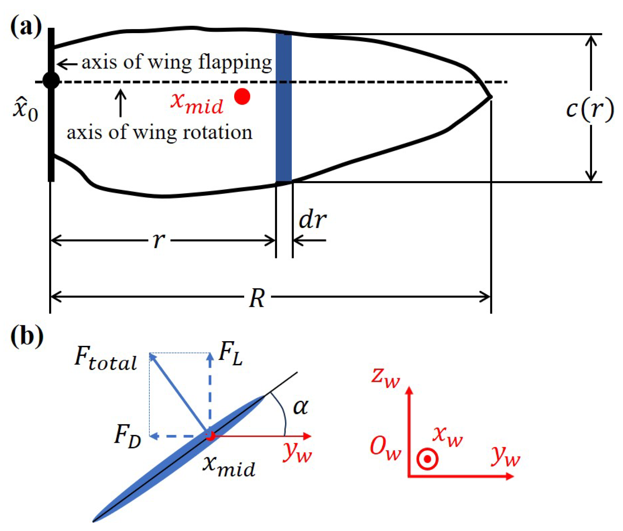
In aerodynamic analysis, the conventional blade element theory typically divides a single rigid-plane wing into multiple blade elements and calculates the aerodynamic forces for each blade element, which are then summed. Figure 13a illustrates the schematic diagram of the classical blade element theory for calculating aerodynamic forces on a single rigid plane wing. In the diagram, $dr$ represents the blade width, r denotes the distance of the current blade element from the flapping axis, R represents the spanwise length of the wing, $c\left(r\right)$ represents the chord length of the blade element, ${\widehat{x}}_0$ represents the intersection point between the rotation axis and the flapping axis, and $x_{mid}$ represents the geometric center of the wing. Neglecting the wing’s vertical flapping motion, the flapping plane of the wing coincides with the $XY$ plane of the wing coordinate system and the body coordinate system with an angle $\alpha$, which can be called the angle of attack between the wing surface and the flapping plane, as shown in Figure 13b.

Based on investigation of the quasi-steady aerodynamic model for hovering flapping-wing aircraft, the aerodynamic forces can be categorized into translational aerodynamic forces, rotational aerodynamic forces, aerodynamic forces induced by added mass, inertial forces, and forces resulting from special aerodynamic effects [1,2,3]. Among these, the aerodynamic forces caused by clap and fling contribute the most to the forces resulting from special effects. While these have a significant impact on hovering flight with flapping amplitudes greater than 180° [5,6], they have a negligible effect on flapping-wing aircraft where the wings do not make contact during the flipping motion, and can be disregarded. Similarly, the effects of delayed stall [7,8,9,10] and wake capture [11,12,13] are not often considered in quasi-steady aerodynamic models. The inertial forces are related to the wing mass and flapping angular velocity; however, due to the front–back symmetry of flapping, they mutually cancel out within one cycle and can be omitted from the analysis. Therefore, the translational aerodynamic force and the rotational aerodynamic force are the forces that have the greatest impact on the hovering flapping wing. By combining the defined parameters and previous research, the translational aerodynamic force $F_{tr}^{\prime }$ of a single blade element can be expressed as

$$F_{tr}^{\prime }=F_{Ltr}^{\prime }+F_{Dtr}^{\prime },$$

(20)

where $F_{Ltr}^{\prime }$ represents the translational lift force and $F_{Dtr}^{\prime }$ represents the translational drag force, provided by

$$F_{Ltr}^{\prime }=\frac{1}{2}\rho C_L\left(\alpha \right)c\left(r\right){\left(\dot{\psi }r\right)}^{2}dr,$$

(21)

$$F_{Dtr}^{\prime }=\frac{1}{2}\rho C_D\left(\alpha \right)c\left(r\right){\left(\dot{\psi }r\right)}^{2}dr,$$

(22)

where $\rho$ represents the air density, $\dot{\psi }$ is defined as the flapping wing’s angular velocity, $\dot{\psi }r$ is the translational velocity of the blade section at a distance r from the flapping axis, and $C_L\left(\alpha \right)$ and $C_D\left(\alpha \right)$ are the lift and drag coefficients, respectively, obtained from experimental data. Based on previous research [36,37,38], for flapping-wing aircraft at the decimeter scale, the following equations can be used for approximate fitting:

$$C_L\left(\alpha \right)=0.255+1.58sin(2.13\alpha -7.2),$$

(23)

$$C_D\left(\alpha \right)=1.92-1.55sin(2.04\alpha -9.28).$$

(24)

In some studies, a small difference between the geometric angle of attack and the actual angle of attack has been considered, referred to as the induced angle $\beta$, which has a small value. In this paper, consistent with most of the literature, $\beta$ is assumed to be 0, implying that the geometric angle of attack is equal to the actual angle of attack.

The rotational aerodynamic force of a single blade can be expressed as

$$F_{rot}^{\prime }=\rho C_{rot}\dot{\alpha }(\dot{\psi }r)c^2\left(r\right)dr,$$

(25)

with the value of the rotational aerodynamic coefficient $C_{rot}$ being dependent on the position of the axis of rotation, which can be expressed as follows:

$$C_{rot}=\pi \left(0.75-x_0\right)$$

(26)

where the parameter $x_0$ represents the dimensionless distance of the axis of rotation, which is dependent on the wing morphology and the position of the axis of rotation. In nature, birds and insects typically have values of $x_0$ ranging from 0.25 to 0.35; however, in the majority of existing flapping-wing prototypes, where the leading edge serves as the axis of rotation, the dimensionless position of the axis of rotation $x_0$ can be set to 0. Thus, the aerodynamic forces resulting from the rotation of a single blade can be expressed as follows:

$$F_{rot}^{\prime }=\frac{3}{4}\pi \rho \dot{\alpha }(\dot{\psi }r)c^2\left(r\right)dr.$$

(27)

Similar to the direction of the force indicated in Figure 13b, the direction of the rotational aerodynamic force is perpendicular to the wing surface, and can be decomposed into the rotational lift $F_{Lrot}^{\prime }$ and rotational drag $F_{Drot}^{\prime }$, which can be expressed as follows:

$$F_{Lrot}^{\prime }=F_{rot}^{\prime }cos\left(\alpha \right)=\frac{3}{4}\pi \rho \dot{\alpha }(\dot{\psi }r)c^2\left(r\right)cos\left(\alpha \right)dr,$$

(28)

$$F_{Drot}^{\prime }=F_{rot}^{\prime }sin\left(\alpha \right)=\frac{3}{4}\pi \rho \dot{\alpha }(\dot{\psi }r)c^2\left(r\right)sin\left(\alpha \right)dr.$$

(29)

The source of the added mass aerodynamic force is the reaction force exerted by the surrounding air on the wing during the flapping motion. The added mass aerodynamic force of a single blade can be expressed as follows:

$$F_{add}^{\prime }=-\rho S_{air}{a}_{air}dr$$

(30)

where $S_{air}dr$ represents the equivalent volume of air on the blade and $S_{air}$ represents the equivalent surface area of the modified cylinder. These can be expressed as

$$S_{air}=\frac{\pi }{4}{c}^2\left(r\right),$$

(31)

where $a_{air}$ is the acceleration of the considered part of the air, which can in turn be expressed as

$$a_{air}=\left(r\ddot{\psi }+\frac{c\left(r\right)}{2}{\psi }^{2}cos\left(\alpha \right)\right)sin\left(\alpha \right)+\frac{c\left(r\right)}{2}\ddot{\alpha }.$$

(32)

The aerodynamic forces caused by added mass are similar to the aerodynamic forces resulting from rotation, as they both act perpendicularly to the wing surface. Similarly, they can be decomposed into the lift $F_{Ladd}^{\prime }$ and drag $F_{Dadd}^{\prime }$, which can be expressed as follows:

$$F_{Ladd}^{\prime }=-\frac{\pi \rho }{4}{c}^2\left(r\right)\left[\left(r\ddot{\psi }+\frac{c\left(r\right)}{2}{\psi }^{2}cos\left(\alpha \right)\right)sin\left(\alpha \right)+\frac{c\left(r\right)}{2}\ddot{\alpha }\right]cos\left(\alpha \right)dr,$$

(33)

$$F_{Dadd}^{\prime }=-\frac{\pi \rho }{4}{c}^2\left(r\right)\left[\left(r\ddot{\psi }+\frac{c\left(r\right)}{2}{\psi }^{2}cos\left(\alpha \right)\right)sin\left(\alpha \right)+\frac{c\left(r\right)}{2}\ddot{\alpha }\right]sin\left(\alpha \right)dr.$$

(34)

By integrating the translational aerodynamic force, rotational aerodynamic force, and added mass-induced aerodynamic force on a single blade, the quasi-steady model under the assumption of a rigid flat plane can be obtained. This model represents the transient aerodynamic forces during wing flapping. The transient lift $F_L$ and transient drag $F_D$ can be expressed as follows:

$$F_L=\underset{0}{\overset{R}{\int }}\left(F_{Ltr}^{\prime }+F_{Lrot}^{\prime }+F_{Ladd}^{\prime }\right),$$

(35)

$$F_D=\underset{0}{\overset{R}{\int }}\left(F_{Dtr}^{\prime }+F_{Drot}^{\prime }+F_{Dadd}^{\prime }\right).$$

(36)

From the parameters in the above equations, it can be observed that under the assumption of a rigid flat plane in the quasi-steady model, the aerodynamic forces of wing flapping can be estimated when the morphological parameters of the wing such as the chord length $c\left(r\right)$, angle of attack $\alpha$, and flapping angular velocity $\dot{\psi }$ are known. Under the assumption of a rigid flat plane, the angular velocities, angles of attack, and their derivatives for each blade on the wing are assumed to be the same; however, during the actual flapping process of a wing, the wing’s flexibility and nonlinear characteristics may cause variations in wing’s deformation and aerodynamic force distribution. Therefore, the multi-plane method can be employed to more accurately simulate the wing’s motion and deformation. By dividing the wing into multiple planes and assuming that the angular velocities of these rigid planes are the same as the leading-edge angular velocity of the wing while considering the differences in the angles of attack and their derivatives for each plane, the aerodynamic forces of different sections of the wing can be calculated more precisely.

Figure 14 presents a quasi-steady aerodynamic simulation method incorporating the multi-plane approach. The figure depicts a schematic view of the wing observed from the opposite direction of the Y-axis in the wing coordinate system after determining the wing’s shape in three-dimensional space. Similar to the analysis of a single rigid plane, the wing is divided into multiple blade segments along the span direction, each with a width of $dr$; however, in contrast, these blade segments reside on planes in three-dimensional space. This implies that the angle of attack $\alpha$ varies for each blade segment on different planes, necessitating a separate analysis for each plane. When calculating the aerodynamic forces for each blade segment, it is essential to consider the current wing shape, as the morphological parameter $c\left(r\right)$ varies with time at different positions along the wing. Therefore, the analysis needs to be conducted in conjunction with the wing’s present morphology. Additionally, as depicted in Figure 14, the number of intersections between the sampled blade segments (which serve as the reference in the wing coordinate system’s $YZ$ plane) and the planes differs due to the varying values of r.

The quasi-steady aerodynamic analysis using the multi-plane approach can be approximated as the superposition of quasi-steady aerodynamic analyses conducted on multiple planes. However, an issue arises when analyzing the additional aerodynamic forces caused by the overlapping of partial air volumes between different blade segments, as illustrated in Figure 15. It is challenging to determine whether it is necessary to treat this overlap as an equivalent longer blade segment for the calculation of additional mass-induced aerodynamic forces. Nevertheless, previous studies [40,42,43] have shown that the aerodynamic forces caused by additional mass are relatively small compared to the translational and rotational terms, suggesting that they can be approximated so as to have no significant impact on the results. Additionally, it is worth noting that we have omitted the potential interplay between the translational aerodynamic forces and rotational aerodynamic forces across different planes. Whether this simplification is permissible in actual physical analysis requires further verification in subsequent research. In summary, under the assumption of three planes, the quasi-steady unsteady aerodynamic forces using the multi-plane approach can be expressed as follows:

$$F_{Lall}=F_{Lp1}+F_{Lp2}+F_{Lp3}\approx F_{Ltrp1}+F_{Ltrp2}+F_{Ltrp3}+F_{Lrotp1}+F_{Lrotp2}+F_{Lrotp3},$$

(37)

$$F_{Dall}=F_{Dp1}+F_{Dp2}+F_{Dp3}\approx F_{Dtrp1}+F_{Dtrp2}+F_{Dtrp3}+F_{Drotp1}+F_{Drotp2}+F_{Drotp3}.$$

(38)

The instantaneous lift and drag obtained through the multi-plane approach are denoted as $F_{Lall}$ and $F_{Dall}$, respectively, while $F_{Lp1}$ and $F_{Dp1}$ respectively represent the instantaneous lift and drag of plane1 obtained using the quasi-steady aerodynamic model. The definitions for the remaining variables are similar.

When calculating aerodynamic forces using the quasi-steady aerodynamic model, the derivative of the angle of attack is essential; however, when computing the angle of attack and its derivative, discontinuities in the derivative may occur at inflection points due to the linear fitting method used to define points on the plane, as shown in Figure 9. This can lead to singular values in the aerodynamic force calculations. To address this issue, it is necessary to apply a smoothing technique to the fitted value function in order to ensure that the derivative of the angle of attack does not exhibit extreme values.

The optimized values of $y_{2-w}$ compared with linear fitting and changed based on the flapping angle are shown in Figure 16, which illustrates the cyclic behavior within one flapping period. Inspired by the sinusoidal modulation of the flapping trajectory in wingbeat modulation techniques [53], we employed trigonometric functions in the simulation process instead of the original piecewise linear fitting method to ensure the continuity of the derivative and second derivative at the inflection points. Through trigonometric function modulation, the original fitting Equation (17) and fitting Equation (18) are transformed into the following.

$$\left\{\begin{array}{c}{y}_{2-w}=\frac{y_t+y_c}{2}-\frac{y_t-y_c}{2}sin\left(\pi \frac{\psi -\frac{{\psi }_c-{\psi }_{max}}{2}}{{\psi }_c+{\psi }_{max}}\right),-{\psi }_{max}\le \psi \le {\psi }_c\\ y_{2-w}=\frac{-y_t+y_c}{2}+\frac{{-y}_t-y_c}{2}sin\left(\pi \frac{\psi -\frac{{\psi }_c+{\psi }_{max}}{2}}{{\psi }_{max}-{\psi }_c}\right),{\psi }_c\le \psi \le {\psi }_{max}\end{array}\right.$$

(39)

After applying trigonometric function smoothing to the $y_{2-w}$ trajectory, extreme values in the derivative and second derivative no longer occur. By utilizing the flapping trajectory simulation method described earlier in conjunction with quasi-steady aerodynamic analysis using the multi-plane approach, it is possible to simulate the transient aerodynamic forces within one flapping period. As shown in Figure 17, transient aerodynamic analysis was conducted for a single wing using the simulation parameters provided in

Table 1. Values of parameters.

Parameters	Data
Length of wing $L_w$	65 mm
Height of wing $H_w$	26 mm
Installation angle of rod1 ${\theta }_{rod1}$	23°
Installation angle of rod1 ${\theta }_{rod2}$	50°
Flapping amplitude	160°
Flapping frequency	35 Hz
$y_t$	15 mm
$y_c$	−22 mm
${\psi }_{max}$	80°
${\psi }_c$	−50°
Flapping frequency	35 Hz
Reynolds number	2.2321 × 104
Strouhal number	0.0716

.

As shown in Figure 17, the transient aerodynamic simulation results for one wing within a single period were analyzed using the multi-plane approach and quasi-steady aerodynamic model. The results include the lift and drag components of the aerodynamic forces in Figure 17a,c as well as the contributions of each plane to the lift and drag in Figure 17b,d. Based on the data in the figures, the following conclusions can be drawn. Regarding the aerodynamic lift, the translation component provides the main contribution while the contribution of the rotation component is relatively small, as shown in Figure 17a. At the wing reversal point, which is the half-period position, the rotation component contributes partially to the lift. Different planes exhibit varying contributions to the lift, with plane1 having the largest contribution and plane2 and plane3 having smaller contributions, as shown in Figure 17b. Therefore, the translational force of plane1 plays a crucial role in lift generation. In terms of aerodynamic drag, the translation component again dominates. As shown in Figure 17c, during wing reversal, the rotation component provides drag in the opposite direction to the motion due to the wing’s deformation, thereby reducing the overall drag. It can be seen in Figure 17d that in terms of the drag distribution plane1 and plane2 account for the majority, while the contribution of plane3 is minimal. This aligns with our initial expectation that plane3 would be closer to the axis of rotation and have a lower translational velocity, resulting in negligible aerodynamic effects. This phenomenon is evident when observing the wing shapes of most insects in nature, where the wings typically narrow towards the wing root. This design reduces inertial forces while minimizing the impact of aerodynamic effects due to a missing area of wing.

Figure 18 presents a comparison between the simulated and experimentally measured lift at different frequencies of mean lift, expressed in units of gf and lift coefficient. The lift coefficient can be computed as follows:

$$C_L=\frac{2F_L}{\rho {\stackrel{-}{u}}^{2}S}$$

(40)

where $F_L$ is the average lift expressed in Newtons, $\rho$ represents air density, $\stackrel{-}{u}$ represents average the flapping speed of the wing tips, and S represents the equivalent area of the wings.

The wing parameters used in the simulation are consistent with those in Table 1, with the unmarked parameter being the wing’s slack angle, which has a value of 13.5°. By comparing the results in Figure 18, it can be observed that there is minimal difference between the simulated data and the experimental results within the selected frequency range. Meanwhile, through comparison with the single-plane blade element method, it can be seen that the multi-plane method is relatively accurate in simulating lift. Additionally, more precise simulations can be achieved by adjusting the wing’s deformation parameters at different time points. Therefore, the quasi-steady aerodynamic model analyzed using the multi-plane approach exhibits high accuracy.

With increasing flapping frequency, a growing divergence is observed between the experimental data and both the multi-plane and single rigid plane simulation data regarding the average lift. This discrepancy likely arises from the omission of clap and fling in the simulation models, as delineated earlier. Previous studies have indicated that the interaction at the wingtips can initiate this mechanism, potentially contributing up to 30% of the total lift. As the actual flapping frequency escalates, the inertia of the wings augments the flapping amplitude, thereby enhancing the lift generated by clap and fling. However, quasi-steady-state models neglect this lift source, leading to an expanding deviation between simulation results and experimental observations. This amplifies the limitations of quasi-steady-state models in capturing complex aerodynamic behaviors. Incorporating these unique aerodynamic effects inherent in the flapping process can significantly narrow the gap between simulated and empirical values. In this context, our study estimates that for flapping frequencies up to 40 Hz, the quasi-steady-state aerodynamic model utilizing the multi-plane approach aligns with the actual measured data in predicting average lift with a 90% degree of similarity. However, with further frequency elevation, incorporating additional aerodynamic forces previously disregarded in simulations may be imperative in order to more precisely mirror the actual findings.

The lift-to-power ratio is a parameter of great interest in the design of flapping-wing micro air vehicles. Typically measured in g/W, it evaluates the generated lift efficiency per unit power of the wing. Based on previous research [24,47,48] and the aforementioned analysis, it is known that the main sources of lift and drag in flapping flight are the translational components, which are closely related to the power consumed by the wing in generating lift and overcoming aerodynamic drag during translation. By employing the multi-plane approach and quasi-steady aerodynamic model, the variation in the lift-to-power ratio can be further analyzed under different slack angles and wing deformation conditions, providing a valuable reference for wing design.

Figure 19 illustrates the aerodynamic effects of wing translation, where the variations in transient lift, transient drag, transient power, and lift-to-power ratio with respect to $y_{2-w}$ under different slack angles are displayed separately in Figure 19a–d. The transient power in the translational effect can be approximated as the power consumption of the wing, as the wing only moves in the drag direction. Its calculation can be expressed as follows:

$$P_{Dtr}=\underset{0}{\overset{R}{\int }}{F}_{Dtr}^{\prime }\dot{\psi }r=\underset{0}{\overset{R}{\int }}\frac{1}{2}\rho C_D\left(\alpha \right)c\left(r\right){(\dot{\psi }r)}^{3}dr$$

(41)

and the lift-to-power ratio $\eta$ can be simplified as

$$\eta =\frac{F_{Ltr}}{P_{Dtr}}.$$

(42)

As mentioned earlier, under different slack angles, the range of $y_{2-w}$ values in the wing coordinate system varies to ensure a full wing shape. With an increasing slack angle, the translational aerodynamic lift of the wing shows the increasing trend displayed in Figure 19a, while the drag and drag power exhibit a decreasing trend, as shown in Figure 19b,c. Consequently, the lift-to-power ratio increases, indicating an improvement in wing efficiency. However, at the same slack angle, as shown in Figure 19a, the trend of lift variation is related to the absolute value of $y_{2-w}$. This is because under different slack angles the wing’s angle of attack changes differently around 45°, where the lift coefficient reaches its maximum value. In contrast, in Figure 19b,c it can be seen that the drag increases as the absolute value of $y_{2-w}$ decreases, because the drag coefficient increases with increasing angle of attack. The variation in wing shape is closely related to the slack angle. By combining this variation, a simulated schematic diagram of the $y_{2-w}$ values and lift-to-power ratios under different slack angles can be plotted, as shown in Figure 19d. After reaching a certain range of slack angles, the wing exhibits a full shape, characterized by the maximum lift-to-power ratio. Additionally, it is worth mentioning that the analysis of the lift-to-power ratio for the same wing at different frequencies reveals a decrease in wing efficiency with increasing frequency, as shown in Figure 20. This is because the translational lift is proportional to the square of the frequency, while the translational drag power is proportional to the cube of the frequency.

By combining the multi-plane simulation method with the classical blade element theory, the aerodynamic forces of the wing at different positions, velocities, and shapes can be calculated while taking into account the different deformations of the wing at different locations. Compared to the single-plane blade element method, the multi-plane method can more accurately reflect the wing’s deformation during flapping and can calculate the aerodynamic forces more accurately. Additionally, by incorporating the parameters used in wing design, the multi-plane method can analyze the aerodynamic effects of the twist angle on the wing during two-dimensional plane design. By combining multi-plane aerodynamic analysis with optimization methods, the relationship between the slack angle and lift-to-power ratio can be studied, optimal design parameters can be identified, and the efficiency of the wing under different deformations can be explored, providing guidance for the design and optimization of wing shapes.

5. Experiments and Analysis

To observe the shape variations of wings during flapping, we captured the actual flapping wings using high-speed photography. The schematic diagram of the testing environment is shown in Figure 21. Synchronized high-speed video captures of the actual wings were taken from different angles. The black dots labeled as point1–point7 in Figure 22 represent marker positions. The purpose of these markers was to calculate the spatial positions using three-dimensional video processing software after the shoot. The markers were placed on three carbon fiber rods (rod1–rod3) and the root point of the wing, dividing the wing into three sections. These markers were intended to facilitate our analysis of the motion of the carbon fiber rods during data processing in order to determine the fitted plane shape of the motion. The parameters of the captured footage are listed in

Table 2. Values of experimental parameters.

Parameters	Data
Length of wing $L_w$	65 mm
Height of wing $H_w$	26 mm
Slack angle ${\theta }_s$	13.5°
Installation angle of rod1 ${\theta }_{rod1}$	20°
Installation angle of rod1 ${\theta }_{rod2}$	50°
Shooting frame rate	5000 Hz
Voltage of motor	4.6 v
Flapping frequency	28.7 Hz

.

The structure used to drive the wings is based on the previously designed string-based mechanism [4], which has the advantage of producing wing flapping angles similar to a standard sine wave and lower flapping angular velocities at the ends of the flapping stroke. The processed results of the data captured at 28.7 Hz are shown in Figure 23. Figure 23a reflects the variations in the flapping angles of the three carbon fiber rods observed from the positive z-axis direction, while Figure 23b shows the differences between them. The changes in the angle of attack of the fitted flapping plane using points 0,2,4, 0,4,6, and 0,6,7 are presented in Figure 24. Due to the discontinuity in the interpolated points, spikes may be present in the waveform; therefore, Gaussian averaging was applied to the data to smooth out any spikes. The displayed images are the processed ones.

From Figure 23, it can be observed that Rod1, which is the leading edge rod, consistently exhibits a phase lead with respect to rod2 and rod3. The phases of rod2 and rod3 are close to each other, indicating that, when observed from the positive z-axis direction, plane2 and plane3 can be considered to lie in the same plane most of the time. Additionally, plane3 exhibits greater bending during wing flipping, indicating more pronounced undulations compared to plane2.

Through analysis of the time-varying angle of attack for the three planes in Figure 24, it can be observed that plane1 maintains a relatively stable angle of attack during translational motion, approximately around 25°. However, it experiences significant instantaneous reversals, accompanied by a certain amount of rebound, at the ends of the flapping stroke. The angles of attack for plane2 and plane3 remain consistently large, resulting in relatively low aerodynamic lift. Plane2 only exhibits significant changes in the angle of attack during brief moments of flipping when approaching the point of maximum lift coefficient, with lower a flapping angular velocity that limits the generation of significant lift.

The comparison chart after normalizing the flapping angles of the carbon fiber rods obtained from actual filming and simulation using the multi-plane model is shown in Figure 25. The analysis indicates that the multi-plane model fits well with the simulated angle of rod2, and is consistent with the actual filming results. However, in terms of fitting the flapping angle of rod3, while the fitting is good in the part overlapping with rod2, it fails to adequately capture the increased flapping range of rod3. The increased flapping range of rod3 reflects the delayed response of plane3 to flipping during the flapping cycle. The analysis suggests that the low linear velocity and small aerodynamic force of plane3, when combined with its distance from the flapping drive source which directly drives rod1, results in relatively small aerodynamic and wing stretching forces, leading to a slow response to deformation.

Through the real shooting and analysis of wing flapping shapes in combination with actual measurement data, the multi-plane method can effectively fit the deformation of wings during the flapping cycle, providing strong support for morphological studies. Additionally, the description of wing deformation contributes to more accurate study of the aerodynamics of flapping-wing aircraft during flight.

6. Conclusions

This study proposes a multi-plane method for describing the wing deformation of a hovering flapping-wing aircraft, then combines it with a quasi-steady aerodynamic model for aerodynamic analysis. The relationship between the slack angle, wing vein position, and wing deformation are analyzed, along with their effects on aerodynamic forces and efficiency. The wing deformation is investigated, and the relationship between simulated and measured aerodynamic forces is validated through experiments. The results indicate that the wing deformation can be accurately described by adjusting the parameters of the multi-plane method, and that the aerodynamic analysis using this method provides valuable insights into the average lift. Additionally, the multi-plane method establishes a connection between the morphological characteristics and aerodynamic forces of the wing, which has significant implications for aerodynamic analysis.

The findings of this study are important for the design and optimization of hovering flapping-wing aircraft. The multi-plane method allows for the mapping of two-dimensional wing designs onto the three-dimensional installation space, demonstrating the influence of various design parameters on the three-dimensional wing deformation while ensuring a certain degree of wing deformation freedom. Furthermore, by considering the actual flapping trajectory of the wing and defining the deformation, transient wing deformations can be described.

By considering the wing deformation characteristics and combining them with a quasi-steady aerodynamic model, the aerodynamic forces and efficiency of the wing can be predicted. Experimental validation of the relationship between simulated and measured aerodynamic forces further confirms the reliability of the multi-plane method. Due to the aerodynamic simulation method being based on quasi-steady blade element theory, special aerodynamic effects such as delayed stall, clap, fling, and wake capture are not taken into account. Subsequent research needs to consider and incorporate these aspects.

Moreover, this study reveals the influence of the slack angle and wing deformation on aerodynamic forces and efficiency. Analyzing the relationship between the slack angle and wing deformation provides a better understanding of the aerodynamic characteristics during flapping, which cannot be achieved by single-plane blade element methods that treat the wing as a flat surface. This finding is of great significance for designing more efficient hovering flapping-wing aircraft.

In summary, this study investigates the aerodynamic characteristics of hovering flapping-wing aircraft by introducing the multi-plane method and considering wing deformation. The research results provide an important theoretical foundation for further optimizing the performance of hovering flapping-wing aircraft.