Method of Improving the Management of Cancer Risk Groups by Coupling a Features-Attention Mechanism to a Deep Neural Network

Abstract

(1) Background: Lung cancers are the most common cancers worldwide, and prostate cancers are among the second in terms of the frequency of cancers diagnosed in men. Automatic ranking of the risk groups of such diseases is highly in demand, but the clinical practice has shown us that, for a sensitive screening of the clinical parameters using an artificial intelligence system, a customarily defined deep neural network classifier is not sufficient given the usually small size of medical datasets. (2) Methods: In this paper, we propose a new management method of cancer risk groups based on a supervised neural network model that is further enhanced by using a features attention mechanism in order to boost its level of accuracy. For the analysis of each clinical parameter, we used local interpretable model-agnostic explanations, which is a post hoc model-agnostic technique that outlines feature importance. After that, we applied the feature-attention mechanism in order to obtain a higher weight after training. We tested the method on two datasets, one for binary-class in cases of thoracic cancer and one for multi-class classification in cases of urological cancer, to demonstrate the wide availability and versatility of the method. (3) Results: The accuracy levels of the models trained in this way reached values of more than 80% for both clinical tasks. (4) Conclusions: Our experiments demonstrate that, by using explainability results as feedback signals in conjunction with the attention mechanism, we were able to increase the accuracy of the base model by more than 20% on small medical datasets, reaching a critical threshold for providing recommendations based on the collected clinical parameters.

1. Introduction

The accurate diagnosis of a cancer condition is the first and most important step in deciding the treatment for the prospective patient. After gathering the clinical data, including radiology and other imagistic investigations such as US (ultrasonography) and the complementary US-based technique 2D-SWE (2D-shear wave elastography), CT, or MRI, the process of correlating the results is more and more frequently left to artificial intelligence models. There currently exist many models based on artificial intelligence for both lung cancers (see the review in [1]) and for prostate cancers (see the review in [2]) that provide assistance during prospective diagnosis consultations. But, mostly due to the fact that typically, the training datasets with real patients are relatively small in size, the accuracy levels of these models are usually low when used in clinical practice. Therefore, herein, we propose a method to improve the management of cancer risk groups by coupling a features attention mechanism with a deep supervised neural network.

The attention mechanism is a key component of many modern machine learning algorithms, including neural machine translation, image captioning, and speech recognition [3]. While attention mechanisms have primarily been used in natural language processing and computer vision tasks, recent research has shown their effectiveness in improving the performances of models on tabular datasets as well. In this context, attention mechanisms can be used to help models selectively focus on the most important features of the input data. This can be particularly useful in cases where the input data contains a large number of features or when some features may be more important than others for making accurate predictions. It grants the models the ability to concentrate on specific aspects of input data by assigning degrees of importance to different elements. This mechanism functions through a series of transformations that convert input into query, key, and value vectors. Queries specify the components to focus on, keys identify the elements within the input, and values contain relevant information for retrieval or amplification. Attention scores are computed to determine the relative significance of queries with respect to keys, and these scores are subsequently converted into attention weights through a SoftMax function. The ultimate outcome is achieved by computing a weighted sum of values based on these attention weights. This dynamic approach empowers models to capture intricate dependencies and context-aware information within input sequences, proving to be highly beneficial in tasks such as comprehending natural language, analyzing images in computer vision, and facilitating datasets that are difficult to analyze. To design the deep neural network model, we used layers of the Dense and BatchNormalization types [4]. A dense layer is often used to compute the attention scores. The dense layer takes in the input embeddings, which could be the hidden states of the previous layer or the input features, and applies a set of learnable weights to compute a score for each embedding. These scores represent the relevance of each embedding to the current context. The output of the dense layer is then passed through a SoftMax function to obtain a probability distribution over the embeddings [5]. This distribution represents the attention weights, which indicate how much each embedding should be attended to in the next layer. The attention weights are then used to compute a weighted sum of the input embeddings, which forms the context vector. The context vector represents the attended information from the input and is used as the input to the next layer in the model [3].

On the other hand, LIME (local interpretable model-agnostic explanations) is a post-hoc explainability algorithm that works by approximating the behavior of the model in a local region around a specific input instance [6]. This generates an interpretable model that approximates the predictions of the original model, allowing the user to understand which features were important in making the prediction. LIME is highly relevant due to its capacity to make intricate machine learning models understandable, thus addressing the need for transparency and accountability in AI systems. Its significance extends to building trust, ensuring adherence to regulations, detecting and mitigating errors and biases, enabling collaboration between humans and AI, guiding model enhancements, and broadening the application of AI across diverse sectors, all of which collectively contribute to the responsible and trustworthy deployment of AI technologies. Attention mechanisms and LIME (local interpretable model-agnostic explanations) can be used together to improve the accuracy of deep neural networks. By using LIME to explain the behavior of a model in a local region, it can be easier to understand how the attention mechanism is used to focus on specific parts of the input [7]. After applying the LIME method to the dataset, we were able to observe the relevant features for the model inference. We retained only the relevant characteristics and applied the attention mechanism only to them. Thus, we managed to increase the accuracy of the prediction by a relevant value of 20%, compared to the moment when we did not apply the method of paying attention to the relevant characteristics.

A prototype of the application can be accessed under the following link: https://cflavia-dizertatie-main-nhrwqh.streamlit.app/ (accessed on 1 November 2023). The Python code is available under a Github link: https://github.com/cflavia/dizertatie (accessed on 1 November 2023).

2. Materials and Methods

2.1. Binary Classification for Thoracic Cancers

For the prediction of thoracic cancers, we used a dataset collected by the Thoracic Surgery Clinic of the Municipal University Hospital in Timisoara. It is composed of real data collected from 100 patients, including 55 patients that have no cancer and 45 patients who suffer from cancer. Among the ones with cancer, the aim is to discriminate against the ones with surgical recommendations, as in the case of non-small cell lung cancer. In this case, our ground truth was the histopathologic result. The clinical features that were present in the dataset were 19 in total and can be seen in Figure 1, from which the links between each two entries can be analyzed (see Figure 1). The value of a correlation coefficient ranges between −1 and +1, with −1 indicating a perfect negative correlation, +1 indicating a perfect positive correlation, and 0 signifying no correlation at all. We computed the Pearson’s correlation coefficient based on the actual clinical values of the features.

To train our neural network, we considered 16 clinical (a–f) and imaging (f–p) parameters that are associated with a higher cancer probability, as follows:

• Age: It is known that lung cancer has a greater incidence after the age of 45 years;
• Gender (sex): So far, there is a higher incidence of lung cancer observed in men compared to women in all countries, regardless of the country’s development status;
• Smoking status: It is well proven in the literature that smokers have a very high risk of lung cancer compared to non-smokers;
• Exposure: The scientific literature has demonstrated the role of passive smokers. Furthermore, exposure to microparticles and pollutants has a direct role in lung cancer’s etiology;
• Medical history (historic): refers to prior chronic lung illness that could be related to lung cancer, such as tuberculosis or prior chemotherapy that could be the main cause of malignant transformation of the lung cells;
• Number of nodules (NoNoduls): A CT scan may show a single solitary lung nodule, but in many patients, the nodule can be associated with one or more extra nodules in the same lobe or lung, suggesting malignancy or metastatic disease. The imaging characteristics of the nodules are very important and will be discussed below;
• Localization (PeHi): Central localization is associated with a higher prevalence of cancer as opposed to peripheral nodules;
• Size: The relationship between the size of the solitary pulmonary nodule (SPN) and malignancy rates are as follows: 1% for SPNs less than 5 mm, 6–28% for those between 5 to 10 mm, and 64–82% for those larger than 2 cm;
• Calcification: This is usually a sign of benign disease. There are 6 types of calcifications associated with benign disease: central dense nidus, diffuse solid, and laminated, which are usually encountered in granulomatous lung disease (sarcoidosis or TB); laminated and popcorn, which are associated with lung hamartomas; and punctuate and dendriform, which are not always associated with benign disease and have been described in carcinoid tumors, metastasis, and primary bronchogenic carcinoma;
• Fat within the nodule: CT SPNs that have fatty HU density are usually associated with pulmonary hamartoma, lipoid pneumonia, or lipoma and are considered signs of benignity.
• Margins (borders): The margins of the lung nodules are classified as follows: (1) sharp and smooth; (2) moderately smooth; (3) undulated borders or minimal spiculation; (4) gross marginal spiculation. However, although the margins and spiculations of SPN are associated with malignancy, they are not specific and must correlate with other factors;
• Cavitation (cavity): If present, the cavitation margin’s thickness is suggestive of malignancy: (1) a wall size under 1 mm is not associated with cancer; (2) 5–15 mm is malignant in 49% of cases, and (3) over 15 mm is almost always malignant.
• Densitometry (HUavg): Measured in Hounsfield units (HU), it is considered that SPNs with measured mean HU values over 164 are benign. Regarding lower HU values, Xu et al. concluded that baseline nodule density and changes in nodule features could not be used to discriminate between benign and malignant solid indeterminate pulmonary nodules, but an increase in density is suggestive of malignancy and requires a shorter follow-up period or a biopsy;
• The positive bronchus sign (Bronchial sign): This is a CT aspect of a bronchus that leads directly to a lung nodule, stopping at the nodule margin or advancing into its interior. It could be a sign of bronchial invasion if a large bronchus is involved;
• Alternance in attenuation (alternant ions): Lung nodules can appear solid (non-attenuated), ground-glass opacity can be observed (GGO—attenuated) in the whole mass, or they may appear to be partly solid and partly GGO (alternate attenuation). The latter is more likely to be associated with malignancy;
• The halo sign (sem011) refers to GGO presence in the lung;
• The feeding vessel sign (sem012): A CT scan can show a pulmonary artery branch heading directly into the nodule. This sign is most commonly seen in metastatic disease (malignancy or septic emboli if infection is present).

2.2. Multi-Class Classification for Prostate Cancers

For the urology dataset, we used a dataset collected by the Urology Clinic of the County University Hospital in Timisoara. This dataset contained 138 patients diagnosed with prostate cancer (hystopathologic type: prostate adenocarcinoma) with 20 characteristics for each person (age, PSA—prostate-specific antigen; prostate volume; digital rectal examination findings, either positive or negative for prostate cancer nodules; hystopathologic exam as a reference standard; Gleason score according to the hystopathologic exam results; number of prostate biopsy fragments; positive prostate cancer fragments after the histopathologic evaluation; maximal tumor extension; and, most importantly, the SWE measurements in kPa for each biopsy core tissue region).

For this dataset, we grouped the patients according to their Gleason scores. The prostate is divided into twelve target zones, resulting in a total of twelve biopsy fragments at approximatively 1 cm of distance between each other. Every target zone and tissue fragment corresponded to a region evaluated according to SWE measurements before the biopsies were taken. We took into consideration only those patients with Gleason scores equal to 7, representing the intermediate risk group in the prostate cancer risk group classification system for localized tumors, referring to biochemical recurrence according to the European Association of Urology (EAU) Guidelines (2019), i.e., Reference: Prostate Cancer—CLASSIFICATION AND STAGING SYSTEMS—Uroweb, see

Table 1. Clinical risk groups (not to be confused with patient management risk groups 0, 1, and 2).

Risk Group *	Grade Group	Gleason Score
Low/Very Low	Grade Group 1	Gleason Score ≤ 6
Intermediate (Favorable/Unfavorable)	Grade Group 2	Gleason Score 7 (3 + 4)
	Grade Group 3	Gleason Score 7 (4 + 3)
High/Very High	Grade Group 4	Gleason Score 8
	Grade Group 5	Gleason Score 9–10

* Risk groups were defined by the grade group of the cancer and other measures, including PSA, clinical tumor stage (T stage), PSA density, and number of positive biopsy cores.

.

International Society of Urological Pathology 2014 grade (group) system.

Gleason Score	ISUP Grade
2–6	1
7 (3 + 4)	2
7 (4 + 3)	3
8 (4 + 4 or 3 + 5 or 5 + 3)	4
9–10 (4 + 5 or 5 + 4 or 5 + 5)	5

If the patient had Gleason score of 3 + 4 = 7 or 4 + 3 = 7 (ISUP 2 or 3), and the average of all fragments was lower than the average between the mmin (the lowest average of the 12 fragments) and mmax (the highest average of the 12 fragments), then the risk would be 1. If this average of all fragments were higher than the average between mmin and mmax, and the Gleason score were 3 + 4 = 7 or 4 + 3 = 7 or above, the risk would be 2. In cases where the value of Gleason score is less than 7, the risk is 0. After classifying the patients according to their risk of suffering from urologic malignancies, we obtained the following result (see Figure 2). Because the patient management risk value can take values from the interval [0, 2], we are talking about multiclasses. The value 0 represents a person who is most probably at low risk, 1 denotes that the person tends to have an intermediate risk, and 2 signifies that the patient most probably suffers from an advanced form of the disease.

Based on the SWE measures, we determined the value of each fragment. As can be seen even from Figure 3, the SWE characteristic did not include a fixed number of values. For example, for the first patient, the SWE characteristic included 12 values, and for the patient in position 239, only 4 values. Due to the fact that the patients did not have the same number of values for the SWE characteristic, we fell to a common denominator as follows: we populated the fragments until we had no more values in the SWE. When the values in the dataset had been exhausted, we added the value 22 to the rest of the incomplete fragments.

The study was approved by the local Ethics Committee of both participating hospitals, and all included patients signed an informed consent form. We represented the 12 fragments in the form of a correlation matrix, and this can be seen in the following Figure 3.

3. Main Contribution

The main contribution of this paper is a new method to improve the accuracy of a deep neural network classifier for better clinical management of cancer risk groups when we only have available small medical datasets. We accomplished this by using the explainability results obtained through a surrogate model, i.e., LIME, as a feedback signal to boost the model’s accuracy in conjunction with the features attention mechanism. The model was successfully validated on two different medical datasets and two different clinical tasks. One contains clinical parameters with which to discriminate lung cancers in the view of surgery recommendation, and the task was binary classification. The second is a clinical urology dataset to group the patients already diagnosed with prostate cancers in risk groups with the view of improving the clinical guidance for patients during follow-up, and the task was multi-class classification.

4. Artificial Intelligence Algorithm

The LIME algorithm [8,9,10], works in the following manner: first, it selects a random subset of instances from the dataset that represents the population of interest. Next, it trains a black-box model, such as a neural network or support vector machine, on the dataset. This model should be able to make accurate predictions with new, unseen data. Then, it chooses an instance from the dataset that we want to explain. It creates a new dataset by sampling instances similar to the instance which we want to explain. 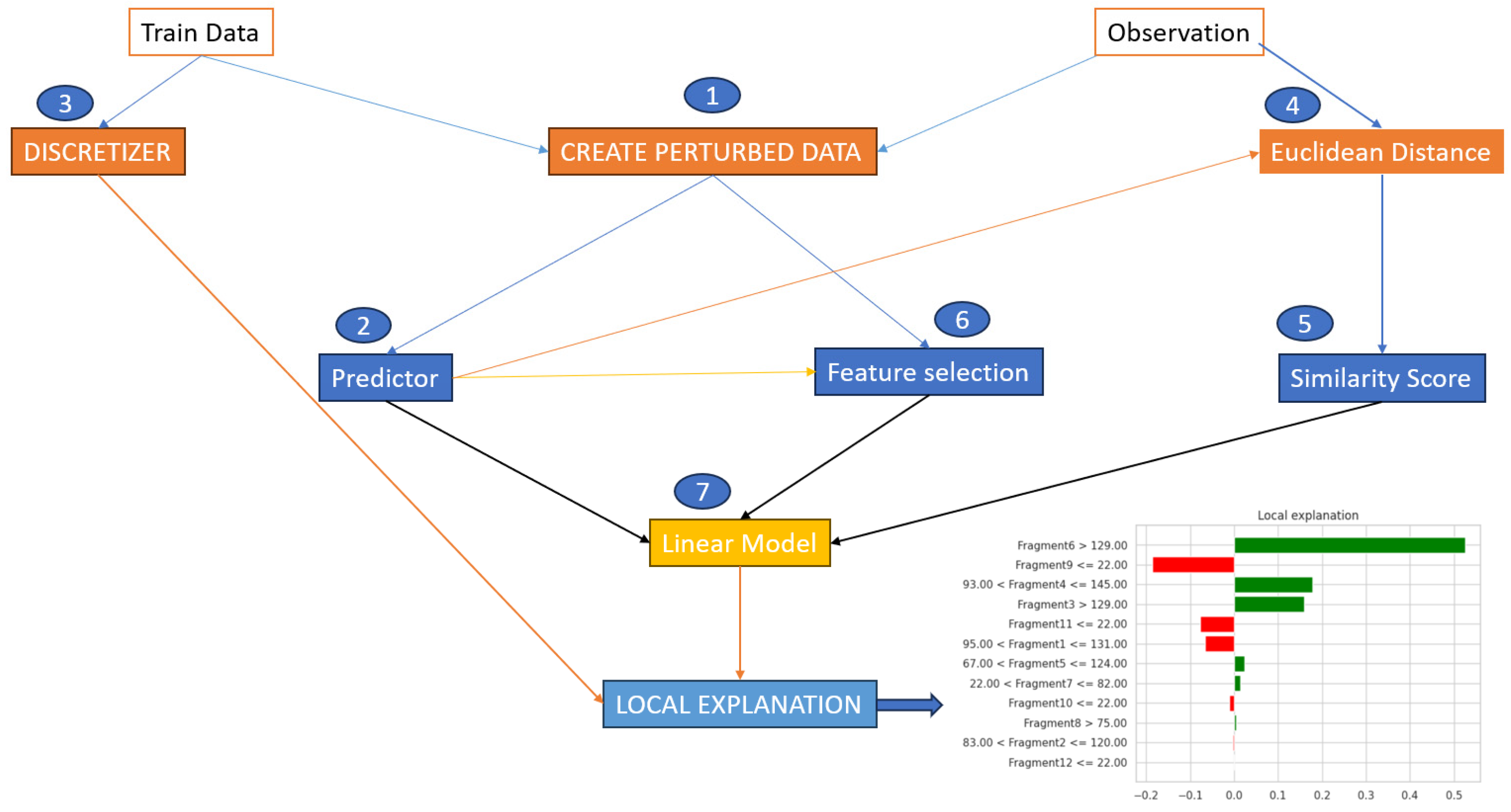This can be achieved by perturbing the instance, such as by adding noise or dropping features, to create new instances [11,12]. The selection of LIME as an explainability method in AI models, in preference to other techniques, hinges on the specific context and objectives of the application. LIME’s inherent model-agnostic nature makes it an appealing choice, as it can be seamlessly applied to a wide array of machine learning models, including complex black-box ones (which is illustrated in detail in Figure 4), without needing prior knowledge of the model’s architecture. Additionally, LIME specializes in providing localized explanations for individual predictions, catering to scenarios where understanding the rationale behind a single prediction holds more significance than explaining the entire model’s behavior. This becomes especially beneficial in applications where high-stakes decisions rely on individual instances, as it allows for pinpointed insights into why a specific prediction was made. Furthermore, the simplicity of LIME-generated explanations, which approximate intricate models with more interpretable ones, offers clarity and ease of understanding, which can be pivotal in scenarios where stakeholders and end-users require straightforward, human-intuitive explanations. On the other hand, the choice of LIME is also influenced by its transparency, as it reveals the most influential features behind a given prediction. This feature is vital in domains like healthcare and finance, where comprehending the impact of different input variables is of paramount importance. LIME is instrumental in error detection, enabling the identification of errors and biases in AI models, a crucial step towards ensuring fairness and accuracy. Moreover, in applications where human experts are actively involved in the decision-making process and need to both understand and potentially correct model predictions, LIME’s capacity to generate localized explanations fosters effective collaboration between human expertise and AI capabilities. Lastly, LIME helps to meet regulatory requirements that demand explanations for AI model decisions, making it a prudent choice for compliance in heavily regulated sectors.

Nevertheless, the selection of the most suitable explainability method should always be contingent on the specific use case, the nature of the AI model, and the unique needs of the stakeholders, as other methods like SHAP, integrated gradients, and decision trees may offer distinct advantages in differing contexts. Evaluating the strengths and limitations of each approach is key to ensuring that the chosen method aligns with the interpretability prerequisites of the application at hand. For our case, after several analyses related to these techniques, we came to the conclusion that the most advantages are provided by the use of LIME. This method excels in providing localized explanations. It focuses on explaining individual predictions rather than the global behavior of the model.

This granularity is especially valuable in situations where understanding the rationale behind specific predictions is more important than having a holistic view of the model’s behavior. For instance, in healthcare, it can offer insights into why a particular diagnosis was made, which can be vital for both medical professionals and patients. After we achieved this, the training of an interpretable model followed, in this case a decision tree using the newly created dataset. This model should approximate the behavior of the black-box model in the local region around the instance we want to explain. Calculating the feature importance scores for the prediction by analyzing the coefficients or decision paths of the interpretable model is the next step. These feature importance scores explain how each feature contributed to the prediction [13]. The last step is to use the feature importance scores to create an explanation for the prediction. This explanation can be in the form of a visual or textual description that highlights the most important features and their contributions to the prediction. This can help us to better understand the dataset and to improve the performance of the black-box model. We assume that the perturbed samples are generated by perturbing the input instance x using some perturbation method. The kernel fn is a function that computes a similarity score between two data points. The num features parameter specifies the number of features to select in the local linear model [14].

Specifically, the application of the LIME algorithm consists of the following computations: (1) Generate new perturbed samples by applying a perturbation method to the input instance x. (2) Compute kernel weights for each perturbed sample using the kernel function. (3) Train a local linear model using the perturbed samples, kernel weights, and labels for the black-box model’s predictions. (4) Compute feature importance weights using the local linear model. (5) Generate an explanation of the black-box model’s prediction for the input instance x using the local linear model and feature importance weights.

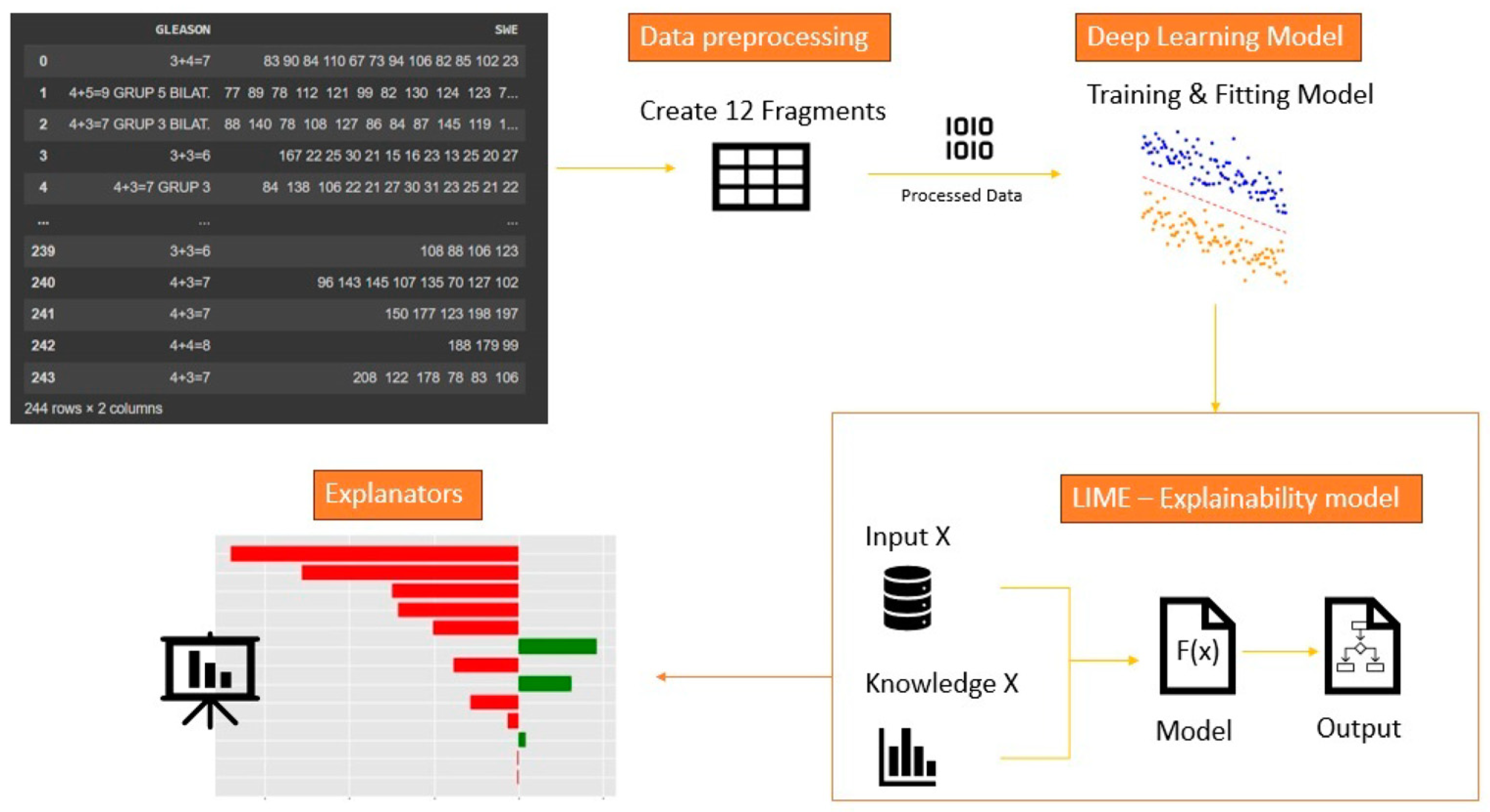
We trained a four-layer-deep neural network, and we evaluated the performance of the model using fourfold cross-validation with the task of binary classification. We designed from scratch a six-layer-deep neural network for the urology dataset using, again, a fourfold cross-validation for the multi-class case. Here, we included an extra step, namely, the encoding of the data. The values that were retained in y were encoded as a list of three binary values using one-hot encoding. This is a widely used technique in data preprocessing that plays a crucial role in converting categorical data into a numerical format suitable for machine learning algorithms. This technique works by taking categorical features, which are often represented as strings or labels, and transforming them into binary vectors. Each category is assigned a unique binary column, and the presence of a particular category is denoted by a ‘1’ in its respective column, while all other columns hold ‘0 s’. One-hot encoding ensures that categorical data does not introduce any ordinal relationship or magnitude, thus making it suitable for models that require numerical input. This method is advantageous in classification and regression as it helps models to interpret and utilize categorical information effectively. We used this in order to be able to apply the classification algorithms for later extraction, with the help of the LIME explainability method the characteristics that were relevant in predicting urological malignancies.

The classifier we used was a fully connected dense neural network for both datasets, because we aimed to use the same neural network architecture for both datasets. After training the model, we obtained a prediction accuracy of approximately 60% for the characteristics of the dataset. We aimed to visualize the impact and the way the developed model behaved with different data of different volumes of information and of different classes. After reaching this accuracy level, we were able to observe the relevant and least relevant characteristics for the prediction of thoracic diseases.

The architecture of the model was developed until we were able to extract the relevant characteristics and interpret the result as in the Figure 5:

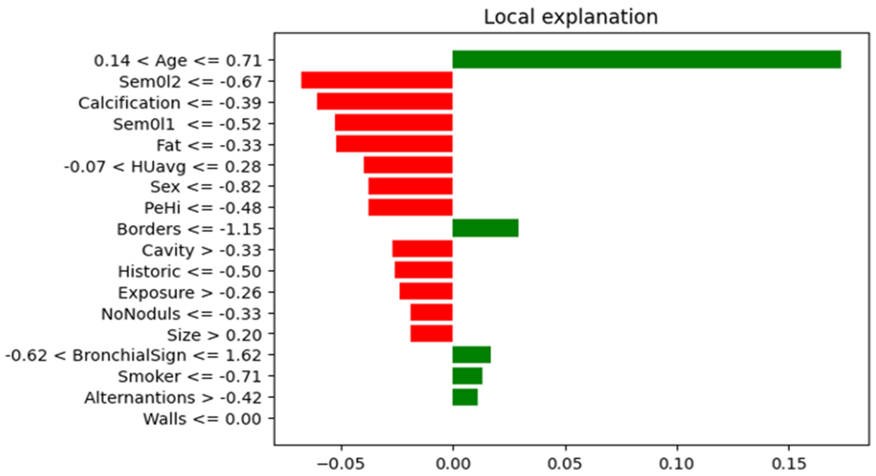
In Figure 6, it can be observed that the most important characteristics for the thoracic dataset were: Age, Borders, BronchicalSign, Smoker, Alternations, and Walls.

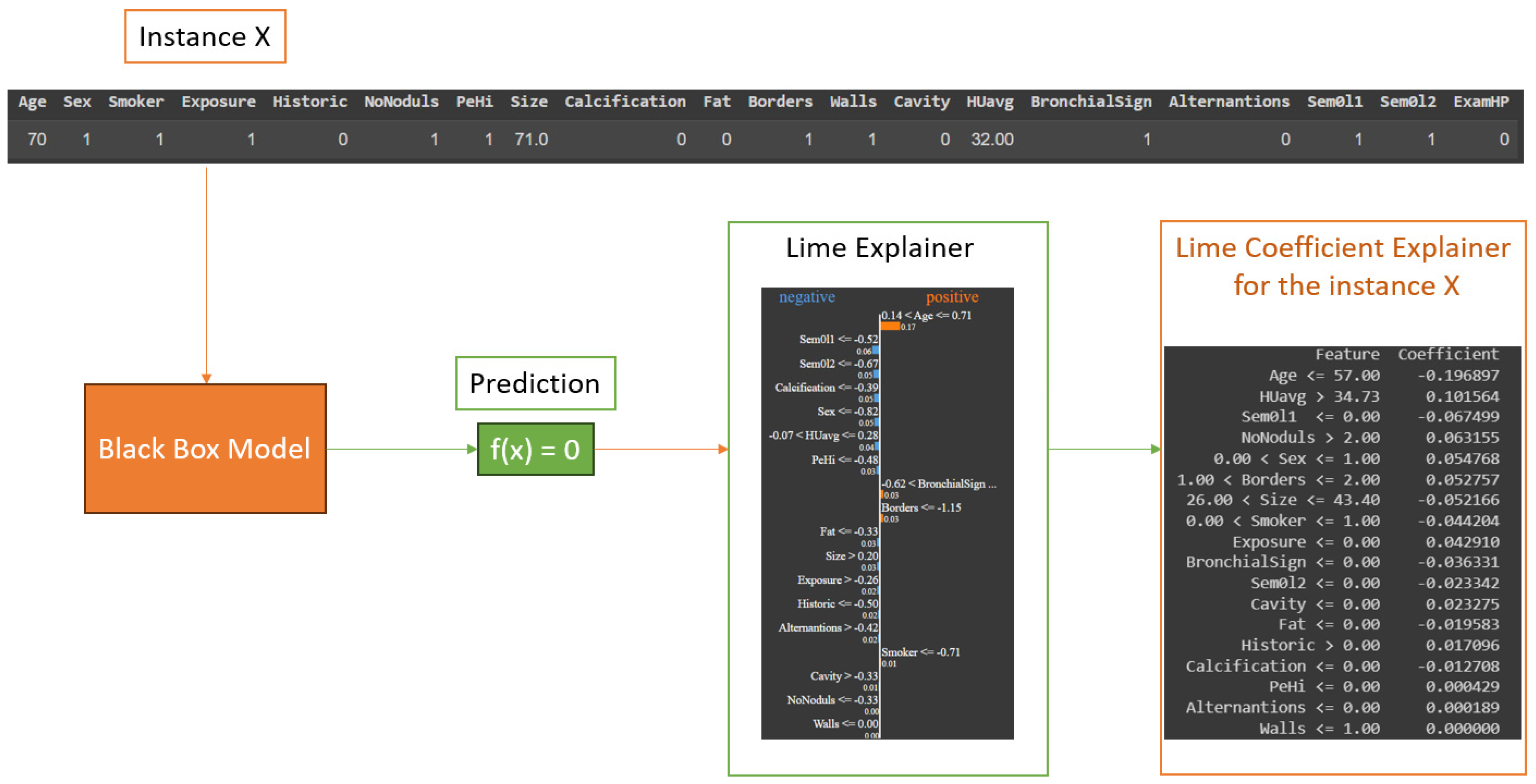
Although we have observed and extracted the most important characteristics from the thoracic dataset, it is also important to specify how the LIME algorithm works to reach the result presented above. For this, we chose to represent in Figure 7 the entire process that each instance in our dataset underwent. This should be coupled with the process from Figure 4, in which we explained in detail the black box process and what exactly occurred at that point. The steps for each instance were as follows: take instance X, apply each point from Figure 4 in the specified order, and check the obtained result. If the prediction was correct or not, then, we analyzed the obtained result and collected the conclusions.

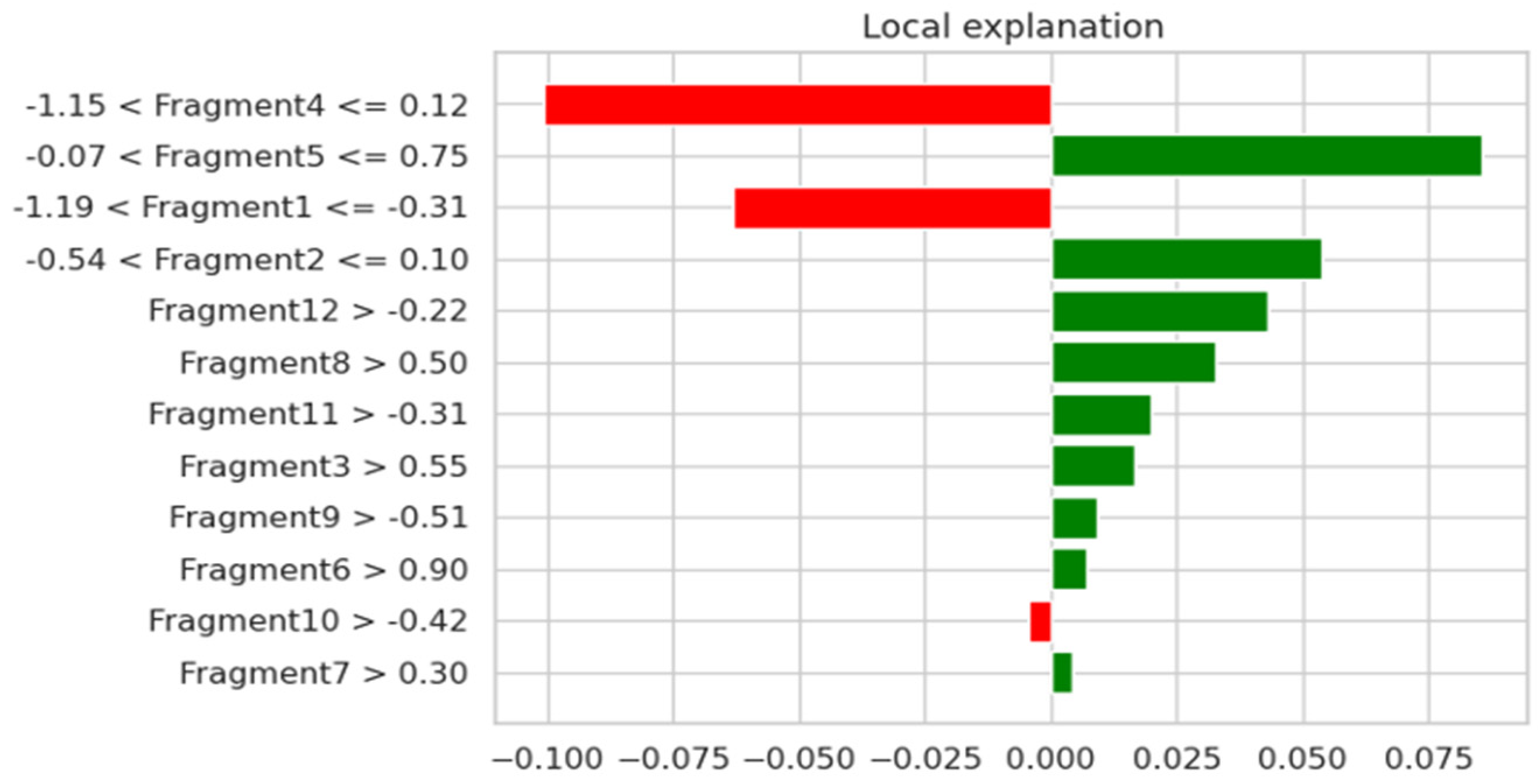
For the urology dataset, the most relevant characteristics were: Fragment3, Fragment5, Fragment6, Fragment7, Fragment8, Fragment9, Fragment11, and Fragment12, which are illustrated in Figure 8. By using the attention mechanism, we focused our deep neural network encoder on the characteristics listed above in order to obtain a prediction as relevant as possible for the considered dataset. If we were to analyze the result obtained only after applying the LIME explainability method, we could support the fact that the result was slightly different. In the case of the thoracic dataset, out of 18 independent characteristics, the model identified only 5 as relevant for the dataset, while for the urologic dataset, we obtained many more important characteristics. More precisely, for the urology dataset, we noticed that there were nine relevant features.

In this study, to design the model, we used four and six layers of the types Dense and BatchNormalization. We chose a value of seven as the input shape for the thoracic dataset and eight for urology dataset, because we excluded the last feature, and the activation functions used were ReLU and Sigmoid. The input shape value for a Dense layer in a neural network depends on the specific architecture and the preceding layers in the network. In a Dense layer, each neuron is connected to every neuron in the previous layer, which means that the input shape of the Dense layer should match the output shape of the preceding layer. To optimize the model, we used Adam optimized, and the number of epochs chosen was 250. The number of 250 epochs was chosen because we noticed that, once we reached this epoch, the model was trained better and the result was a very good one for datasets with small volumes of information. We attempted to increase the number of epochs, but in doing so, we caused overfitting, so we chose to use a volume of 250 epochs. The main purpose of a dense layer is to learn complex relationships between the input and output data [15]. The layer applies a linear transformation to the input data, followed by a non-linear activation function. The output of the layer can then be fed into another dense layer or a different type of layer in the neural network. The number of neurons in a dense layer is a hyperparameter that can be tuned to optimize the performance of the neural network [16]. Increasing the number of neurons in the layer can increase the capacity of the network to learn complex data.

ReLU stands for rectified linear unit and is a commonly used activation function in neural networks. It is a simple and efficient non-linear activation function that is widely used in deep learning models. The ReLU activation function applies the rectification operation to the input, which simply sets any negative values to zero and leaves the positive values unchanged [17].

Mathematically, the function can be expressed as:

f(x) = max(0, x), where x is the input to the function.

(1)

The sigmoid function is a popular activation function used in artificial neural networks. It is a smooth, S-shaped function that maps any real-valued number to a value between 0 and 1. The sigmoid function is defined mathematically as:

f(x) = 1/(1 + ex), where x is the input to the function.

(2)

The sigmoid function is often used in the output layer of a neural network to produce a probability value that can be interpreted as the likelihood of a certain class [18]. The main idea behind Adam is to adapt the learning rate for each weight in the neural network based on the average of the first and second moments of the gradients. The first moment is the mean of the gradients, while the second moment is the variance of the gradients. The algorithm calculates the adaptive learning rates for each weight in the network based on the moving averages of the first and second moments of the gradients [19]. These moving averages are computed using exponential decay rates, which allows the algorithm to give more weight to recent gradients and less weight to older ones [20]. We chose to use such a large number of epochs because the dataset was very small, and, thus, we wanted to learn more about the model to correctly predict the result. Thus, based on the combination of LIME and the Attention mechanism, our newly developed algorithm, to be used to increase the prediction accuracy, could be summarized in Algorithm 1:

Algorithm 1: The features attention coupling algorithm
1.	Input: clinical features dataset;
2.	Output: features-attention retrained neural network;
3.	Specify the architecture of the network;
4.	Perform k-fold cross-validation to evaluate the network;
5.	Call the LIME explainability method on the network;
6.	Analyze the explanations from LIME and select the relevant features;
7.	Activate the attention mechanism in the network;
8.	Modify the network based on insights gained and retrain the network;
9.	Return improved network.

5. Medical Discussion

After training the dataset that included only the characteristics with positive impacts that were relevant to our analysis, we managed to increase its accuracy by 20%, compared to the instance when we used the entire dataset. The accuracy value obtained following the use of the LIME method and the application of the attention mechanism on both datasets was approximately 80%.

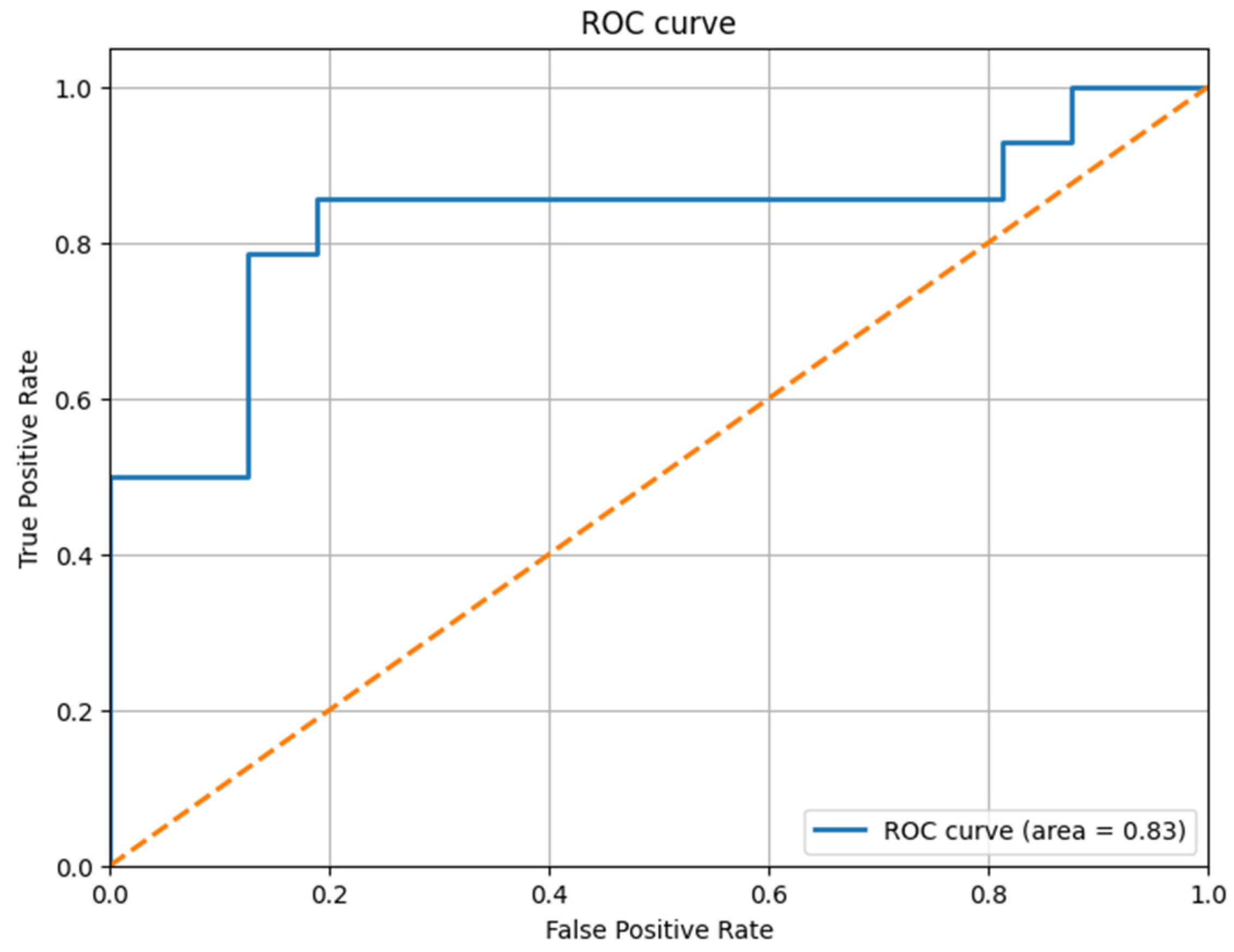
All the obtained results are illustrated with the help of the confusion matrix and the ROC curve, illustrated in Figure 9 for the thoracic dataset and in Figure 10 and Figure 11 for the urology dataset. We noticed that, after the prediction, the obtained ROC curve was ascending and quite linear for such a small volume of data (see Figure 9). Therefore, we confirmed the assumption that, by extracting only the relevant information, the model can be trained more correctly, and we can obtain a better result that is closer to reality. We present the results before and after using our method for the thoracic dataset in

Table 2. Performance metrics for the thoracic case (binary classification).

	The Result before Using the Developed Method	The Result after Using the Developed Method
Accuracy	60.48%	79.38%
Sensitivity	50.1%	57.07%
Specificity	69.19%	99.98%

.

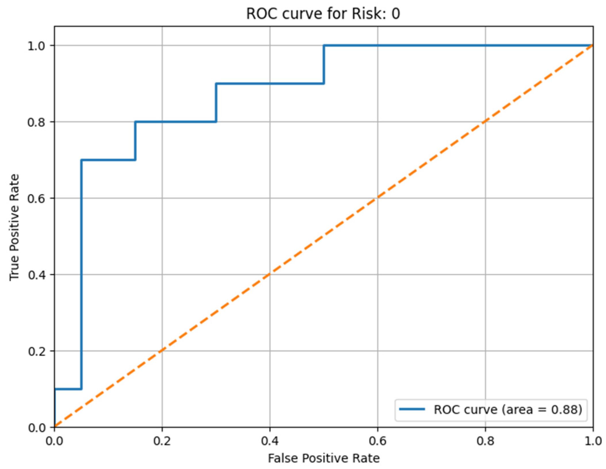
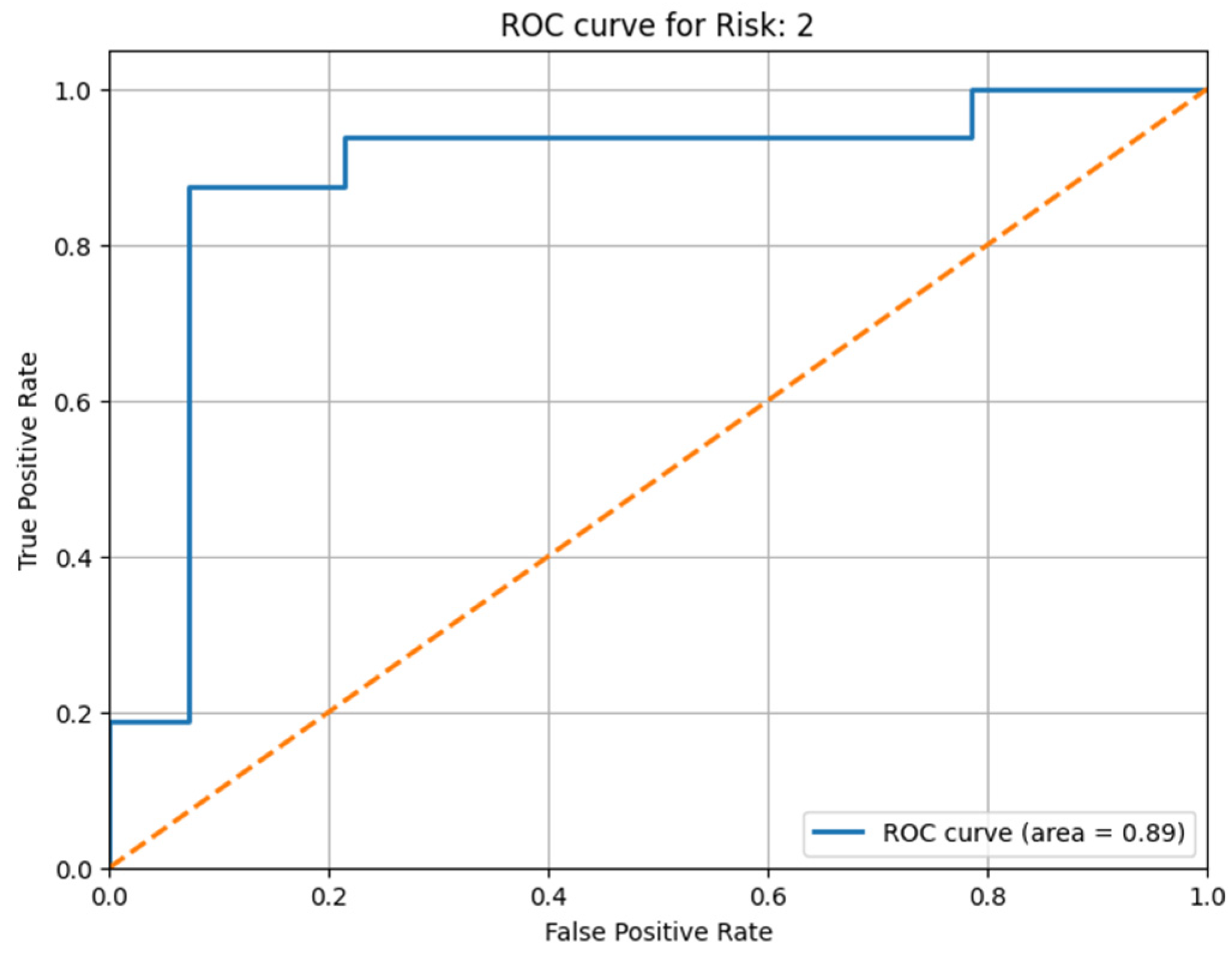
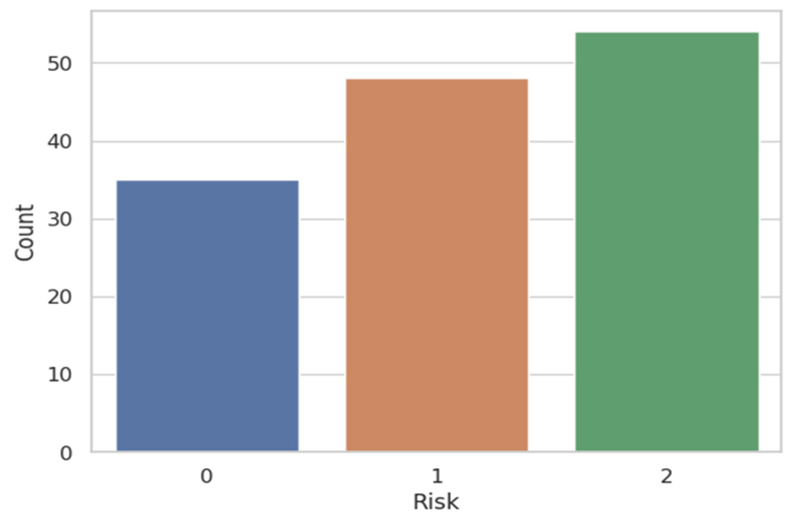
For the multi-class case, the result was even better. We illustrate in Figure 10 and Figure 11 the result obtained after applying the attention mechanism to the urology prostate cancer dataset. We chose to illustrate the results for Risk 0 and for Risk 2, because from Figure 2, we can observe that approximately 35 patients were classified with Risk 0 and over 50 patients with Risk 2. Patients with Risk 1 were under 50, so they fell in the middle as a volume of patients with intermediate risk of prostate cancer. To extend the ROC-AUC performance metric to multi-class classification for Risk 0 and Risk 2, which are the most interesting clinical cases, we have used a One-vs.-Rest (OvR) approach. Therefore, a separate ROC curve was plotted for each class against all other classes, effectively treating the multi-class problem as a multiple binary classification problem. Following the obtained result, we can state that the developed model worked very well on the multi-class case and on a larger volume of information.

We illustrate the result for the urology dataset in

Table 3. Performance metrics for the urology dataset (multi-class classification).

	The Result before Using the Developed Method	The Result after Using the Developed Method
Accuracy	63.81%	78.18%
Sensitivity	50.01%	54.55%
Specificity	75.76%	99.97%

and represent the values of accuracy, sensitivity, and specificity before and after using our technique.

6. Conclusions

By using the LIME explainability method for the purpose of extracting the relevant features and applying the features attention mechanism to them, we managed to increase the accuracy of the final model by approximately 20% from 60% in the first run to above 80% after the explainability-attention refinement. Thus, we highlighted the importance of extracting only the relevant features from the initial dataset. We managed to apply this method to obtain good predictions, even if the size of the dataset was small, with only 100 real patients in the first dataset and 138 real patients in the second dataset participating in this study.

We compared our novel model, including dense classification layers, with the standard deep neural network that is embedded into it. The results are shown in Table 2 and Table 3, where the performance metrics before using the developed method are shown along with the ones computed for the dense neural network embedded in our model. There were two significant improvements over the standard deep learning approaches. One is based on the application of LIME to emphasize the feature importance, and the second is to use this information as a feedback signal for the attention mechanism.

Initially, the model was designed for a small dataset; later, it was tested on a dataset with a larger volume of information, as well as in the multi-class case, where it behaved very well.

Small datasets have unique characteristics and constraints that significantly influence the choice of methods and tools used for analysis and modeling. For instance, in small datasets, there is a higher risk of overfitting when using complex models, as these models might adapt too closely to the limited data available, failing to generalize well to new, unseen data.

At the same time, as a final conclusion, we would like to specify the fact that we were not focused on the volume of the dataset, but whether the developed model would be appropriate or bring a positive contribution to automatic learning. We aimed to analyze the performance of the model and to check whether, by using it, we will be able to improve the predictions. The fact that we followed two sets of data from the clinical field, but from different areas of medicine, furthermore proves the versability and the flexibility of the method in executing different tasks, e.g., binary and multi-class classification.