Contact Force Surrogate Model and Its Application in Pantograph–Catenary Parameter Optimization

Abstract

The significant increase in the speed of high-speed trains has made the optimization of pantograph–catenary parameters aimed at improving current collection quality become one of the key issues that urgently need to be addressed. In this paper, a method and solutions are proposed for optimizing multiple pantograph–catenary parameters, taking into account the speed levels and engineering feasibility, for pantograph–catenary systems that contain dozens of parameters and exhibit strong nonlinear coupling characteristics. Firstly, a surrogate model capable of accurately predicting the standard deviation of contact force based on speed and 14 pantograph–catenary parameters was constructed by using the pantograph–catenary finite element model and feedforward neural network. Secondly, sensitivity analysis and rating of the pantograph–catenary parameters under different speeds were conducted using the variance-based method and the surrogate model. Finally, by combining the sensitivity analysis results and the Selective Crow Search Algorithm, joint optimization of 10 combinations of the pantograph–catenary parameters across the entire speed range was performed, providing efficient pantograph–catenary parameter optimization solutions for various engineering conditions.

1. Introduction

The problem of the pantograph–catenary relationship becomes more prominent, and the design of pantograph–catenary faces more technical challenges with further increases in train speed [1,2,3]. The contact force between the panhead strip and the contact wire is a direct reflection of the pantograph–catenary interaction. The mean contact force and the standard deviation of contact force (SDCF) are the main evaluation indicators of current collection quality [4,5,6]. A good pantograph–catenary performance refers to minimizing the SDCF as much as possible while satisfying the requirements for the average contact force. Therefore, to improve the current collection quality, it is common to optimize the pantograph–catenary parameters to minimize the objective function, i.e., the SDCF.

To reduce the computational complexity and improve optimization efficiency in parameter optimization, it is effective to conduct a sensitivity analysis of the SDCF with respect to pantograph–catenary parameters first. For example, the first-order sensitivities of nine pantograph parameters for a GPU pantograph and a simple suspension catenary at 100~400 km/h [7], and a DSA380 pantograph and a stitched suspension catenary at 350 km/h [8]; the first-order sensitivities of four catenary parameters and nine pantograph parameters for a simple suspension catenary at 90~150 km/h [9]; the first- and second-order sensitivities of four catenary parameters for a CX-type pantograph and a simple suspension catenary at 300 km/h [10]. Existing reports indicate that the sensitivity to the equivalent mass of the panhead vertical vibration is the highest among the pantograph parameters, while other parameters show significant differences in sensitivity rating. The sensitivities to the span and contact wire density are higher than those to the pantograph parameters, and the sensitivities to parameters such as the pre-tensions of the contact wire and messenger wire are relatively high among the catenary parameters. However, differences in the sensitivity analysis results of pantograph–catenary parameters arise from variations in the operating speed, catenary type, and baseline parameters considered in different reports. Additionally, as pantograph–catenary parameters involve multiple parameters with strong nonlinear coupling, it is essential to investigate higher-order or total sensitivities that characterize the interaction effects between pantograph–catenary parameters.

Typically, the objective of the joint optimization of pantograph–catenary parameters is to minimize the SDCF. In terms of single-parameter optimization, the control variable method can be used effectively [11]. In terms of multi-parameter optimization, the robust design technique [12] and optimization algorithms [13,14] can be used to search for the optimal solutions. As for optimization algorithms, the optimization iteration process involves a significant number of dynamic calculations for pantograph–catenary samples. The more parameters to be optimized, the greater the number of samples required. Classical pantograph–catenary finite element models consume approximately 10 core hours per sample, resulting in substantial computational costs. To mitigate computational resource consumption, it is a viable approach to use the pantograph–catenary finite element method to precompute a sufficient number of pantograph–catenary interaction samples and then employ data fitting or machine learning algorithms to establish the functional relationship between the SDCF and pantograph–catenary parameters. This approach can significantly alleviate the computational burden in optimization iterations. Based on a multi-layer feedforward deep residual neural network, a surrogate model of the SDCF with respect to 11 catenary parameters was established [15]. Based on the response surface method [16] or the Pseudo-monte Carlo method [17], a quadratic function of the SDCF on several pantograph parameters could be established, and then the parameters’ optimal solution could be obtained by solving the minimum value of the function. By using the backpropagation algorithm [18] or the Selective Crow Search Algorithm to train radial basis function neural networks [19], surrogate models of the SDCF with respect to six pantograph dynamic parameters were established, which were then used for pantograph parameter optimization, combined with optimization algorithms.

The paper is organized as follows: In Section 2, a surrogate model capable of accurately predicting the SDCF based on operating speed and 14 pantograph–catenary parameters was constructed using a combination of a feedforward neural network and a validated pantograph–catenary finite element model. This surrogate model is intended to replace pantograph–catenary dynamic finite element calculations. Next, with the surrogate model and the variance-based method, both the first-order and total sensitivities of pantograph–catenary parameters were calculated in Section 3, considering factors such as speed and parameters interaction effects. Subsequently, based on the sensitivity analysis results, the surrogate model, and the Selective Crow Search Algorithm, joint optimization of 10 pantograph–catenary parameter combinations for speeds ranging from 250 to 450 km/h was performed in Section 4, providing pantograph–catenary parameter optimization recommendations across the entire speed range. Finally, Section 5 presents the conclusions.

2. Surrogate Model Training by Feedforward Neural Network

2.1. Design of Data Sets

The input parameters consisted of the speed (v), nine pantograph parameters, and five catenary parameters, i.e., X = {m₃, m₂, m₁, k₃, k₂, k₁, c₃, c₂, c₁, T_c, T_m, A_c, A_m, L, v}^T. The output parameter was the SDCF at a low-pass filtering frequency of 20 Hz or 40 Hz. The value of each input parameter X_r(r = 1, 2, …, 15) was determined according to engineering practice (

Table 1. Value of input parameters.

Input Parameters	Unit	Value Range	Value Interval	Reference Value
v	km/h	[250, 380]	2	/
		(380, 450]	1
m3	kg	[5, 11]	0.02	7.94
m2	kg	[5, 20]	0.05	8.22
m1	kg	[3, 20]	0.05	5.9
k3	N/m	[4000, 14,000]	50	6650
k2	N/m	[8000, 20,000]	80	13,181
k1	N/m	[0, 200]	1	74
c3	N·s/m	[0, 100]	0.5	85.31
c2	N·s/m	[0, 50]	0.5	11.9
c1	N·s/m	[10, 240]	1	67.41
Tc	kN	[27, 40]	1	30
Tm	kN	[19, 25]	1	21
Ac	mm2	[121, 180]	29.5	151
Am	mm2	[93.27, 147.12]	26.93	116.99
L	m	[48, 65]	1	55

). Among them, m_i, k_i, and c_i are the equivalent mass, stiffness, and damp, respectively, and i = 1, 2, 3 represent the mass point of the frame rotation, upper frame vertical vibration, and panhead vertical vibration; T_c and T_m are the tension of contact wire and messenger wire, A_c and A_m are the cross-section area of contact wire and messenger wire, and L is the span length.

The steps for data set design are as follows: First, draw 12,000 samples by using the Latin hypercube sampling method [20]. Secondly, the time domain curves of contact force for the above 12,000 samples were obtained using the pantograph–catenary finite element method [21], and the lifting force exerted on m₁ was adjusted during calculation to ensure the deviation between the average contact force and the upper limit [6] was lower than 0.5 N. Based on those time domain curves after low-pass filtering at 20 Hz or 40 Hz, the theoretical values of the SDCF could be calculated, and databases of the SDCFs at the two low-pass filtering frequencies were constructed. Finally, the training set and the validation set were divided from the data set based on the hold-out method, and the test set was composed of the remaining examples. The ratio of the sample size of the three sets was 8:1:1. When dividing the training set and validation set, stratified sampling was used to maintain the consistency of the data distribution and avoid introducing additional bias and affecting the generalization ability of the surrogate model due to the data dividing.

2.2. Training of Surrogate Model

Map X_r of all samples of the three sets to the interval [−1, 1] and the processed input parameter value can be obtained as

$$x_r=\frac{2\left(X_r-X_{r\min }\right)}{X_{r\max }-X_{r\min }}-1,$$

(1)

where X_rmin is the lower limit of X_r in the value space, and X_rmax is the upper limit. Map σ to the interval [0, 1] and the processed output parameter value, i.e., $\left(\sigma -{\sigma }_{\min }\right)/\left({\sigma }_{\max }-{\sigma }_{\min }\right)$ can be obtained, where σ_min and σ_max are the minimum and maximum of σ for all examples.

A three-layer feedforward neural network (Figure 1a) was employed to construct a surrogate model that predicts the SDCF based on pantograph–catenary parameters. The r-th neuron x_r in the input layer is connected to the first hidden layer's h-th neuron with a connection weight ω_rh. ${\displaystyle \sum _{r=1}^{15}{\omega }_{rh}{x}_r-{\theta }_h}$ is applied to a specific activation function to compute the output value of that neuron. Similarly, the output values from the previous hidden layer are transmitted to the next hidden layer through connection weights until the output value of the h-th neuron in the third hidden layer, b_h, is obtained. b_h is then transmitted to the output layer with a connection weight υ_h, and the output value of the output layer's neuron is calculated by applying ${\displaystyle \sum _{h=1}^{H_3}{\upsilon }_h{b}_h-\gamma }$ to an activation function. After denormalization, this yields the SDCF. Among them, H₁, H₂, and H₃ are the neuron numbers of the three hidden layers, θ_h is the threshold of the h-th neuron of the first hidden layer, and γ is the threshold of the output layer’s neuron. The neuron numbers and activation functions of hidden layers and output layers are shown in

Table 2. Hyper-parameter settings of neural network layer in surrogate model.

Neural Network Layer	Number of Neurons	Activation Function
1st hidden layer	20	tanh
2nd hidden layer	10	tanh
3rd hidden layer	5	sigmoid
output layer	1	relu

.

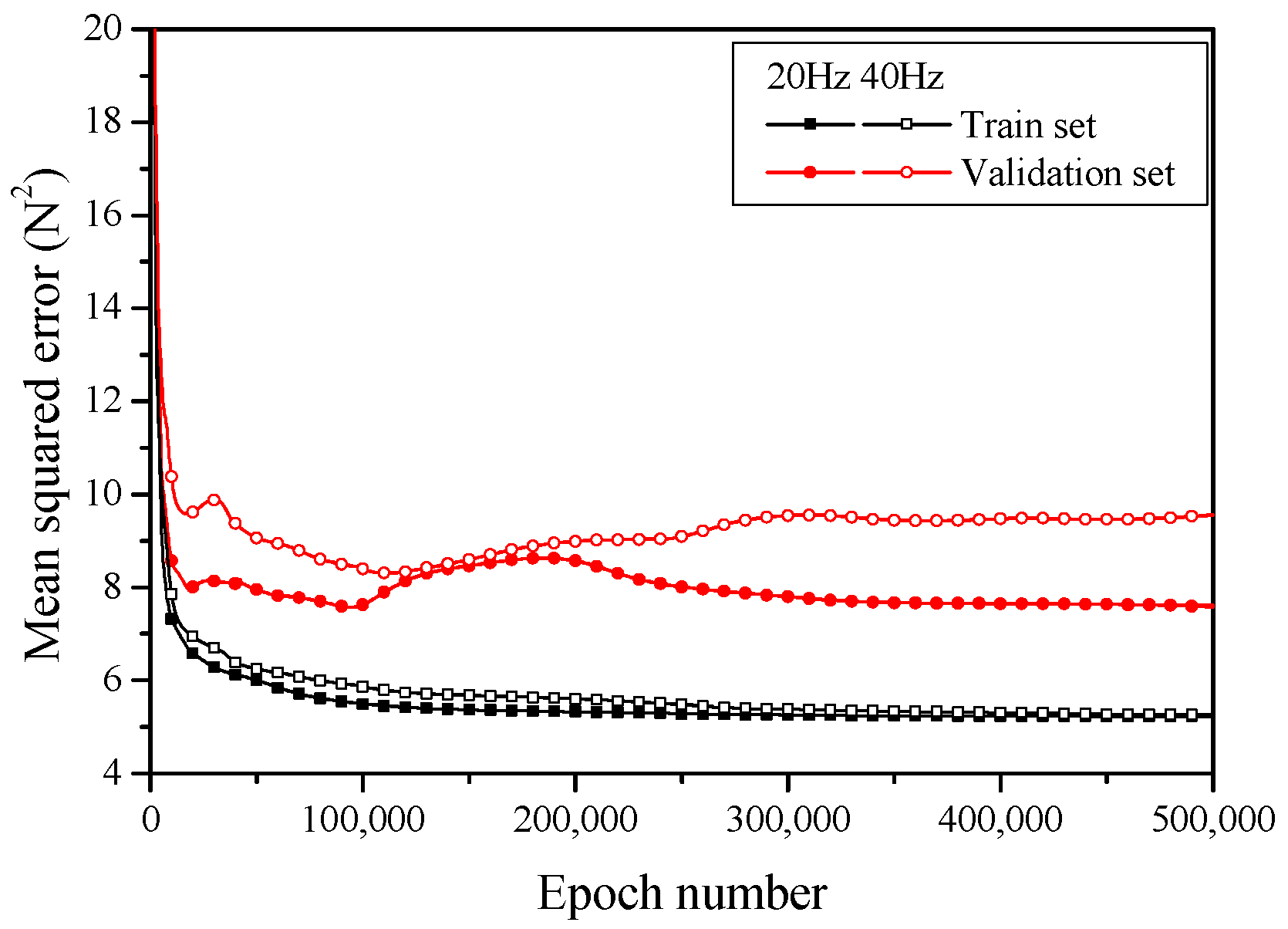
The training of the SDCF surrogate model was accomplished by taking the minimizing of the mean squared error on the training set as the objective, using the connection weights and thresholds for the hidden and output layers as the decision vectors, and employing Adam Optimizer to find the optimal solution. Firstly, the connection weights and thresholds were respectively initialized to a set of normally distributed random numbers with a mean of 0 and a standard deviation of 0.05. Following the Adam update rules, these weights and thresholds were updated, and the corresponding mean squared errors for the training and validation datasets were computed. This process iterated until the maximum of 500,000 iterations. The optimizer's learning rate was set for 0.0005, and each training batch consisted of 1024 samples. It could be observed that as the number of iterations increases, the mean squared errors for both the training and validation datasets tend to converge (Figure 2). Finally, to mitigate overfitting, according to early stopping [22], all connection weights and thresholds were set for the values when the mean squared error on the validation dataset was minimal.

2.3. Performance Measure of Surrogate Model

Calculate the predicted SDCF value, ${\widehat{\sigma }}_p$, for all samples in the test set. Using the error, ${\widehat{\sigma }}_p-{\sigma }_p$, the error distribution interval within 0.95 probability, the mean square error ${\displaystyle \sum _{p=1}^{1200}{\left({\widehat{\sigma }}_p-{\sigma }_p\right)}^2/1200}$, and the determination coefficient, $1-{\displaystyle \sum _{p=1}^{1200}{\left({\widehat{\sigma }}_p-{\sigma }_p\right)}^2}/{\displaystyle \sum _{p=1}^{1200}{\left({\sigma }_p-\overline{\sigma }\right)}^2}$, as evaluation indicators for the generalization ability of the surrogate model [23]. Among them, σ_p is the FEM calculated value of the SDCF, p = 1, 2, …, 1200, and $\overline{\sigma }$ is their average value.

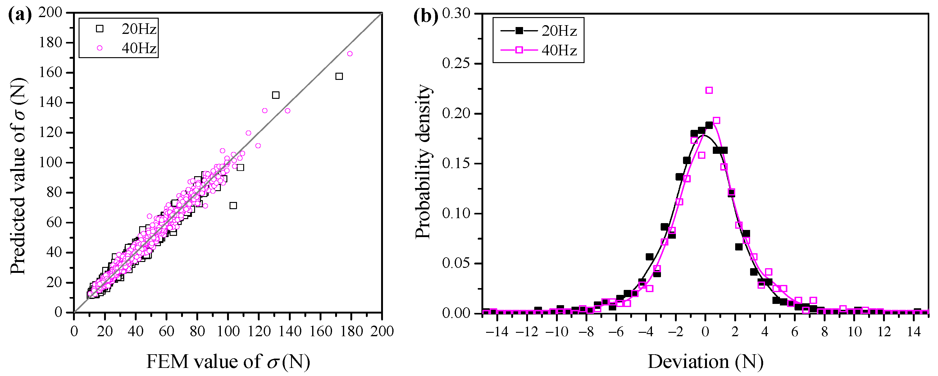
The error of the surrogate model obtained at a low-pass filtering frequency of 20 Hz or 40 Hz on the test set follows a normal distribution approximately (Figure 3). The error distribution intervals of 0.95 probability were about [$-$6.06, 5.11] N and [$-$5.67, 6.12] N, the mean squared errors were about 7.93 N² and 7.66 N², and the determination coefficients were about 0.971 and 0.982, respectively (

Table 3. Prediction errors of surrogate models on test set.

Cut-Off Frequency (Hz)	Error Interval within the Probability of 0.95 (N)	Mean Squared Error (N2)	Coefficient of Determination
20	[−6.06, 5.11]	7.93	0.971
40	[−5.67, 6.12]	7.66	0.982

). Obviously, the surrogate models obtained by the feedforward neural network have strong generalization ability, and the error between the predicted results and the FEM values is small.

3. Sensitivity Analysis of Pantograph–Catenary Parameters

3.1. Definition of Sensitivity

Sensitivity analysis is used to study the contribution of input parameter uncertainty to the uncertainty in the outputs of a model [24]. Sensitivity analysis can be divided into local sensitivity analysis and global sensitivity analysis, which focus on how input parameters affect output results both near their baseline values and within their entire range of values, respectively [25]. In this section, a variance-based method [26,27] is employed for sensitivity analysis of the SDCF with respect to pantograph–catenary parameters, and sensitivity indices are calculated. The higher the sensitivity indices of the input parameter, the greater the influence of the parameter on the SDCF.

At a specific operating speed, the input parameter x_r (r = 1, 2, …, 14) represents the aforementioned 14 pantograph–catenary parameters, and the output is the SDCF σ. The first-order, second-order, and total sensitivities of x_r are defined as follows:

$$S_r=V_{x_r}\left(E\left(\sigma \left|x_r\right.\right)\right)/V\left(\sigma \right),$$

(2)

$$S_{rt}=\left[V_{x_r{x}_t}\left(E\left(\sigma \left|x_r,x_t\right.\right)\right)-V_{x_r}\left(E\left(\sigma \left|x_r\right.\right)\right)-V_{x_t}\left(E\left(\sigma \left|x_t\right.\right)\right)\right]/V\left(\sigma \right),$$

(3)

$$S_r^{\mathrm{T}}=\left[V\left(Y\right)-V_{x_{~r}}\left(E\left(\sigma \left|x_{~r}\right.\right)\right)\right]/V\left(\sigma \right)=E_{x_{~r}}\left(V\left(\sigma \left|x_{~r}\right.\right)\right)/V\left(\sigma \right),$$

(4)

where S_r represents the impact of x_r on σ, S_rt represents the impact of the interaction effects between x_r and other input parameter x_t on σ, and S_r^T is the sum of the first-order sensitivity of x_r and all higher-order sensitivities. This is used to comprehensively measure the impact of the parameter itself and its interaction effects with other parameters on the model output. In the equation, r, t = 1, 2, …, 14, and t > r; x_~r denotes all input parameters except x_r; V(σ) is the total variance of σ when all input parameters vary arbitrarily within their ranges; $V_{x_r}\left(E\left(\sigma \left|x_r\right.\right)\right)$ is the average decrease in variance of σ, i.e., $V\left(\sigma \right)-E_{x_r}\left(V\left(\sigma \left|x_r\right.\right)\right)$, when x_r is fixed at all possible values within its range, while x_~r varies arbitrarily; and $E_{x_{~r}}\left(V\left(\sigma \left|x_{~r}\right.\right)\right)$ is the average variance of σ when x_~r is fixed at all possible values within their ranges, while x_r varies arbitrarily.

3.2. Sensitivity and Its Rating of Pantograph–Catenary Parameters

Due to the strong non-linearity of the surrogate model of the SDCF, it is difficult to calculate the variance terms in Equations (2)–(4) through integration. Therefore, with the Monte Carlo method, two independent sample matrices with the same sample size were used for estimation. For two low-pass filtering frequencies of 20 Hz and 40 Hz and five speeds, including 250, 300, 350, 400, and 450 km/h, sample sizes and input parameter values are predefined (Table 1). Based on the two previously designed sample matrices, each column is replaced one by one with the corresponding column from the other matrix, resulting in an increase of 29 times in the sample size [28]. Using bootstrapping with 10,000 times resampling to calculate the sensitivities of pantograph–catenary parameters and their 95% confidence intervals [29,30].

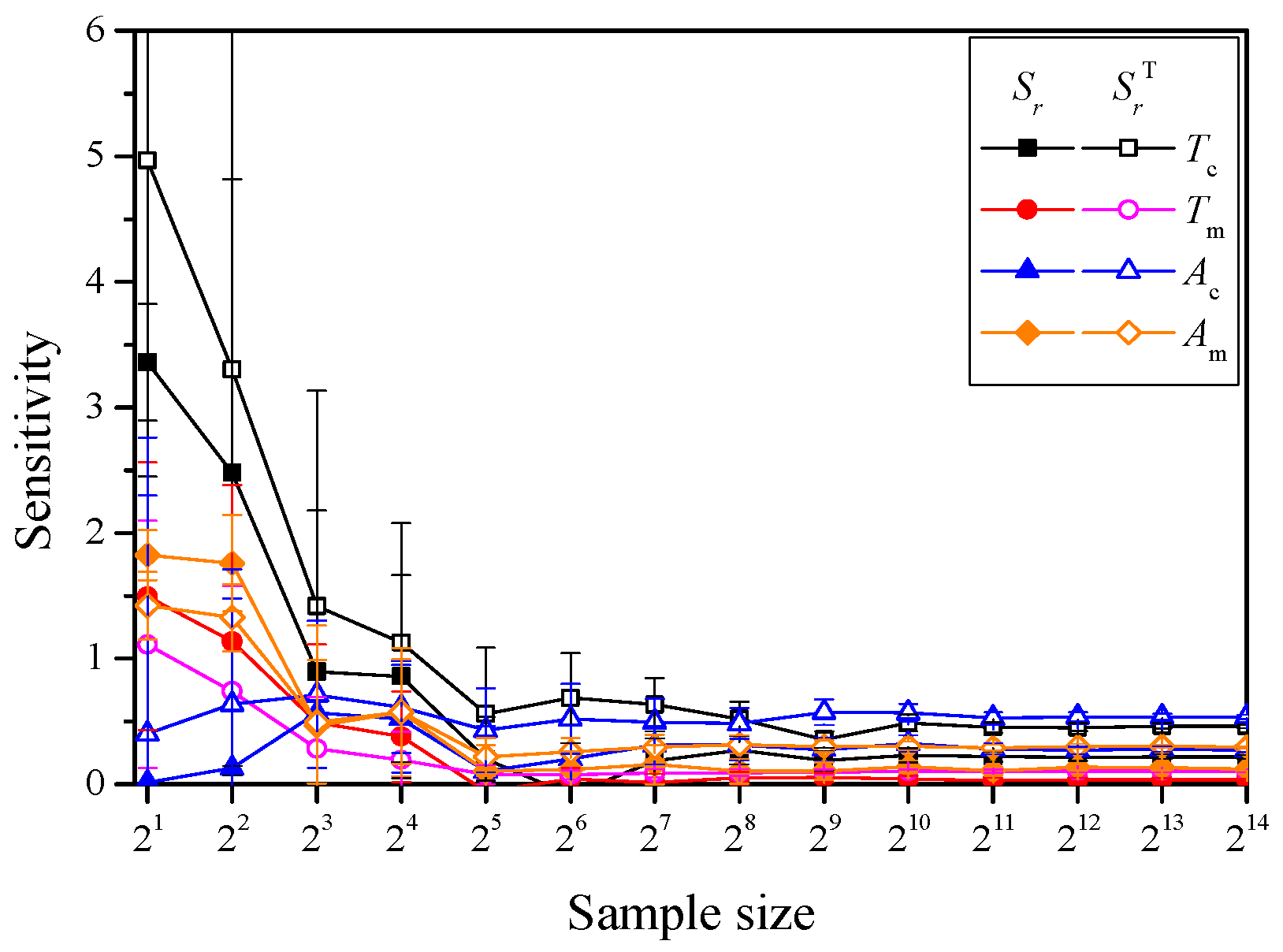
Statistical analysis of the first-order and total sensitivities of 14 pantograph–catenary parameters under five operating speeds and two low-pass filtering frequencies indicated that as the sample size increases, the sensitivities converge to specific values, and the 95% confidence intervals shrink, thus improving the accuracy and stability of sensitivities calculations (Figure 4). Considering the results for all operating conditions, a sample size of 2¹⁴ was chosen when the values of sensitivities reached a stable convergence.

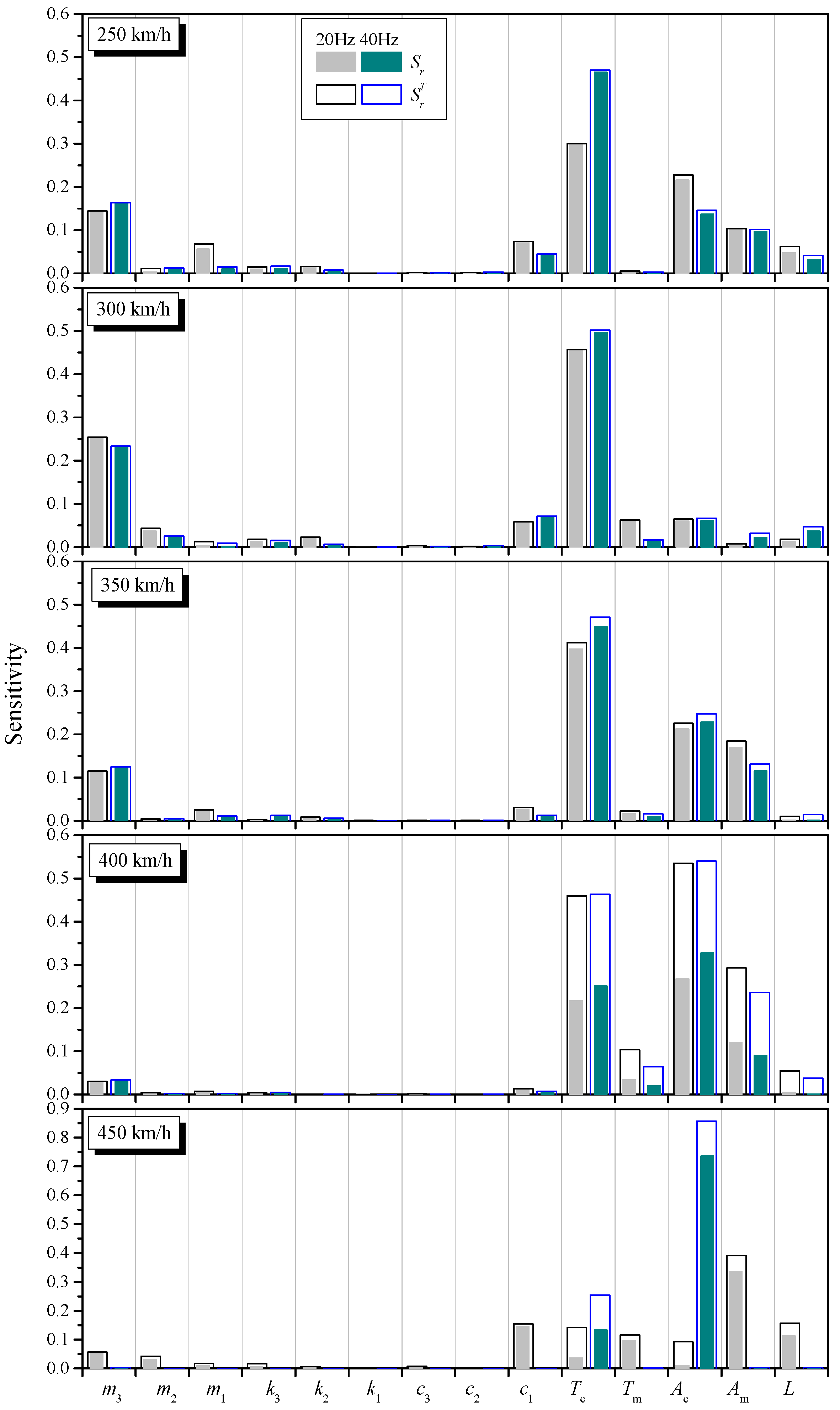
Figure 5 illustrates the first-order and total sensitivities of 14 pantograph–catenary parameters. The average sensitivity to each pantograph–catenary parameter under all operating conditions (Column 2 of

Table 4. Sensitivity rating of pantograph–catenary parameters.

Input Parameters	Average Value of Sensitivities	Rating
Tc	0.713	I
Ac	0.526
Am	0.254	II
m3	0.230
c1	0.091	III
L	0.069
Tm	0.067
m1	0.028	IV
m2	0.026
k3	0.017
k2	0.015
c3	0.003	V
c2	0.002
k1	0.001

) represents the level of the parameter’s impact on the SDCF. Using the k-means clustering algorithm from prototype clustering, the 14 average sensitivities are divided into five categories, thus providing a sensitivity rating for the pantograph–catenary parameters (Column 3 of Table 4). Among these, T_c and A_c are rated as Class I, as their impact on the SDCF is significantly higher than that of the other parameters. A_m and m₃ are rated as Class II; c₁, L, and T_m are rated as Class III; m₁, m₂, k₃, and k₂ are rated as Class IV; c₃, c_2, and k₁ are rated as Class V, and their impact on the SDCF can be ignored.

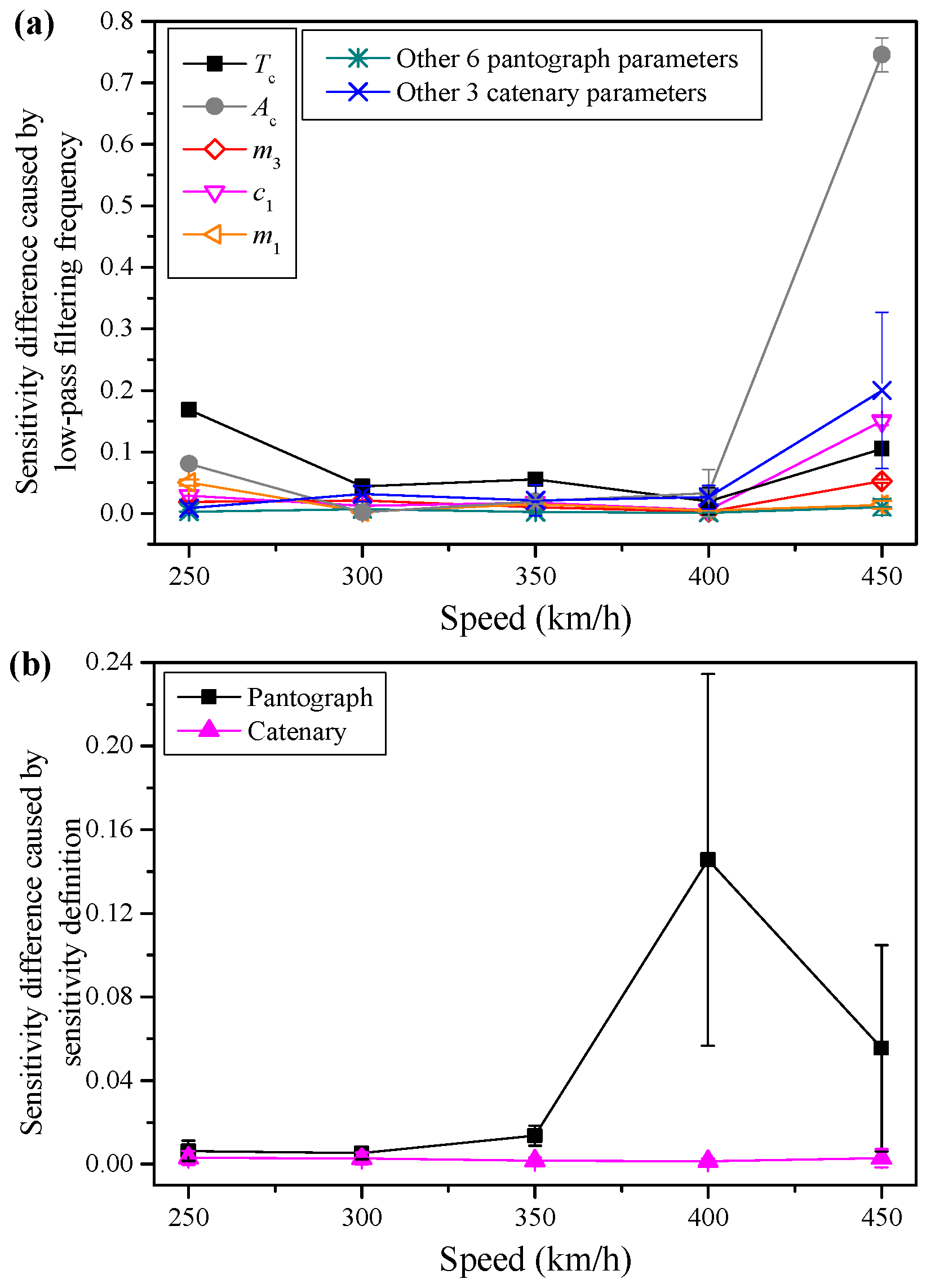
Changes in the low-pass filtering frequency of the contact force time-domain signal will only affect the sensitivities to certain pantograph–catenary parameters under specific operating conditions, which include T_c at all speeds, A_c and m₁ at 250 km/h, five catenary parameters, m₃ and c₁ at 450 km/h (Figure 6a). In other words, when the operating speed falls within the abovementioned speed ranges, altering the relevant pantograph–catenary parameters will result in a significant increase in the SDCF in the frequency range of 20–40 Hz. In all other cases, the impact of changing pantograph–catenary parameters on the SDCF in the frequency range of 20–40 Hz can be ignored.

At speeds of 400 km/h and above, there is a significant difference between the first-order and total sensitivities of the catenary parameters, indicating that at higher speeds, there is an additional increase in the coupling effects between the catenary parameters, which affects the SDCF (Figure 6b). In addition, for catenary parameters at 350 km/h and below, as well as for pantograph parameters at all speeds, sensitivity definitions have very little impact on sensitivities. In other words, the impact of coupling effects between parameters on the SDCF can be ignored.

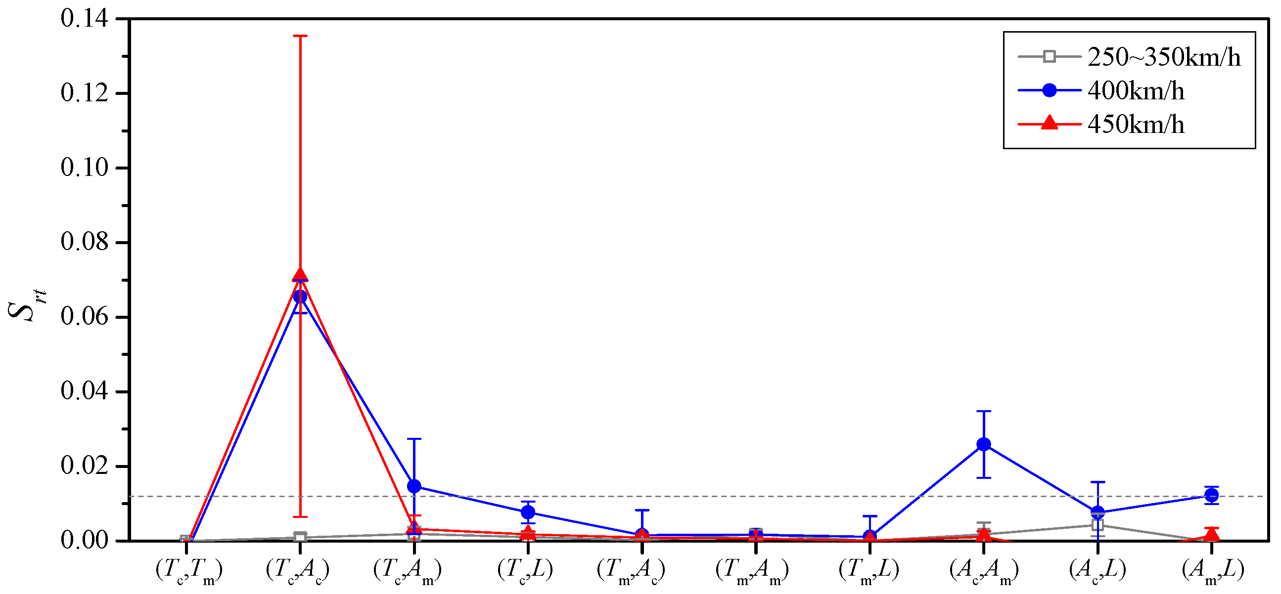
Figure 7 presents the second-order sensitivities of the catenary parameters. At 350 km/h and below, the second-order sensitivities to all catenary parameters are approximately zero. As the speed increases, the second-order sensitivities of (T_c, A_c) at 400 and 450 km/h and the second-order sensitivities of (T_c, A_m), (A_c, A_m) and (A_m, L) at 400 km/h are relatively high, while the second-order sensitivities in other scenarios are close to zero. This indicates that at medium and high speeds, the interaction effects between any two catenary parameters on the SDCF can be ignored, but at higher speeds, it is necessary to consider the interaction effects between T_c and A_c or A_m, A_m, and A_c or L on the SDCF.

4. Multi-Parameter Joint Optimization of Pantograph–Catenary

Using the Selective Crow Search Algorithm (SCSA) [19] with the optimization objective of minimizing the SDCF, the optimal solutions for 10 sets of decision vectors (

Table 5. Decision vectors composed of pantograph–catenary parameters.

Case	Pantograph Parameters	Catenary Parameters	Rating
1	m3, c1, m1, m2, k3, k2, c3, c2, k1	Tc, Ac, Am, L, Tm	I, II, III, IV, V
2	m3, c1, m1, m2, k3, k2	Tc, Ac, Am, L, Tm	I, II, III, IV
3	m3, c1	Tc, Ac, Am, L, Tm	I, II, III
4	m3	Tc, Ac, Am	I, II
5	/	Tc, Ac	I
6	/	Tc, Ac, Am, L, Tm	I, II, III
7	/	Tc, Ac, Am	I, II
8	m3, c1, m1, m2, k3, k2, c3, c2, k1	/	II, III, IV, V
9	m3, c1, m1, m2, k3, k2	/	II, III, IV
10	m3, c1	/	II, III

) and their corresponding SDCFs were iteratively searched (Figure 1c). These iterations were conducted under two low-pass filtering frequencies and five operating speeds. Specifically, Case 1 includes all pantograph–catenary parameters, while Case 2 to Case 5 successively reduce the number of pantograph–catenary parameters. Case 6 encompasses all catenary parameters, with Case 7 and Case 5 progressively reducing the number of catenary parameters. Case 8 represents all pantograph parameters, with Case 9 and Case 10 gradually reducing the number of pantograph parameters. To ensure the generalization ability of the optimization scheme, 100 random values were sampled for the other pantograph–catenary parameters outside the decision variables within their respective ranges using Latin Hypercube Sampling. Firstly, the relevant parameters of SCSA are set as follows: the maximum number of iterations is 500, the population size is 50, the flight length is 2, and the awareness probability is 0.1. The values of decision variables are shown in Table 1. Next, initialize the decision vector of all populations in the first generation and calculate the SDCF of all populations. Then, update the decision vector by the regulation of SCSA and calculate the corresponding SDCF repetitively until the number of iterations reaches the maximum value. Finally, the optimal solution is the decision vector with the smallest SDCF. The SDCF of the samples during the iteration process was computed using the surrogate model from Section 2. 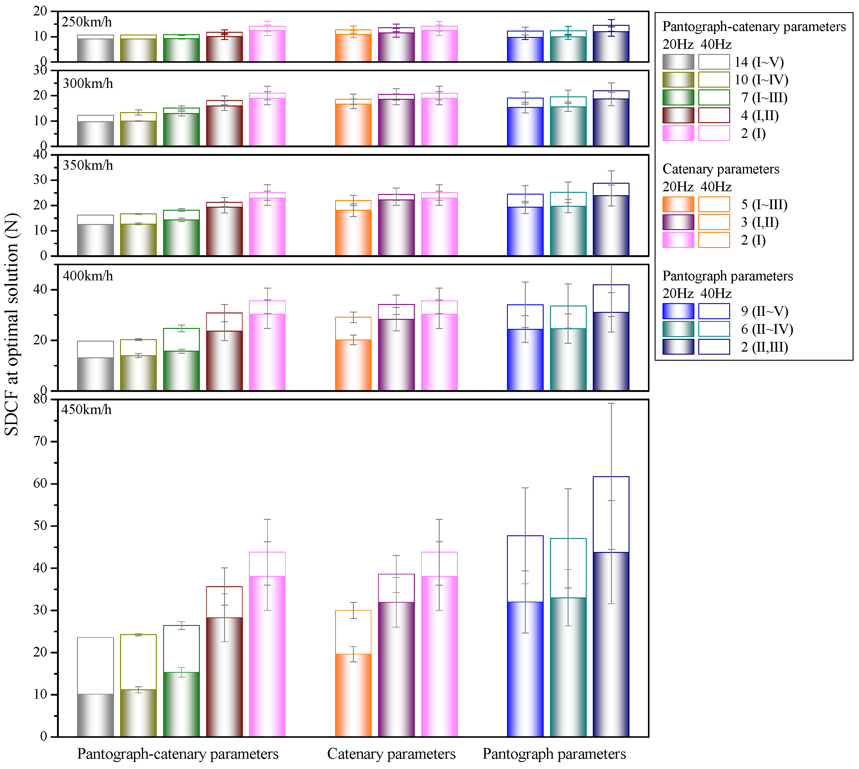Figure 8 provides the mean and standard deviation of SDCF at the optimal solutions for 100 samples in each operating condition.

Compared to the optimization effects of jointly optimizing all 14 pantograph–catenary parameters at 250 km/h, the optimization results for 5 catenary parameters, or 6 pantograph parameters at Classes II-IV, or 4 pantograph–catenary parameters at Classes I-II, as well as combinations of these parameters, show similar performance. At 300 km/h and above, the optimization effects for 11 pantograph–catenary parameters, excluding (c₃, c₂, k₁), are comparable. However, the optimization performance of other parameter combinations is notably inadequate, and the performance gap widens as the operating speed increases or the number of decision variables decreases.

To further elaborate, in comparison to optimizing the five catenary parameters at speeds of 300 km/h and below, optimizing the two Class I catenary parameters (T_c, A_c) yields similar effects. As the speed increases, it becomes necessary to consider simultaneously optimizing the three catenary parameters for Classes II-III. In comparison to optimizing the nine pantograph parameters across all speed ranges, optimizing the six pantograph parameters (m₃, c₁, m₁, m₂, k₃, k₂) at Classes II-IV produces similar results, and the Class V parameters (c₃, c₂, k₁) can be ignored.

In summary, at medium speeds, it is sufficient to conduct optimization designs with a smaller number of pantograph–catenary parameters, such as individually optimizing the five catenary parameters (T_c, A_c, A_m, L, T_m), individually optimizing the six pantograph parameters (m₃, c₁, m₁, m₂, k₃, k₂), or jointly optimizing the four pantograph–catenary parameters (m₃, T_c, A_c, A_m). However, at high and superhigh speeds, it is advisable to choose the optimization scheme with the highest cost-effectiveness based on the feasibility of the engineering project, as indicated in Figure 8.

5. Conclusions and Future Work

Based on Latin Hypercube Sampling and a validated finite element model of the pantograph–catenary, a database for the pantograph–catenary interaction examples was established. Using a feedforward neural network, a surrogate model for the SDCF with respect to operating speed and 14 pantograph–catenary parameters was constructed. This surrogate model exhibits strong generalization ability and can accurately predict the SDCF for unknown samples.

With the surrogate model and the variance-based method, the first-order and total sensitivities of the SDCF to the pantograph–catenary parameters were calculated across the entire speed range and different frequency bands. Utilizing the k-means clustering algorithm, the pantograph–catenary parameters were categorized into Classes I to V. Among the pantograph–catenary parameters, T_c and A_c fall into Class I, as their impact on the SDCF is significantly higher than that of the other pantograph–catenary parameters, while k₁, c₃, and c₂ fall into Class V, the influence of which can be neglected. Additionally, at speeds of 400 km/h and above, the coupling effects between catenary parameters need to be considered, and at speeds of 450 km/h, the influence of low-pass filtering frequency on the sensitivity of pantograph–catenary parameters also needs to be considered.

Following a stepwise reduction in sensitivity class, 10 sets of decision vectors consisting of pantograph–catenary parameters, catenary parameters, and pantograph parameters were obtained. Using the surrogate model and the SCSA, optimization was performed across the entire speed range with the objective of minimizing the SDCF. At a medium speed of 250 km/h, it is sufficient to optimize the pantograph–catenary, catenary, or pantograph parameters at higher sensitivity classes to achieve the desired optimization results. However, at higher speeds and above, the number of optimized parameters needs to be increased. Furthermore, k₁, c₃, and c₂ can be neglected under all operating conditions.

In the future, a pantograph–catenary model that can more accurately predict its real dynamic performance is required to be obtained, such as a pantograph model that considers more degrees of freedom, medium–high frequency, and other low-frequency vibrations, and a three-dimensional catenary model that considers stagger.

References

- Bruni, S.; Bucca, G.; Carnevale, M.; Collina, A.; Facchinetti, A. Pantograph-catenary interaction: Recent achievements and future research challenges. Int. J. Rail Transp. 2017, 6, 57–82. [Google Scholar] [CrossRef]
- Zhang, W.H.; Zou, D.; Tan, M.Y.; Zhou, N.; Li, R.P.; Mei, G.M. Review of pantograph and catenary interaction. Front. Mech. Eng. 2018, 13, 311–322. [Google Scholar] [CrossRef]
- Wu, G.N.; Dong, K.L.; Xu, Z.L.; Xiao, S.; Wei, W.F.; Chen, H.; Li, J.; Huang, Z.L.; Li, J.W.; Gao, G.Q.; et al. Pantograph–catenary electrical contact system of high-speed railways: Recent progress, challenges, and outlooks. Railw. Eng. Sci. 2022, 30, 437–467. [Google Scholar] [CrossRef]
- EN50317:2012; Railway Applications–Current Collection Systems-Requirements for and Validation of Measurements of the Dynamic Interaction between Pantograph and Overhead Contact Line. European Parliament: Strasbourg, France, 2012.
- EN50318:2018; Railway Applications–Current Collection Systems-Validation of Simulation of the Dynamic Interaction between Pantograph and Overhead Contact Line. European Parliament: Strasbourg, France, 2018.
- EN50367:2020; Railway Applications—Criteria to Achieve Technical Compatibility between Pantographs and Overhead Contact Line. European Parliament: Strasbourg, France, 2020.
- Park, T.J.; Han, C.S.; Jang, J.H. Dynamic sensitivity analysis for the pantograph of a high-speed rail vehicle. J. Sound Vib. 2003, 266, 235–260. [Google Scholar] [CrossRef]
- Wu, M.Z.; Liu, Y.; Xu, X.H. Sensitivity analysis and optimization on parameters of high speed pantograph-catenary system. Chin. J. Theor. Appl. Mech. 2021, 53, 75–83. [Google Scholar]
- Chen, K.; Song, Y.; Lu, X.B.; Duan, F.C. Sensitivity Analysis and Optimisation of Key Parameters for Railway Rigid Overhead System and Pantograph. Sustainability 2023, 15, 15. [Google Scholar] [CrossRef]
- Zhang, J.; Liu, W.Z.; Zhang, Z.F. Sensitivity analysis and research on optimisation methods of design parameters of high-speed railway catenary. IET Electr. Syst. Transp. 2019, 9, 150–156. [Google Scholar] [CrossRef]
- Pombo, J.; Ambrósio, J. Influence of pantograph suspension characteristics on the contact quality with the catenary for high speed trains. Comput. Struct. 2012, 110, 32–42. [Google Scholar] [CrossRef]
- Kim, J.W.; Yu, S.N. Design variable optimization for pantograph system of high-speed train using robust design technique. Int. J. Precis. Eng. Manuf. 2013, 14, 267–273. [Google Scholar] [CrossRef]
- Ambrósio, J.; Pombo, J.; Pereira, M. Optimization of high-speed railway pantographs for improving pantograph-catenary contact. Theor. Appl. Mech. Lett. 2013, 3, 013006. [Google Scholar] [CrossRef]
- Wang, H.L.; Zheng, D.Y.; Huang, P.; Yan, W.Y. Design optimisation of railway pantograph-catenary systems with multiple objectives. Veh. Syst. Dyn. 2023, 61, 2953–2975. [Google Scholar] [CrossRef]
- Huang, G.Z.; Wu, G.N.; Yang, Z.F.; Chen, X.; Wei, W.F. Development of surrogate models for evaluating energy transfer quality of high-speed railway pantograph-catenary system using physics-based model and machine learning. Appl. Energy 2023, 333, 12. [Google Scholar] [CrossRef]
- Lee, J.H.; Kim, Y.G.; Paik, J.S.; Park, T.W. Performance evaluation and design optimization using differential evolutionary algorithm of the pantograph for the high-speed train. J. Mech. Sci. Technol. 2012, 26, 3253–3260. [Google Scholar] [CrossRef]
- Wang, X.Y.; Nian, X.H.; Chu, X.Y.; Yue, P.C. Research on dynamic performance and parameter optimization of the high-speed pantograph and catenary system. In Proceedings of the 2017 Prognostics and System Health Management Conference (Phm-Harbin), Harbin, China, 9–12 July 2017. [Google Scholar]
- Su, K.X.; Zhang, J.W.; Zhang, J.W.; Yan, T.; Mei, G.M. Optimisation of current collection quality of high-speed pantograph-catenary system using the combination of artificial neural network and genetic algorithm. Veh. Syst. Dyn. 2022, 61, 260–285. [Google Scholar] [CrossRef]
- Zhou, R.; Xu, X.H. Dynamic parameter optimization of high-speed pantograph base on swarm intelligence and machine learning. Int. J. Appl. Mech. 2023, 15, 19. [Google Scholar] [CrossRef]
- McKay, M.D.; Beckman, R.J.; Conover, W.J. A comparison of three methods for selecting values of input variables in the analysis of output from a computer code. Technometrics 1979, 21, 239–245. [Google Scholar]
- Wu, M.Z.; Xu, X.H.; Yan, Y.Z.; Luo, Y.; Huang, S.J.; Wang, J.S. Multi-parameter joint optimization for double-strip high-speed pantographs to improve pantograph-catenary interaction quality. Acta Mech. Sin. 2022, 38, 11. [Google Scholar] [CrossRef]
- Zhou, Z.H. Machine Learning, 1st ed.; Tsinghua University Press: Beijing, China, 2016; pp. 105–106. [Google Scholar]
- Qin, Y.; Zhang, Y.; Cheng, X.Q.; Jia, L.M.; Xing, Z.Y. An analysis method for correlation between catenary irregularities and pantograph-catenary contact force. J. Cent. South Univ. 2014, 21, 3353–3360. [Google Scholar] [CrossRef]
- Saltelli, A.; Tarantola, S.; Campolongo, F.; Ratto, M. Sensitivity Analysis in Practice: A Guide to Assessing Scientific Models. J. R. Stat. Soc. Ser. A Stat. Soc. 2004, 168, 466. [Google Scholar]
- Tian, W. A review of sensitivity analysis methods in building energy analysis. Renew. Sustain. Energy Rev. 2013, 20, 411–419. [Google Scholar] [CrossRef]
- Sobol, I. On sensitivity estimation for nonlinear mathematical models. Mat. Model. 1990, 2, 112–118. [Google Scholar]
- Yang, J. Convergence and uncertainty analyses in Monte-Carlo based sensitivity analysis. Environ. Model. Softw. 2011, 26, 444–457. [Google Scholar] [CrossRef]
- Saltelli, A. Making best use of model evaluations to compute sensitivity indices. Comput. Phys. Commun. 2002, 145, 280–297. [Google Scholar] [CrossRef]
- Iwanaga, T.; Usher, W.; Herman, J. Toward SALib 2.0: Advancing the accessibility and interpretability of global sensitivity analyses. Socio-Environ. Syst. Model. 2022, 4, 18155. [Google Scholar] [CrossRef]
- Herman, J.; Usher, W. SALib: An open-source Python library for sensitivity analysis. J. Open Source Softw. 2017, 2, 1–2. [Google Scholar] [CrossRef]