
Modeling the Spatial Distribution of Population Based on Random Forest and Parameter Optimization Methods: A Case Study of Sichuan, China

Abstract
1. Introduction
2. Study Area and Data
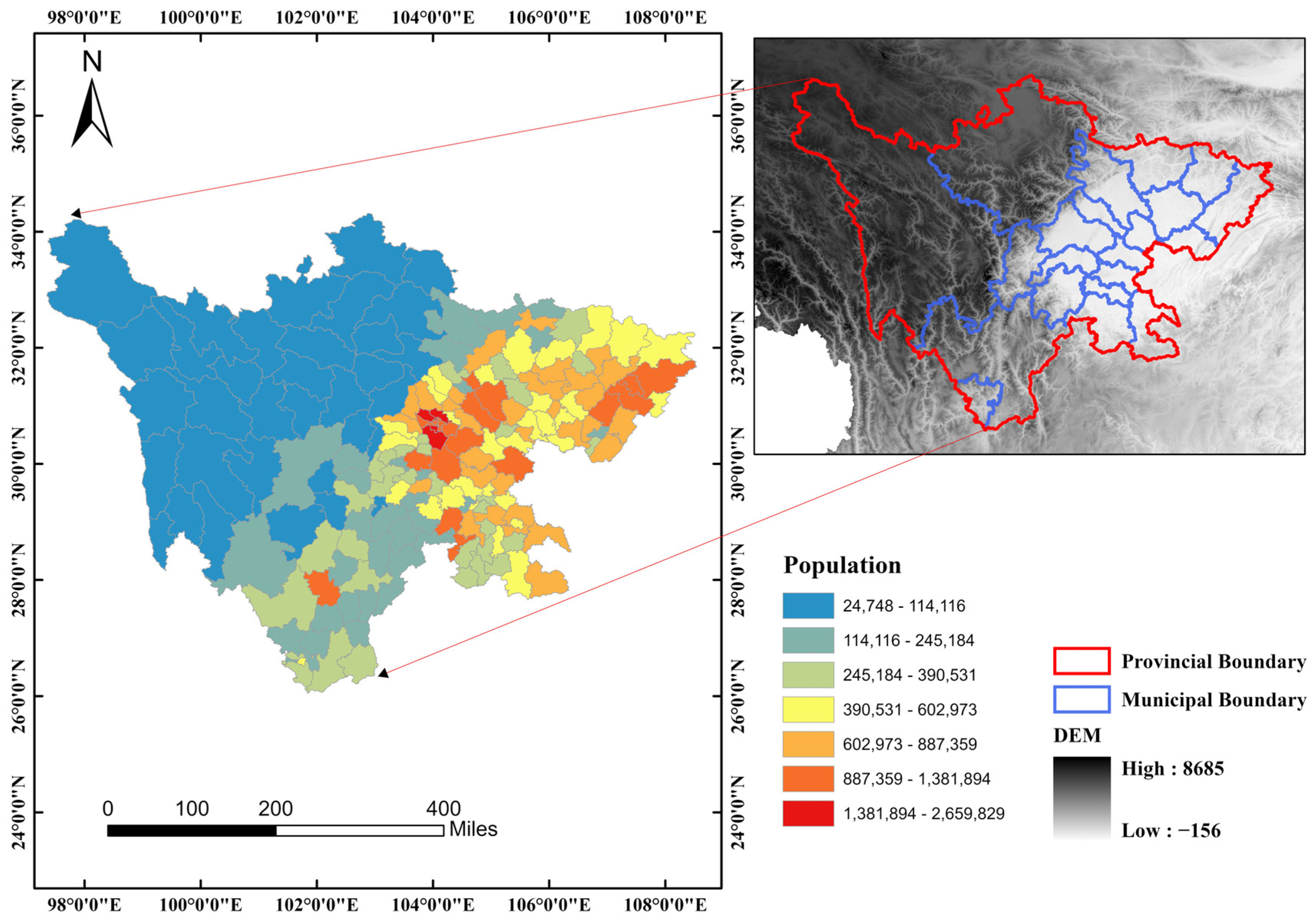
2.1. Study Area
2.2. Data Preparation
3. Methods
3.1. Data Processing
3.1.1. Geographical Information Data Processing
3.1.2. Nighttime Light Data Processing
- 1.
- Radiometric Correction
- 2.
- Background Noise and Abnormal Value Correction
- 3.
- Stable Light Source Extraction
3.1.3. POI Data Processing
3.2. Feature Selection
3.2.1. Pearson Correlation Coefficient Method
3.2.2. Variance Threshold Method
3.2.3. ReliefF Method
3.2.4. Recursive Feature Elimination Method
3.3. Random Forest Model Construction and Parameters Optimization
3.3.1. Model Construction
3.3.2. Model Parameter Optimization
- (a)
- Data Splitting: We partition the training dataset into 5 independent and equally sized subsets, referred to as “folds,” and no replacement is made.
- (b)
- Model Training and Validation: In each training round, we perform 5 iterations, where in each iteration, 4 of the folds are chosen, and we combine them with parameter optimization methods to train the model. The remaining 1 fold is used as the validation set, and we calculate the R2_score to evaluate the model produced during this training session. After 5 iterations, we obtain 5 performance evaluation metrics.
- (c)
- Model Evaluation: We compute the average of the performance metrics from all 5 iterations and use it as the performance metric for that round of model training.
3.4. Population Spatialization
4. Results
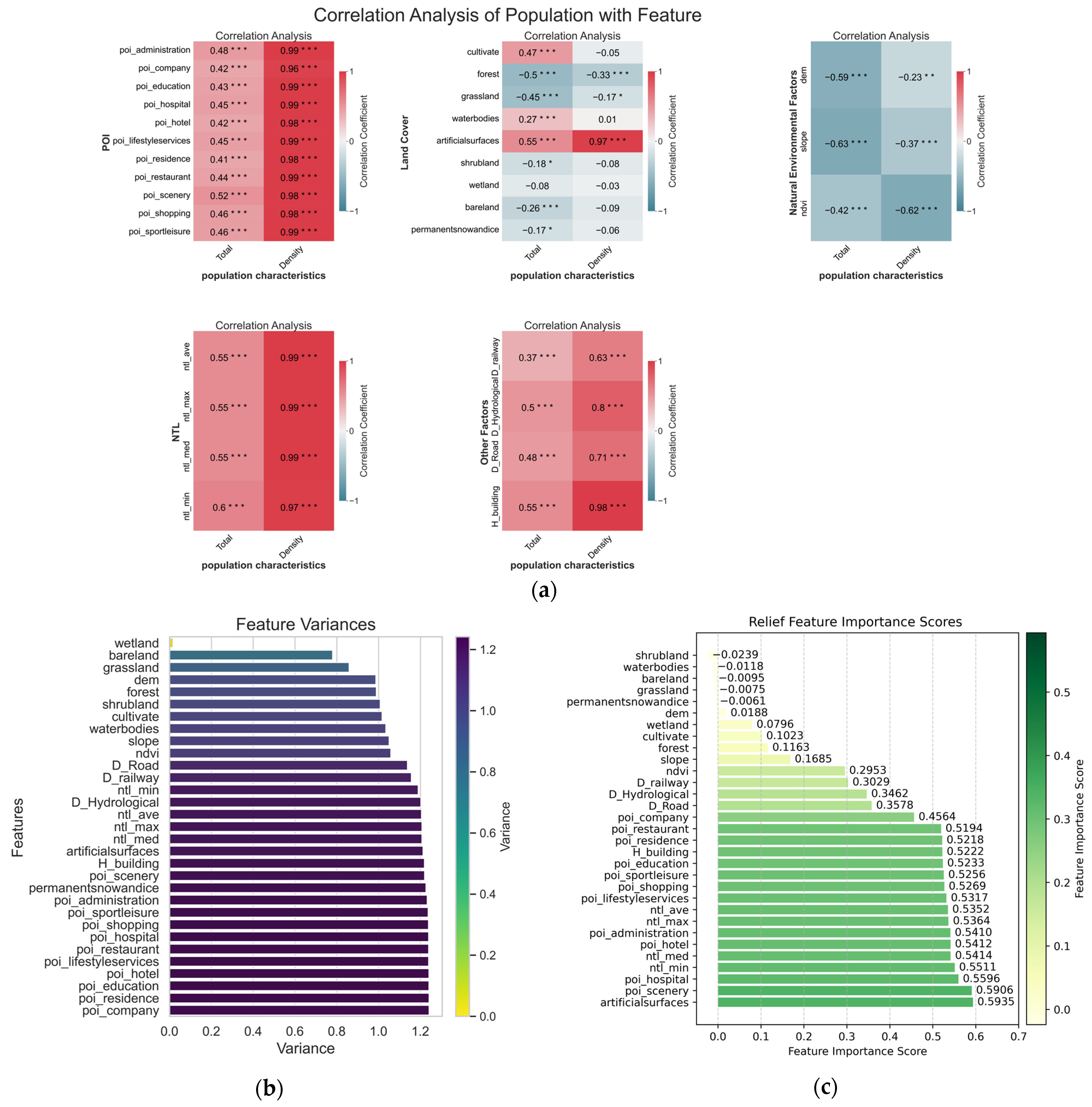
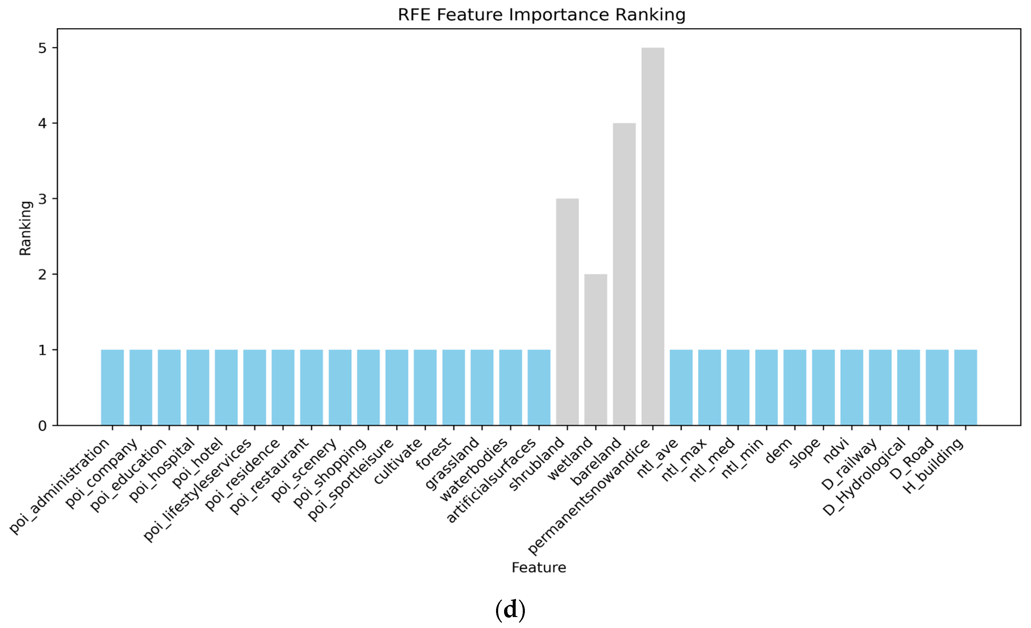
4.1. Feature Selection Results
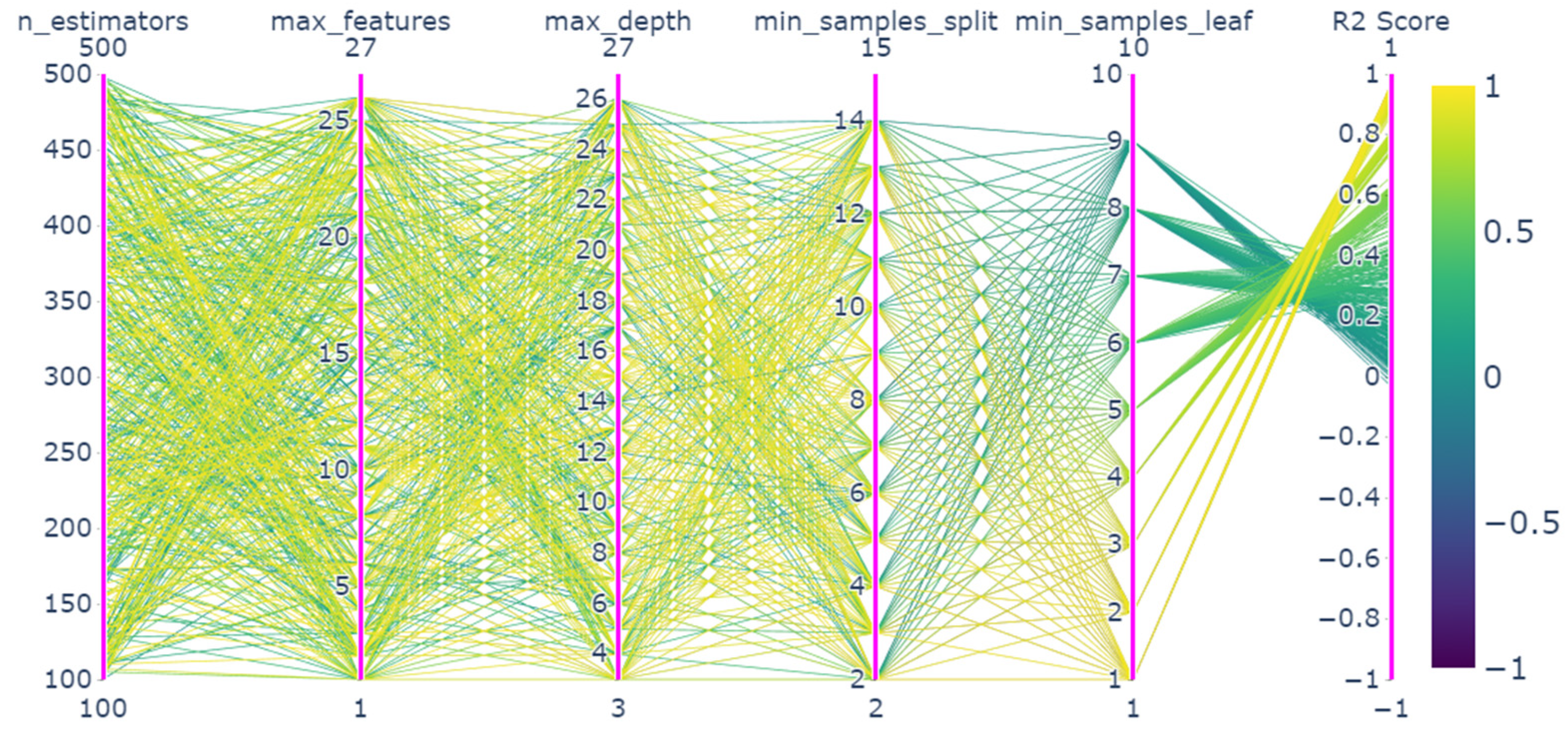
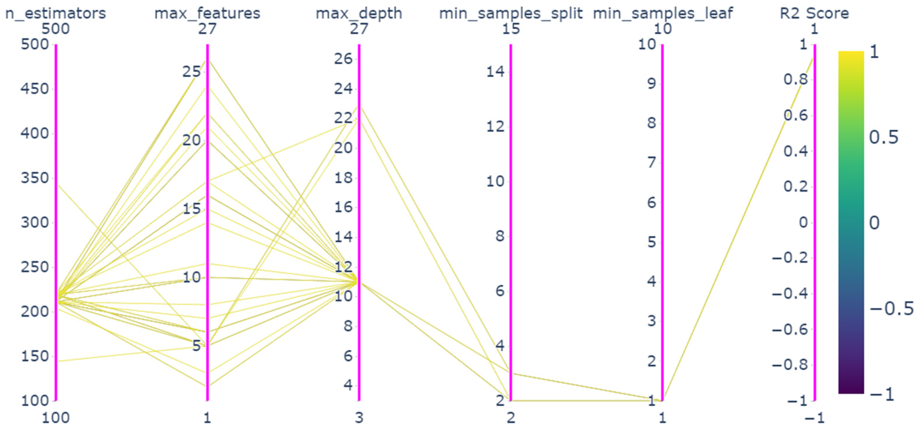
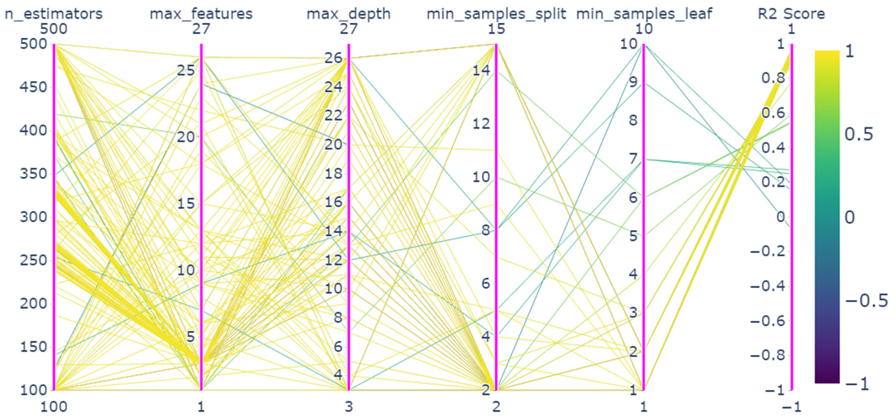
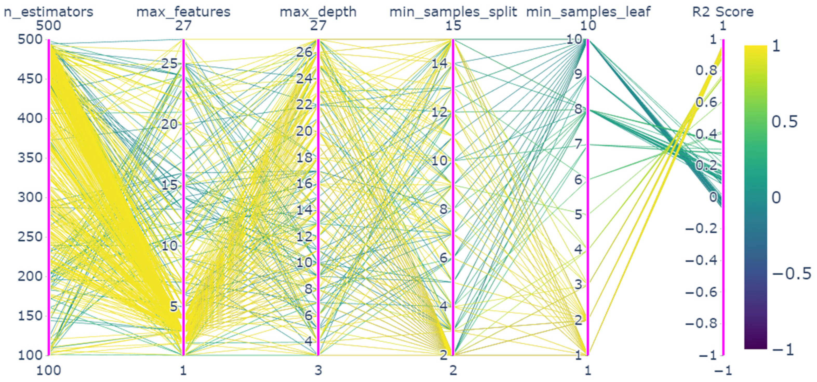
4.2. Parameter Optimization Results
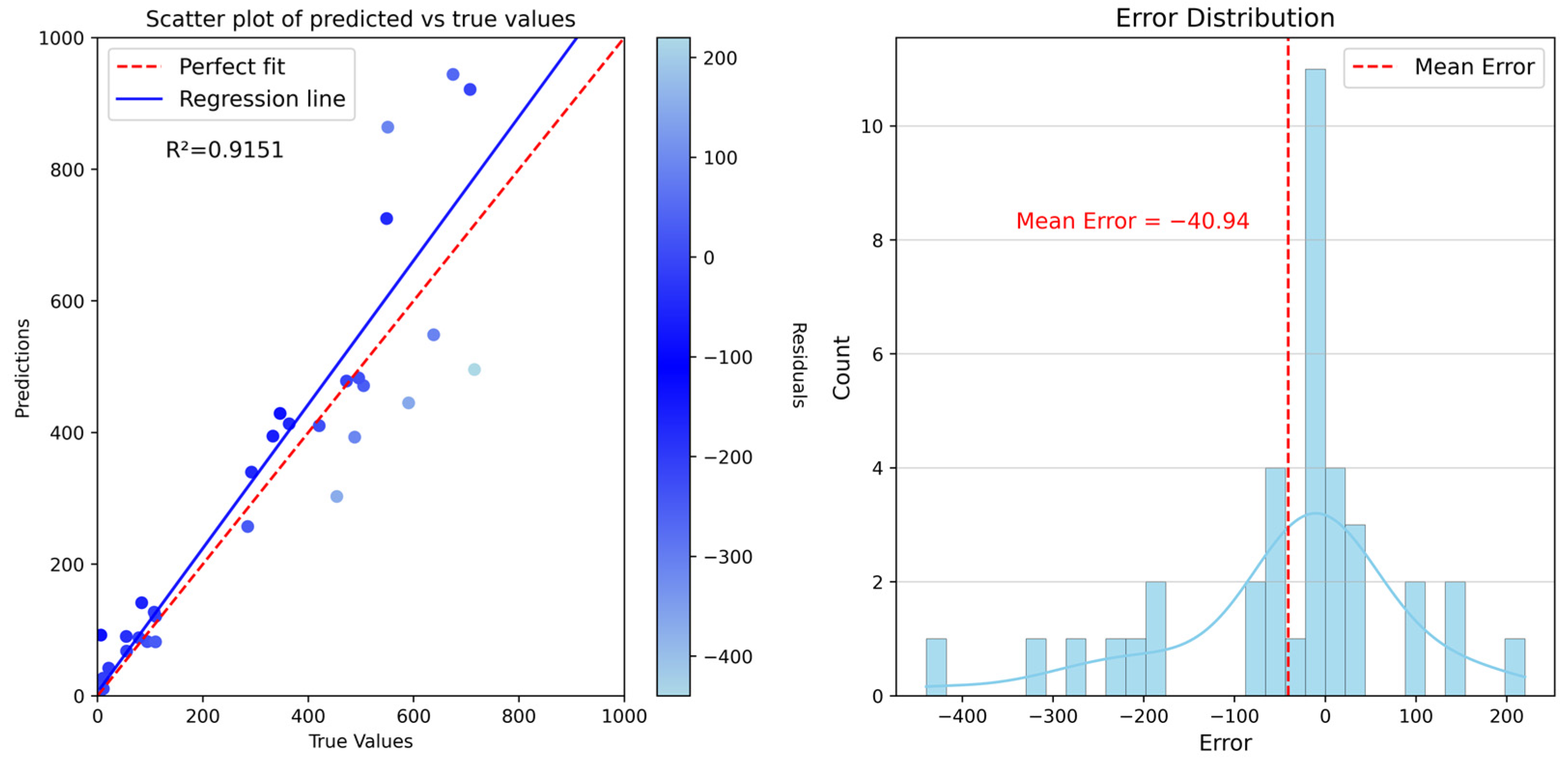
4.3. Model Accuracy Validation
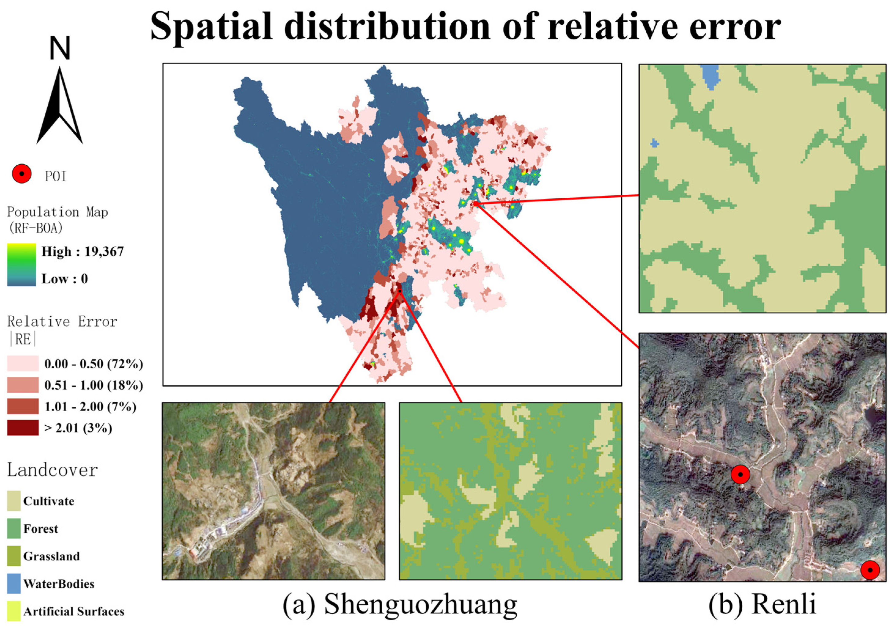
4.4. Population Spatialization Result Validation and Error Analysis
5. Discussion
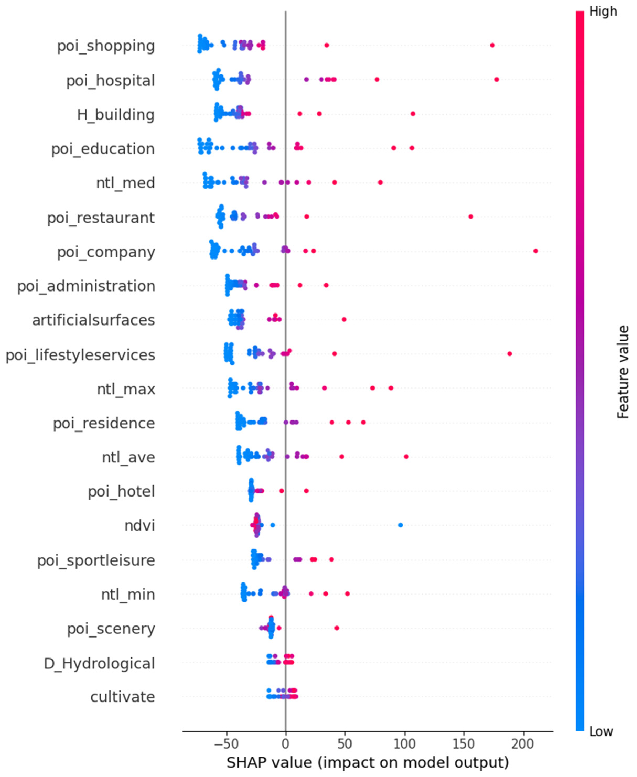
5.1. Feature Importance Analysis
5.2. Comparison with Other Datasets
6. Conclusions
Author Contributions
Funding
Institutional Review Board Statement
Informed Consent Statement
Data Availability Statement
Conflicts of Interest
References
- Bird, J.; Lebrand, M.; Venables, A.J. The belt and road initiative: Reshaping economic geography in Central Asia? J. Dev. Econ. 2020, 144, 102441. [Google Scholar] [CrossRef]
- Andrade-Pacheco, R.; Savory, D.J.; Midekisa, A. Household electricity access in Africa (2000–2013): Closing information gaps with model-based geostatistics. PLoS ONE 2019, 14, e0214635. [Google Scholar] [CrossRef]
- Tusting, L.S.; Bisanzio, D.; Alabaster, G.; Cameron, E.; Cibulskis, R.; Davies, M.; Flaxman, S.; Gibson, H.; Knudsen, J.; Mbogo, C.; et al. Mapping changes in housing in sub-Saharan Africa from 2000 to 2015. Nature 2019, 568, 391–394. [Google Scholar] [CrossRef] [PubMed]
- Eales, A.; Alsop, A.; Frame, D.; Strachan, S.; Galloway, S. Assessing the market for solar photovoltaic (PV) microgrids in Malawi. Hapres J. Sustain. Res. 2020, 2, e200008. [Google Scholar]
- Melchiorri, M.; Pesaresi, M.; Florczyk, A.J.; Corbane, C.; Kemper, T. Principles and applications of the global human settlement layer as baseline for the land use efficiency indicator—SDG 11.3. 1. ISPRS Int. J. Geoinf. 2019, 8, 96. [Google Scholar] [CrossRef]
- Ehrlich, D.; Melchiorri, M.; Florczyk, A.J.; Pesaresi, M.; Kemper, T.; Corbane, C.; Corbane, C.; Freire, S.; Schiavina, M.; Siragusa, A. Remote sensing derived built-up area and population density to quantify global exposure to five natural hazards over time. Remote Sens. 2018, 10, 1378. [Google Scholar] [CrossRef]
- Dasgupta, S.; Laplante, B.; Murray, S.; Wheeler, D. Exposure of developing countries to sea-level rise and storm surges. Clim. Chang. 2011, 106, 567–579. [Google Scholar] [CrossRef]
- Aubrecht, C.; Özceylan, D.; Steinnocher, K.; Freire, S. Multi-level geospatial modeling of human exposure patterns and vulnerability indicators. Nat. Hazards 2013, 68, 147–163. [Google Scholar] [CrossRef]
- Azar, D.; Engstrom, R.; Graesser, J.; Comenetz, J. Generation of fine-scale population layers using multi-resolution satellite imagery and geospatial data. Remote Sens. Environ. 2013, 130, 219–232. [Google Scholar] [CrossRef]
- Lai, S.; Bogoch, I.I.; Ruktanonchai, N.W.; Watts, A.; Lu, X.; Yang, W.; Yu, H.; Khan, K.; Tatem, A.J. Assessing spread risk of COVID-19 within and beyond China in early 2020. Data Sci. Manag. 2022, 5, 212–218. [Google Scholar] [CrossRef]
- Thomson, D.R.; Linard, C.; Vanhuysse, S.; Steele, J.E.; Shimoni, M.; Siri, J.; José Siri, M.; Caiaffa, W.T.; Rosenberg, M.; Wolff, E.; et al. Extending data for urban health decision-making: A menu of new and potential neighborhood-level health determinants datasets in LMICs. J. Urban. Health 2019, 96, 514–536. [Google Scholar] [CrossRef] [PubMed]
- James, W.H.; Tejedor-Garavito, N.; Hanspal, S.E.; Campbell-Sutton, A.; Hornby, G.M.; Pezzulo, C.; Nilsen, K.; Sorichetta, A.; Ruktanonchai, C.W.; Carioli, A.; et al. Gridded birth and pregnancy datasets for Africa, Latin America and the Caribbean. Sci. Data 2018, 5, 180090. [Google Scholar] [CrossRef] [PubMed]
- Cai, Q.; Rushton, G.; Bhaduri, B.; Bright, E.; Coleman, P. Estimating small-area populations by age and sex using spatial interpolation and statistical inference methods. Trans. GIS 2006, 10, 577–598. [Google Scholar] [CrossRef]
- Goodchild, M.F.; Anselin, L.; Deichmann, U. A framework for the areal interpolation of socioeconomic data. Environ. Plan. A 1993, 25, 383–397. [Google Scholar] [CrossRef]
- Xie, Z. A framework for interpolating the population surface at the residential-housing-unit level. GIsci Remote Sens. 2006, 43, 233–251. [Google Scholar] [CrossRef]
- Jin, Y.; Liu, R.; Fan, H.; Li, P.; Liu, Y.; Jia, Y. Multi-Resolution Population Mapping Based on a Stepwise Downscaling Approach Using Multisource Data. Remote Sens. 2023, 15, 1947. [Google Scholar] [CrossRef]
- Guo, H.; Zhu, W. A review on the spatial disaggregation of socioeconomic statistical data. Acta Geogr. Sin. 2022, 77, 2650–2667. [Google Scholar]
- Zeng, C.; Zhou, Y.; Wang, S.; Yan, F.; Zhao, Q. Population spatialization in China based on night-time imagery and land use data. Int. J. Remote Sens. 2011, 32, 9599–9620. [Google Scholar] [CrossRef]
- Lo, C.P. Population estimation using geographically weighted regression. GIsci Remote Sens. 2008, 45, 131–148. [Google Scholar] [CrossRef]
- Huang, Y.; Zhao, C.; Song, X.; Chen, J.; Li, Z. A semi-parametric geographically weighted (S-GWR) approach for modeling spatial distribution of population. Ecol. Indic. 2018, 85, 1022–1029. [Google Scholar] [CrossRef]
- Chi, G.; Zhu, J. Spatial regression models for demographic analysis. Popul. Res. Policy Rev. 2008, 27, 17–42. [Google Scholar] [CrossRef]
- Liu, X.H.; Kyriakidis, P.C.; Goodchild, M.F. Population-density estimation using regression and area-to-point residual kriging. Int. J. Geogr. Inf. Sci. 2008, 22, 431–447. [Google Scholar] [CrossRef]
- Friedman, J.H. Greedy function approximation: A gradient boosting machine. Ann. Stat. 2001, 29, 1189–1232. [Google Scholar] [CrossRef]
- Folberth, C.; Baklanov, A.; Balkovič, J.; Skalský, R.; Khabarov, N.; Obersteiner, M. Spatio-temporal downscaling of gridded crop model yield estimates based on machine learning. Agric. For. Meteorol. 2019, 264, 1–15. [Google Scholar] [CrossRef]
- Zhao, X.; Xia, N.; Xu, Y.; Huang, X.; Li, M. Mapping population distribution based on XGBoost using multisource data. IEEE J. Sel. Top. Appl. Earth Obs. Remote Sens. 2021, 14, 11567–11580. [Google Scholar] [CrossRef]
- Breiman, L. Bagging predictors. Mach. Learn. 1996, 24, 123–140. [Google Scholar] [CrossRef]
- Qiu, G.; Bao, Y.; Yang, X.; Wang, C.; Ye, T.; Stein, A.; Jia, P. Local population mapping using a random forest model based on remote and social sensing data: A case study in Zhengzhou, China. Remote Sens. 2020, 12, 1618. [Google Scholar] [CrossRef]
- Stevens, F.R.; Gaughan, A.E.; Linard, C.; Tatem, A.J. Disaggregating census data for population mapping using random forests with remotely-sensed and ancillary data. PLoS ONE 2015, 10, e0107042. [Google Scholar] [CrossRef]
- Li, K.; Chen, Y.; Li, Y. The random forest-based method of fine-resolution population spatialization by using the international space station nighttime photography and social sensing data. Remote Sens. 2018, 10, 1650. [Google Scholar] [CrossRef]
- Ye, T.; Zhao, N.; Yang, X.; Ouyang, Z.; Liu, X.; Chen, Q.; Hu, K.; Yue, W.; Qi, J.; Li, Z.; et al. Improved population mapping for China using remotely sensed and points-of-interest data within a random forests model. Sci. Total Environ. 2019, 658, 936–946. [Google Scholar] [CrossRef]
- Liu, L.; Cheng, G.; Yang, J.; Cheng, Y. Population Spatialization in Zhengzhou City Based on Multi-source Data and Random Forest Model. Front. Earth Sci. 2023, 11, 1092664. [Google Scholar] [CrossRef]
- He, M.; Xu, Y.; Li, N. Population spatialization in Beijing city based on machine learning and multisource remote sensing data. Remote Sens. 2020, 12, 1910. [Google Scholar] [CrossRef]
- Doupe, P.; Bruzelius, E.; Faghmous, J.; Ruchman, S.G. Equitable development through deep learning: The case of sub-national population density estimation. In Proceedings of the 7th Annual Symposium on Computing for Development, Nairobi, Kenya, 18–20 November 2016; pp. 1–10. [Google Scholar]
- Xing, X.; Huang, Z.; Cheng, X.; Zhu, D.; Kang, C.; Zhang, F.; Liu, Y. Mapping human activity volumes through remote sensing imagery. IEEE J. Sel. Top. Appl. Earth Obs. Remote Sens. 2020, 13, 5652–5668. [Google Scholar] [CrossRef]
- Tobler, W.; Deichmann, U.; Gottsegen, J.; Maloy, K. World population in a grid of spherical quadrilaterals. Int. J. Popul. Geogr. 1997, 3, 203–225. [Google Scholar] [CrossRef]
- Da Costa, J.N.; Bielecka, E.; Calka, B. Uncertainty quantification of the global rural-urban mapping project over Polish census data. In Environmental Engineering, Proceedings of the International Conference on Environmental Engineering, Vilnius, Lithuania, 27–28 April 2017; ICEE, Vilnius Gediminas Technical University, Department of Construction Economics & Property: Vilnius, Lithuania; Volume 10, pp. 1–7.
- Dobson, J.E.; Bright, E.A.; Coleman, P.R.; Durfee, R.C.; Worley, B.A. LandScan: A global population database for estimating populations at risk. Photogramm. Eng. Remote Sens. 2000, 66, 849–857. [Google Scholar]
- Tatem, A.J. WorldPop, open data for spatial demography. Sci. Data 2017, 4, 170004. [Google Scholar] [CrossRef] [PubMed]
- Zhou, Y.; Ma, M.; Shi, K.; Peng, Z. Estimating and interpreting fine-scale gridded population using random forest regression and multisource data. ISPRS Int. J. Geoinf. 2020, 9, 369. [Google Scholar] [CrossRef]
- Gunasekera, R.; Ishizawa, O.; Aubrecht, C.; Blankespoor, B.; Murray, S.; Pomonis, A.; Daniell, J. Developing an adaptive global exposure model to support the generation of country disaster risk profiles. Earth Sci. Rev. 2015, 150, 594–608. [Google Scholar] [CrossRef]
- Sabesan, A.; Abercrombie, K.; Ganguly, A.R.; Bhaduri, B.; Bright, E.A.; Coleman, P.R. Metrics for the comparative analysis of geospatial datasets with applications to high-resolution grid-based population data. GeoJournal 2007, 69, 81–91. [Google Scholar] [CrossRef]
- Bai, Z.; Wang, J.; Wang, M.; Gao, M.; Sun, J. Accuracy assessment of multi-source gridded population distribution datasets in China. Sustainability 2018, 10, 1363. [Google Scholar] [CrossRef]
- Zhang, J.; Zhu, W.; Zhu, L.; Cui, Y.; He, S.; Ren, H. Topographical relief characteristics and its impact on population and economy: A case study of the mountainous area in western Henan, China. J. Geogr. Sci. 2019, 29, 598–612. [Google Scholar] [CrossRef]
- Lu, D.; Tian, H.; Zhou, G.; Ge, H. Regional mapping of human settlements in southeastern China with multisensor remotely sensed data. Remote Sens. Environ. 2008, 112, 3668–3679. [Google Scholar] [CrossRef]
- Amaral, S.; Câmara, G.; Monteiro, A.M.V.; Quintanilha, J.A.; Elvidge, C.D. Estimating population and energy consumption in Brazilian Amazonia using DMSP night-time satellite data. Comput. Environ. Urban. Syst. 2005, 29, 179–195. [Google Scholar] [CrossRef]
- Bakillah, M.; Liang, S.; Mobasheri, A.; Jokar Arsanjani, J.; Zipf, A. Fine-resolution population mapping using OpenStreetMap points-of-interest. Int. J. Geogr. Inf. Sci. 2014, 28, 1940–1963. [Google Scholar] [CrossRef]
- Wang, M.; Wang, Y.; Li, B.; Cai, Z.; Kang, M. A population spatialization model at the building scale using random forest. Remote Sens. 2022, 14, 1811. [Google Scholar] [CrossRef]
- Wu, W.B.; Ma, J.; Banzhaf, E.; Meadows, M.E.; Yu, Z.W.; Guo, F.X.; Sengupta, D.; Cai, X.; Zhao, B. A first Chinese building height estimate at 10 m resolution (CNBH-10 m) using multi-source earth observations and machine learning. Remote Sens. Environ. 2023, 291, 113578. [Google Scholar] [CrossRef]
- Holben, B.N. Characteristics of maximum-value composite images from temporal AVHRR data. Int. J. Remote Sens. 1986, 7, 1417–1434. [Google Scholar] [CrossRef]
- Li, X.; Xu, H.; Chen, X.; Li, C. Potential of NPP-VIIRS nighttime light imagery for modeling the regional economy of China. Remote Sens. 2013, 5, 3057–3081. [Google Scholar] [CrossRef]
- Biswas, N.; Ali, M.M.; Rahaman, M.A.; Islam, M.; Mia, M.R.; Azam, S.; Ahmed, k.; e Moni, M.A. Machine Learning-Based Model to Predict Heart Disease in Early Stage Employing Different Feature Selection Techniques. Biomed. Res. Int. 2023, 2023, 6864343. [Google Scholar] [CrossRef]
- Mao, Z.; Han, H.; Zhang, H.; Ai, B. Population spatialization at building scale based on residential population index—A case study of Qingdao city. PLoS ONE 2022, 17, e0269100. [Google Scholar] [CrossRef]
- Lu, P.; Ye, L.; Pei, M.; Zhao, Y.; Dai, B.; Li, Z. Short-term wind power forecasting based on meteorological feature extraction and optimization strategy. Renew. Energy 2022, 184, 642–661. [Google Scholar] [CrossRef]
- Robnik-Šikonja, M.; Kononenko, I. Theoretical and empirical analysis of ReliefF and RReliefF. Mach. Learn. 2003, 53, 23–69. [Google Scholar] [CrossRef]
- Subbiah, S.S.; Chinnappan, J. Deep learning based short term load forecasting with hybrid feature selection. Electric Pow. Syst. Res. 2022, 210, 108065. [Google Scholar] [CrossRef]
- Wakjira, T.G.; Ibrahim, M.; Ebead, U.; Alam, M.S. Explainable machine learning model and reliability analysis for flexural capacity prediction of RC beams strengthened in flexure with FRCM. Eng. Struct. 2022, 255, 113903. [Google Scholar] [CrossRef]
- Lundberg, S.M.; Lee, S.I. A unified approach to interpreting model predictions. NeurIPS 2017, 30, 4768–4777. [Google Scholar]
- Meng, Y.; Yang, N.; Qian, Z.; Zhang, G. What makes an online review more helpful: An interpretation framework using XGBoost and SHAP values. J. Theor. Appl. Electron. Commer. Res. 2020, 16, 466–490. [Google Scholar] [CrossRef]


| Category | Name | Time | Spatial Scale | Format | Source |
|---|---|---|---|---|---|
| (a) Demographic data | Census data | 2020 | county-level and township-level | Table (csv) | http://www.citypopulation.de/ (accessed on 21 February 2022) |
| (b) Basic geographic information data | Administrative boundaries data | 2020 | 1:100 w | Vector (Polygon) | https://www.webmap.cn/ (accessed on 19 October 2022) |
| Road network | 2021 Version | 1:100 w | Vector (Polyline) | https://www.webmap.cn/ (accessed on 19 October 2022) | |
| River network | 2021 Version | 1:100 w | Vector (Polyline) | https://www.webmap.cn/ (accessed on 19 October 2022) | |
| (c) Natural environmental data | ASTER GDEM v3 | 2000 | 30 m | Raster | https://www.gscloud.cn/ (accessed on 23 October 2022) |
| Globeland 30 | 2020 | 30 m | Raster | http://www.globallandcover.com/ (accessed on 7 April 2022) | |
| NDVI (Landsat 8) | 2020 | 100 m | Raster | https://www.usgs.gov/ (accessed on 20 October 2022) | |
| (d) Building height data | CNBH-10m | 2020 | 10 m | Raster | https://zenodo.org/ (accessed on 6 June 2023) |
| (e) Nighttime light (NTL) data | NPP-VIIRS v2.1 | 2020 | 500 m | Raster | https://eogdata.mines.edu/ (accessed on 23 October 2022) |
| LJ-01 | 2019 | 130 m | Raster | http://datasearch.hbeos.org.cn:3000/ (accessed on 25 October 2022) | |
| (f) Social perception data | Point of interest (POI) | —— | —— | Vector (Point) | https://ditu.amap.com/ (accessed on 9 March 2022) |
| NO. | Reclassified Label | Examples | Quantity |
|---|---|---|---|
| 1 | poi_administration | Authority, federation, committee, fire station, etc. | 103,208 |
| 2 | poi_company | Factories, farms, bases, warehouses, business units, etc. | 168,788 |
| 3 | poi_education | Kindergartens, schools, art institutions, conference centers, training institutions, etc. | 73,534 |
| 4 | poi_hospital | Hospitals, pharmacies, health stations, emergency centers, clinics, etc. | 107,438 |
| 5 | poi_hotel | Inns, hotels, apartments, villas, homestays, clubs, etc. | 53,831 |
| 6 | poi_lifestyle services | Maintenance site, logistics distribution, beauty salon, service center, etc. | 371,364 |
| 7 | poi_residence | Community, dormitory, villa, residential area, etc. | 54,992 |
| 8 | poi_restaurant | Restaurant, restaurant, noodle shop, bakery, tea house, etc. | 406,194 |
| 9 | poi_scenery | Ethnic areas, scenic spots, ancient towns, temples, resorts, old sites, squares, etc. | 12,716 |
| 10 | poi_shopping | Supermarkets, shopping malls, specialty stores, building materials markets, hardware markets, etc. | 921,792 |
| 11 | poi_sportleisure | Swimming pools, gymnasiums, clubs, gyms, theaters, living halls, etc. | 60,976 |
| Parameter | Function |
|---|---|
| n_estimators | The number of decision trees in the forest. Increasing the value of this parameter can enhance the model’s accuracy and robustness. However, it can also increase the computation time and memory usage. |
| max_depth | The maximum depth of each decision tree, which controls the complexity of the model and the risk of overfitting. If the depth of the tree is too large, the model might overfit. If it’s too small, the model might underfit. |
| max_features | The number of features randomly chosen at each node, which can make the model more randomized and reduce the risk of overfitting when increased. However, it might also decrease the accuracy of the model prediction. |
| min_samples_split | The minimum number of samples required to continue splitting at each node, which can prevent overfitting by increasing its value. But this might reduce the sensitivity of the model. |
| min_samples_leaf | The minimum number of samples required in each leaf node, which can prevent overfitting. Increasing this value can stabilize the model, but it might affect the sensitivity of the model. |
| Parameter | Min | Max |
|---|---|---|
| n_estimators | 100 | 500 |
| max_depth | 3 | 27 |
| max_features | 1 | 27 |
| min_samples_split | 2 | 15 |
| min_samples_leaf | 1 | 10 |
| n_Estimators | Max_Features | Max_Depth | Min_Samples_Split | Min_Samples_Leaf | R2_Score | |
|---|---|---|---|---|---|---|
| Random search | 267 | 3 | 14 | 2 | 1 | 0.9690 |
| Grid search | 150 | 5 | 15 | 2 | 1 | 0.9707 |
| Genetic algorithm | 211 | 6 | 11 | 2 | 1 | 0.9444 |
| Simulated annealing algorithm | 153 | 3 | 21 | 4 | 1 | 0.9619 |
| Bayesian optimization based on Gaussian process | 100 | 3 | 23 | 2 | 1 | 0.9699 |
| Bayesian optimization based on gradient boosting regression trees | 102 | 3 | 17 | 2 | 1 | 0.9701 |
| Tuning Method | R2 | MAE | RMSE |
|---|---|---|---|
| Random search | 0.9209 | 84.6478 | 129.2998 |
| Grid search | 0.9151 | 85.6674 | 133.9270 |
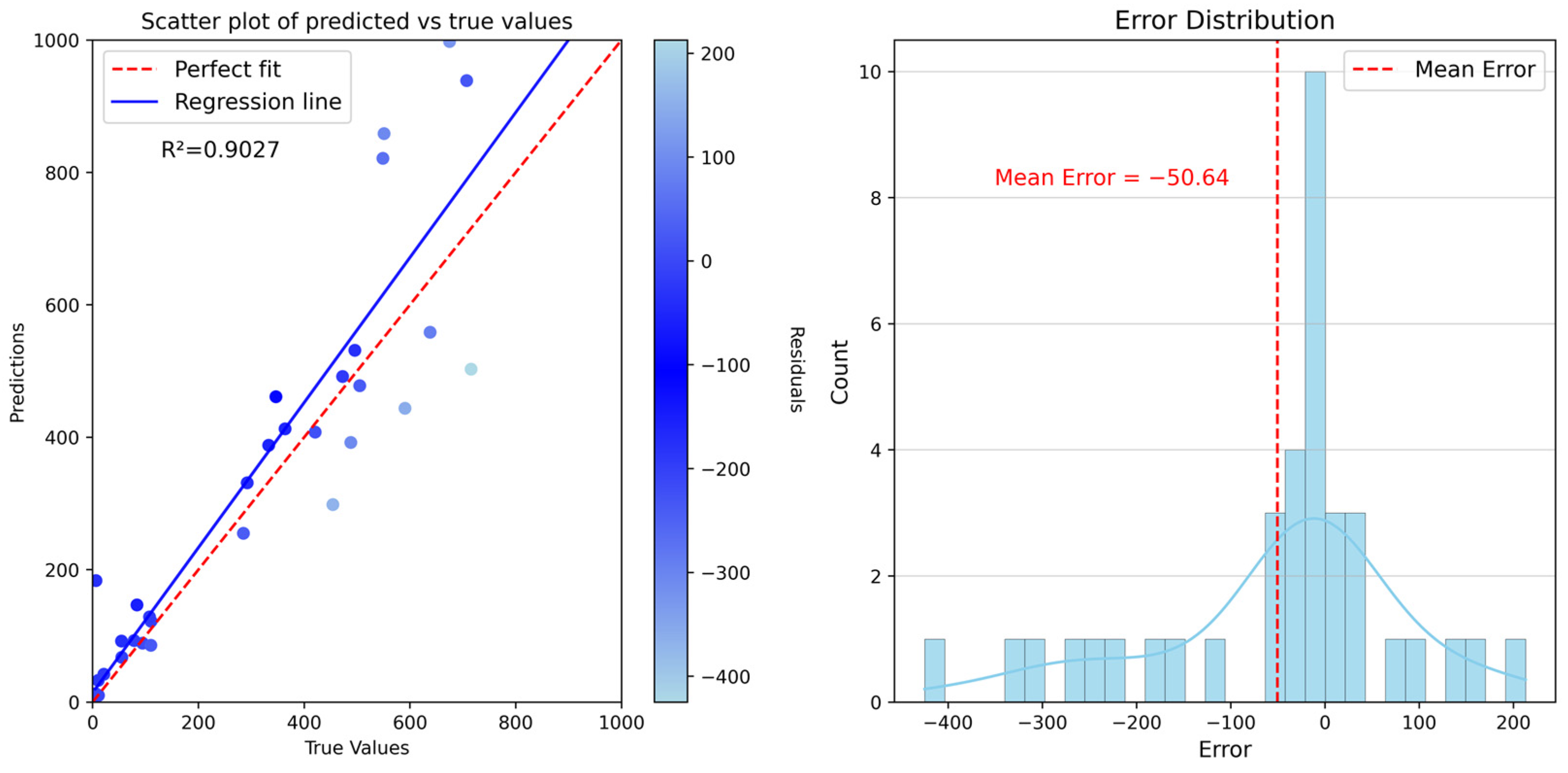
| Genetic algorithm | 0.9027 | 93.4762 | 143.3880 |
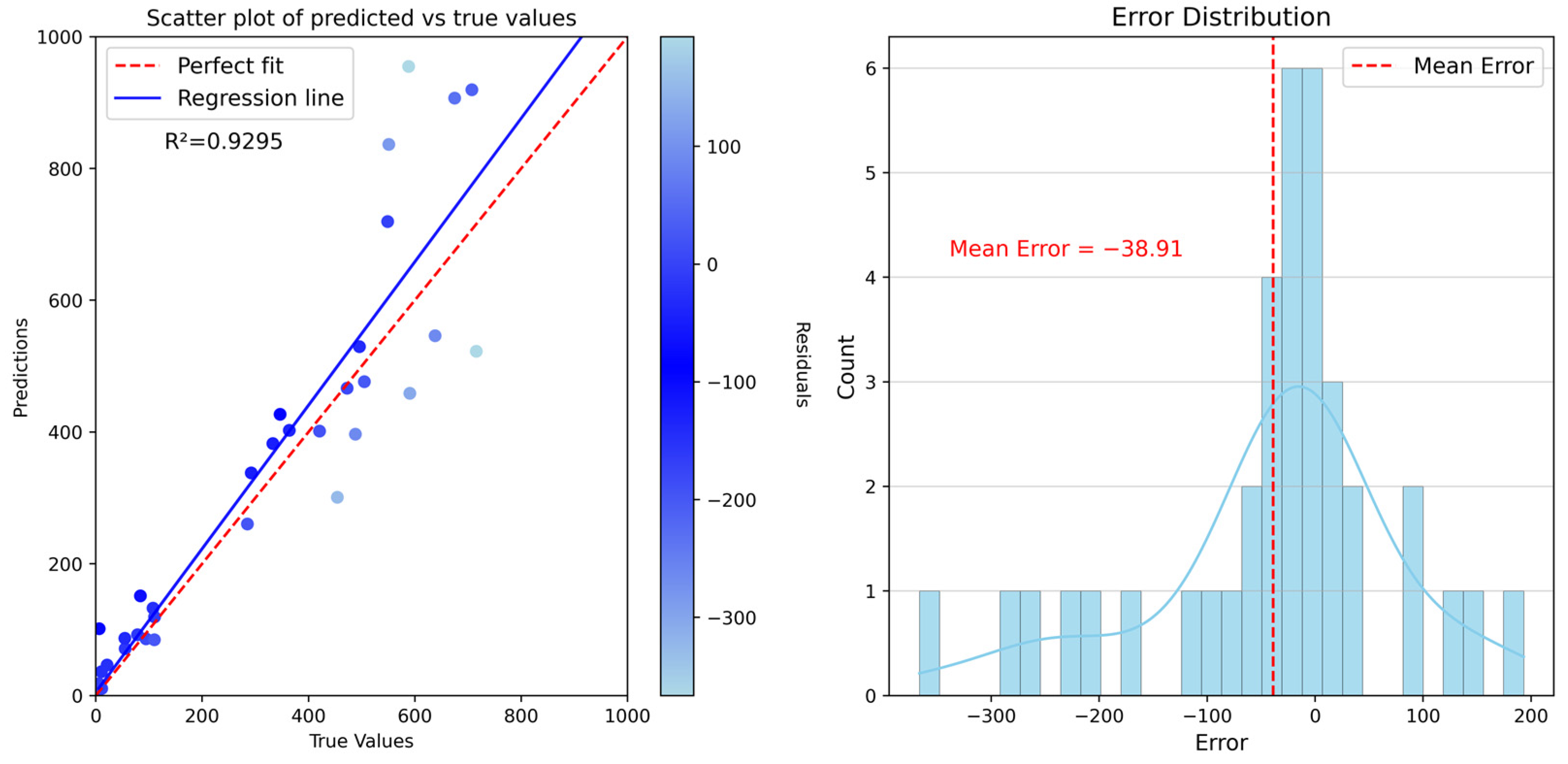
| simulated annealing algorithm | 0.9295 | 80.8391 | 122.0234 |
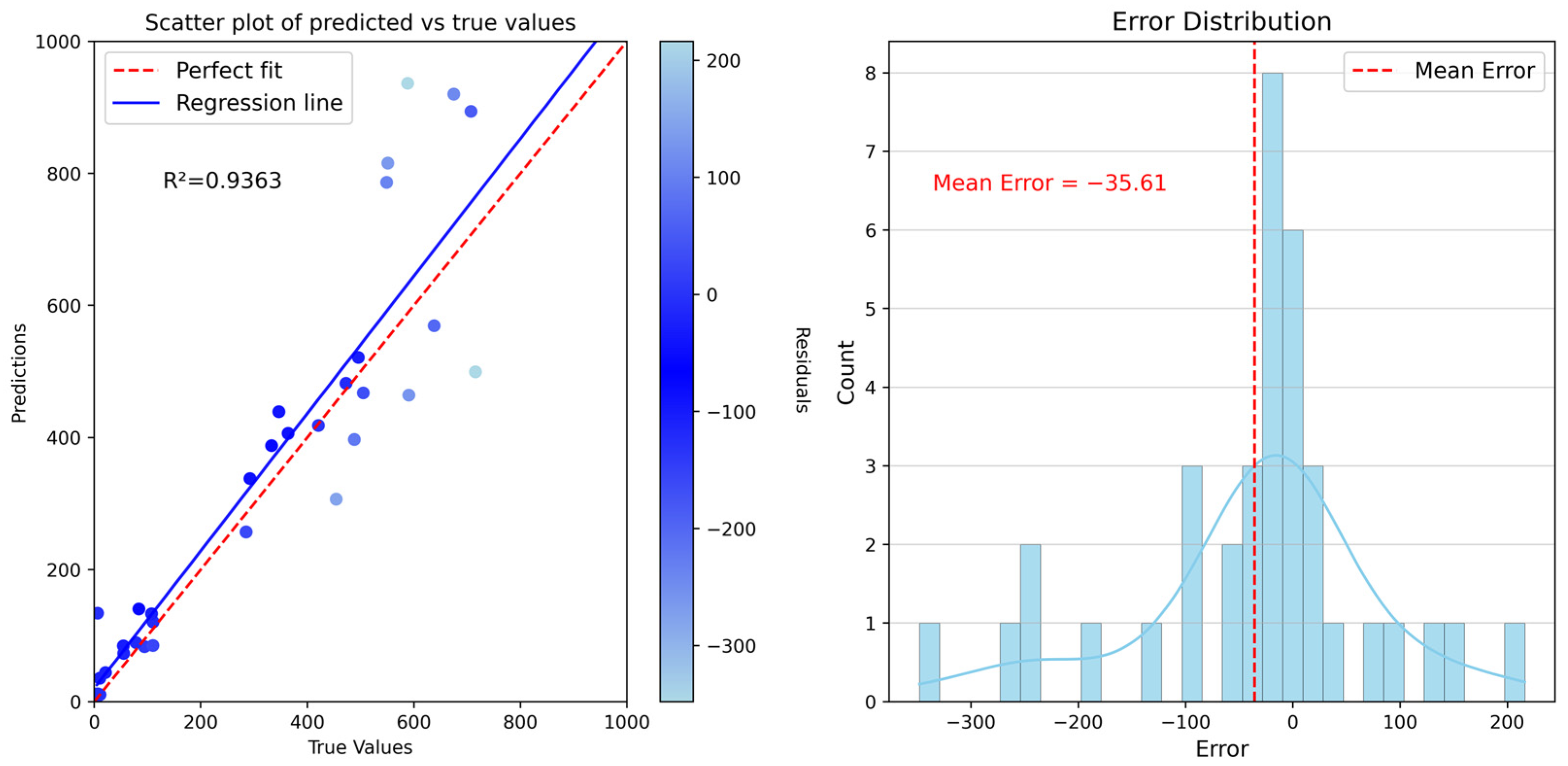
| Bayesian optimization based on Gaussian process | 0.9363 | 76.4410 | 116.0342 |
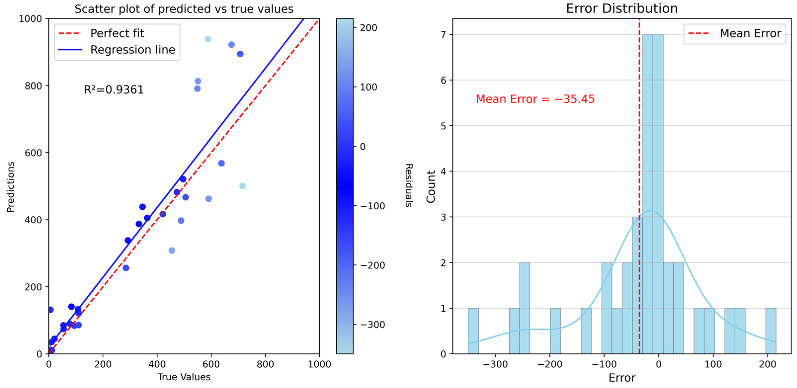
| Bayesian optimization based on gradient boosting regression trees | 0.9361 | 76.4304 | 116.1700 |
| R2 | MAE | RMSE | |
|---|---|---|---|
| LandScan | 0.3915 | 17,805.7163 | 33,634.8154 |
| GPW | 0.5384 | 13,401.9731 | 29,293.9095 |
| WorldPop | 0.6094 | 12,707.6707 | 26,947.1740 |
| RF-BOA | 0.6628 | 12,459.3926 | 25,037.1139 |
Disclaimer/Publisher’s Note: The statements, opinions and data contained in all publications are solely those of the individual author(s) and contributor(s) and not of MDPI and/or the editor(s). MDPI and/or the editor(s) disclaim responsibility for any injury to people or property resulting from any ideas, methods, instructions or products referred to in the content. |
© 2024 by the authors. Licensee MDPI, Basel, Switzerland. This article is an open access article distributed under the terms and conditions of the Creative Commons Attribution (CC BY) license (https://creativecommons.org/licenses/by/4.0/).
Share and Cite
Chen, Y.; Wang, S.; Gu, Z.; Yang, F. Modeling the Spatial Distribution of Population Based on Random Forest and Parameter Optimization Methods: A Case Study of Sichuan, China. Appl. Sci. 2024, 14, 446. https://doi.org/10.3390/app14010446
Chen Y, Wang S, Gu Z, Yang F. Modeling the Spatial Distribution of Population Based on Random Forest and Parameter Optimization Methods: A Case Study of Sichuan, China. Applied Sciences. 2024; 14(1):446. https://doi.org/10.3390/app14010446
Chicago/Turabian StyleChen, Yunzhou, Shumin Wang, Ziying Gu, and Fan Yang. 2024. "Modeling the Spatial Distribution of Population Based on Random Forest and Parameter Optimization Methods: A Case Study of Sichuan, China" Applied Sciences 14, no. 1: 446. https://doi.org/10.3390/app14010446
APA StyleChen, Y., Wang, S., Gu, Z., & Yang, F. (2024). Modeling the Spatial Distribution of Population Based on Random Forest and Parameter Optimization Methods: A Case Study of Sichuan, China. Applied Sciences, 14(1), 446. https://doi.org/10.3390/app14010446