Formation Control of Nonlinear Multi-Agent Systems with Nested Input Saturation

Featured Application

The introduced control protocol was integrated on a swarm of five commercial quadrotors to address the formation control problem.

Abstract

A decentralized robust control protocol addressing leader-follower formation control of unknown nonlinear input-constrained multi-agent systems with adaptive performance specifications is proposed in this paper. The performance characteristics predefined by the user are adaptively modified in order to comply with the actuation constraints of the agents regarding both the magnitude and the rate of the control signals, ensuring closed-loop stability. The proposed control protocol is characterized by easy gain tuning and low structural complexity which simplifies the integration to real systems. A thorough experiment involving a system of multiple quadrotors was conducted to clarify and verify the theoretical findings.

1. Introduction

1.1. Motivation

In light of the remarkable technological progress in recent decades, a substantial amount of research effort has been dedicated to the control of multi-agent systems (MAS), owing to their practical potential across diverse applications and the theoretical complexity in coordinating and controlling them [1,2,3]. The primary theoretical challenge involves controlling a multi-agent system using only the local information available to each agent and employing decentralized control laws for swarm coordination [4].

As part of cooperative control, formation control addresses the development of efficient controllers aiming to guide a fleet of agents to maintain a desired formation configuration while tracking a reference trajectory or following a designated path. Employing distributed formation control schemes for MAS becomes crucial for executing intricate cooperative missions. The aforementioned task becomes even more challenging when practical issues including actuator nonlinearities, unknown system dynamics and environmental disturbances are taken into account. Moreover, in real-time applications, there is a need for control protocols that prioritize time efficiency while avoiding excessive computational complexity. Such complexity could adversely impact system performance and even lead to instability. Despite the urge for low computational complexity algorithms, standard performance specifications have to be provided by the control laws so that the desired system response is guaranteed. Hence, the fundamental motivation for this work arises both from the practical as well as theoretical challenges outlined in this paragraph and concerns the development of a robust decentralized control strategy, capable of addressing internal and external nonlinearities and imposing performance specifications while avoiding the explosion of computational complexity.

1.2. State of the Art and Contributions

The literature on formation control of MAS demonstrates a rich amount of methodologies facilitating coordinated navigation and adaptive configurations among multiple autonomous agents. Strategies like behavior-based schemes [5,6,7], virtual structures [8,9] and leader-follower approaches [10,11,12,13,14,15] have significantly influenced the shaping of formations and the interaction control among agents. In region-based algorithms the agents move within a dynamic area, defining the desired formation shape via potential functions [16]. In ref. [17] the authors address the challenge of elliptical coverage by employing an elliptical potential function to achieve area coverage. An adaptive leader-follower formation tracking protocol for spacecraft formation was recently proposed in ref. [18], addressing limited sensing and external disturbances. This study introduces an adaptive leader-following technique for spacecraft, guaranteeing stability, connectivity maintenance, collision avoidance, and disturbance rejection within a settled time. In ref. [19] the appointed-time formation control for multiple spacecrafts under resource constraints was investigated by introducing an event-triggered protocol. Using a sliding mode manifold and output performance constraints, the authors devise a controller ensuring desired convergence and performance guarantees. Additionally, the fixed-time fault-tolerant formation control for a leader-follower heterogeneous MAS, considering actuator faults and disturbances was investigated into ref. [20]. Specifically, a finite-time performance function was introduced to ensure the convergence of formation errors within a specified time frame in combination with a distributed formation control algorithm using sliding mode control. Utilizing the digital twin framework authors in refs. [21,22] focus on a decentralized adaptive attack-resilient control scheme designed to address unbounded actuation attacks within heterogeneous MAS, ensuring the system’s resilience and stability despite adversarial disruptions.

Despite these advancements, a critical challenge persists in ensuring robust performance when confronted with input constraints. While these control strategies excel in shaping formations, they often struggle to maintain stability, convergence, and performance guarantees under real-world circumstances and limitations. In particular, actuation constraints, frequently lead to degraded tracking accuracy, stability issues, and reduced convergence rates, affecting the performance and safe operation of the MAS in practical applications. Extensive research efforts have focused on addressing these challenges within the MAS control framework. Adaptive sliding-mode control methods [23,24] and optimal control algorithms [25,26] aimed to both maintain formations and address uncertainties present in agent dynamics. Robust adaptive controllers [27], have also been introduced to counteract external disturbances, parameter uncertainties, and input nonlinearities within the control loop. Nevertheless, complex MAS, (e.g., swarms of quadrotors), often exhibit highly nonlinear behavior influenced by both internal uncertainties and external disturbances. Consequently, achieving high-performance formation tracking in such nonlinear MAS remains a fundamental challenge for researchers.

Recent advances in control methodologies have leveraged approximation techniques, driven by advancements in computational capabilities. In [28] the authors propose an adaptive fuzzy backstepping controller for the formation control of under-actuated spacecraft teams, addressing unknown nonlinearities and actuator saturation. They introduce a path-following mechanism for the leader and a follower control design based on Lyapunov theory to maintain the desired formation. Furthermore, ref. [29] proposes a neuro-adaptive leader-follower formation control scheme for autonomous surface vehicles, ensuring scalable formation sizes, while addressing uncertainties and input saturation. However, such approaches reveal certain limitations. For instance, while neuro/fuzzy approximating structures have been utilized to compensate for model uncertainties, they escalate complexity by necessitating additional adaptive parameters and computational overhead. Furthermore, the shaping of the transient and steady-state response in systems under model uncertainties and input saturation lacks systematic methods that: (i) guarantee the best achievable performance specifications, (ii) facilitate the control parameter selection and (iii) predict the steady-state behavior when input saturation is inactive.

Thus, while existing research demonstrates progress in confronting input limitations and uncertainties in MAS formation control, the challenges of ensuring robust performance and stability under actuation constraints still remain open. This highlights the need for further exploration into methodologies that offer stronger performance guarantees against input constraints, emphasizing on a more comprehensive approach to address these nonlinearities in practical scenarios. Driven by this, we build on our previous work [30] aiming at designing a novel robust scheme for controlling nonlinear MAS, considering input constraints while ensuring adaptive performance attributes. The main contributions of our work can be outlined as follows:

• In contrast to existing literature regarding MAS framework [15,17,18,19,20,23,24,25,26,27,28,29], the proposed methodology considers the conflict between output performance and input constraints both on the amplitude and rate of the control signal.
• The controller does not exploit either knowledge of the system dynamics or any disturbance observer leading to a lower complexity control scheme compared to [15,18,19,20,26,27,28,29].
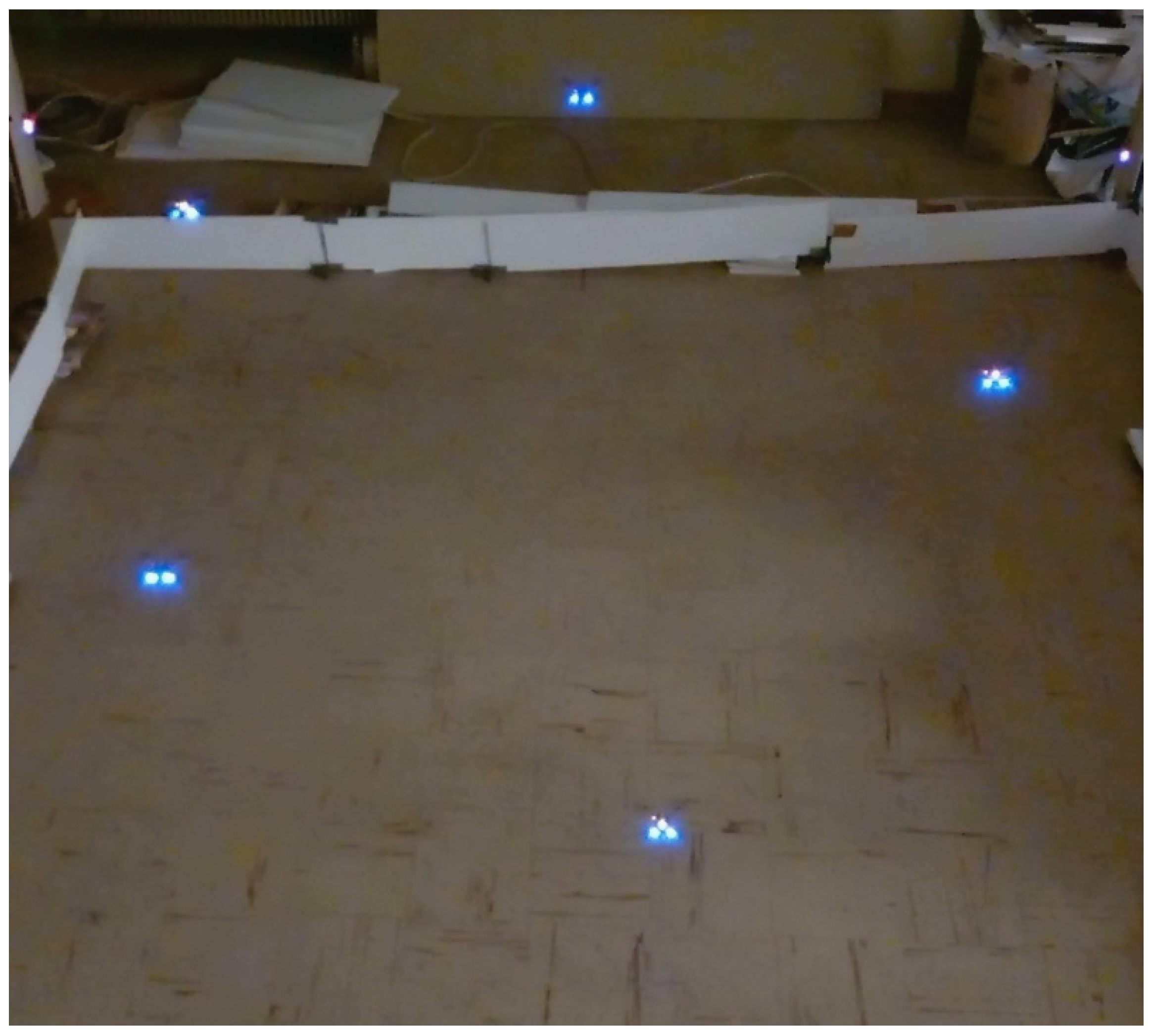
• The control protocol is decentralized with easy gain tuning, which facilitates its integration on a real robotic swarm, as illustrated in Figure 1.

The paper is structured as follows: Section 2 introduces the problem addressed in this work. Subsequently, Section 2.1 provides essential preliminary information about the PPC methodology. In Section 3.1, we formulate the neighborhood error, incorporating the system’s formation characteristics. Section 3.2 presents the design of the proposed control scheme and provides theoretical analysis for the SISO case, while Section 3.3 elaborates on the extension of the proposed controller to MIMO MAS. Section 4 presents comparative simulation results, demonstrating the superior performance of our approach compared to a well-established proportional control scheme. Moving to Section 5, we showcase experimental results highlighting the effectiveness of the proposed scenario within a real MAS setup. Finally, in Section 6, we draw conclusions from our findings.

2. Problem Formulation and Preliminaries

The system considered consists of N following agents and a leading virtual agent that generates a reference trajectory for the MAS. We assume that the agents obey the following first-order nonlinear dynamical model:

$$\begin{array}{cc}\hfill {\dot{x}}_i& =f_i\left(x_i\right)+g_i\left(x_i\right)u_i+d_i\left(t\right)\hfill \end{array}$$

(1)

$$\begin{array}{cc}\hfill {\dot{u}}_i& ={\mathrm{sat}}_{r_i}\left(a_i\left(t\right)\right),i=1,\dots ,N\hfill \end{array}$$

(2)

where $x_i\in \mathbb{R},i=1,\dots ,N$ denotes the state of each agent, $f_i,g_i:\mathbb{R}$$\to \mathbb{R},i=1,\dots ,N$ are unknown locally Lipschitz functions and $d_i:{\mathbb{R}}_{+}\to \mathbb{R},i=1,\dots ,N$ models the piecewise continuous and bounded external disturbances. The dynamic control input $u_i,i=1,\dots ,N$ will be generated through (2), which utilizes nested saturation functions to impose magnitude and rate constraints on the control signals. Hence, by properly designing the control commands $a_i\left(t\right),i=1,\dots ,N$ the control input of each agent may satisfy $|u_i|\le m_i$, $|{\dot{u}}_i|\le r_i,i=1,\dots ,N$ for some $m_i,r_i>0$ denoting the symmetrical magnitude and rate saturation levels, respectively. It should be noted that the results of the paper are extendable to arbitrary dimensions as dictated in Section 3.3.

The communication architecture of the wireless network is denoted by an undirected graph $\mathcal{G}=(\mathcal{V},\mathcal{E})$, where $\mathcal{V}=(v_1,v_2,\dots ,v_N)$ represents the vertices, and $\mathcal{E}\subseteq \mathcal{V}\times \mathcal{V}$ symbolizes the edges. Each edge indicates bidirectional information exchange between neighboring agents in the group. The neighborhood of agent i is denoted by ${\mathcal{N}}_i$ and the graph’s adjacency matrix $A=\left[A_{ij}\right]\in {\mathbb{R}}^{N\times N}$ assumes $A_{ij}=1$ if $j\in {\mathcal{N}}_i$, or $A_{ij}=0$ otherwise. Furthermore, let the degree matrix $D=\mathbf{diag}\left(\left[D_i\right]\right)\in {\mathbb{R}}^{N\times N}$ be the diagonal matrix with elements that satisfy $D_i={\sum }_{j\in {\mathcal{N}}_i}{A}_{ij}$. Consequently, the graph’s Laplacian is obtained by $L=D-A\in {\mathbb{R}}^{N\times N}$. Moreover, the state of the leader node, denoted by $v_0$, is given by $x_0:{\mathbb{R}}_{+}\to \mathbb{R}$ and it is assumed to be bounded and smooth. Note, that information about the reference trajectory is exclusively provided to a subset of the N agents. The access of the followers to the leader’s state is represented by a diagonal matrix $B=\mathbf{diag}\left([b_1,b_2,\dots ,b_N]\right)\in {\mathbb{R}}^{N\times N}$. If $b_i=1$, then the i-th agent receives state information from the leader node; conversely, if $b_i=0$, then the agent has access to the leader’s state information. Consequently, we define the augmented graph as $\overline{\mathcal{G}}=(\overline{\mathcal{V}},\overline{\mathcal{E}})$, with $\overline{\mathcal{V}}=\mathcal{V}\bigcup \left\{v_0\right\}$ and $\overline{\mathcal{E}}=\mathcal{E}\bigcup \{(v_i,v_0):b_i=1\}\subseteq \overline{\mathcal{V}}\times \overline{\mathcal{V}}$, along with the augmented set of neighbors ${\overline{\mathcal{N}}}_i=\{v_j:(v_i,v_j)\in \overline{\mathcal{E}}\},i=1,2,\dots ,N$.

We now formulate the formation control problem for the aforementioned MAS subject to limited actuation capacity, encompassing adaptive performance regarding transient and steady-state response that is confronted in this paper. Our principal goal is to devise a decentralized control strategy for the following agents of the system, assuming unknown system dynamics and external disturbances. This work aims to establish and maintain a constantly feasible formation, outlined by the desired relative offsets $d_{ij},j\in {\mathcal{N}}_i,i=1,\dots ,N$, with adaptive performance characteristics. In order to impose adaptive performance characteristics we build on the adaptive performance control technique [30], to design online adaptation laws for the user-predefined specifications (i.e., speed of convergence and steady-state error) with respect to the input limitations that inevitably prevent the accurate tracking and may put the system at risk, i.e., lead to unstable behavior. To address the previously stated problem, we establish the following assumptions:

Assumption 1.

The communication graph $\mathcal{G}$ is connected, and there exists at least one $b_i\ne 0$, $i=1,2,\dots ,N$.

Assumption 2.

The system (1) under consideration is input to state stable.

Remark 1.

Assumption 1 implies that $L+B$ forms a strictly diagonally dominant $\mathcal{M}$-matrix [31]. An $\mathcal{M}$-matrix possesses non-positive off-diagonal entries and all principal minors non-negative, ensuring the positive definiteness of $L+B$. Assumption 2 is reasonable for stabilizing input constrained systems [32]. Within the input-constrained MAS framework, characterized by strong inter-agent couplings, maintaining bounded signals for a general system is quite challenging, even if each agent initializes within a set contained within its own region of attraction.

2.1. Preliminaries on PPC

In prescribed performance control (PPC) [33], the primary aim is to achieve a specific output tracking performance, ensuring the convergence of the error to a predetermined residual set with a predefined minimum convergence rate. The approximation-free framework, introduced in [33], focuses on the difference between the measured output $y\left(t\right)$ and the desired reference trajectory $y_d\left(t\right)$, referred to as the tracking error $e\left(t\right)$. This performance is quantified by exploiting a decaying exponential function $\rho \left(t\right)=(\rho \left(0\right)-{\rho }_{\infty })exp(-\lambda t)+{\rho }_{\infty }$, characterized by parameters $\rho \left(0\right)$, ${\rho }_{\infty }$, and $\lambda$. The parameters ${\rho }_{\infty }$ and $\lambda$ represent the maximum allowable steady-state error and the convergence rate, respectively. The prescribed performance requirement demands that the tracking error $e\left(t\right)$ remains bounded within the performance envelope defined by $\rho \left(t\right)$ and $-\rho \left(t\right)$ for all $t\ge 0$ (i.e., $-\rho \left(t\right)<e\left(t\right)<\rho \left(t\right),\forall t\ge 0$). Additionally, the initial tracking error $e\left(0\right)$ is considered within the performance envelope, adhering to the condition $\rho \left(0\right)>|e(0)|$ at $t=0$.

3. Main Results

3.1. Sufficient Conditions

Owing to the incorporation of decentralized control protocols reliant on relative state information, each agent’s control law should be derived from its neighborhood error feedback:

$$e_i=\sum _{j\in {\mathcal{N}}_i}\left[A_{i,j}(x_i-x_j+d_{ij})\right]+b_i(x_i-x_0+d_{i0})$$

(3)

for $i=1,\dots ,N$ with $d_{ij},j\in {\mathcal{N}}_i$ denoting the relative inter-agent offsets that define the desired swarm formation. In addition, we define the collective neighborhood error vector as $\mathbf{e}={[e_1,\dots ,e_N]}^T\in {\mathbb{R}}^N$. Leveraging on the graph topology and through straightforward algebraic manipulations, this vector can be expressed as:

$$\mathbf{e}=\left(L+B\right)\left(\mathbf{x}-{\mathbf{x}}_0+\mathbf{d}\right)$$

(4)

where $\mathbf{x}=[x_1,\dots ,x_N]\in {\mathbb{R}}^N$ represents the collective state vector of the MAS, with ${\mathbf{x}}_0={[x_0,\dots ,x_0]}^T\in {\mathbb{R}}^N$ and

$$\mathbf{d}={(L+B)}^{-1}{\left[\sum _{j\in {\mathcal{N}}_1}\left(A_{1,j}{d}_{1j}\right)+b_1{d}_{10},\dots ,\sum _{j\in {\mathcal{N}}_N}\left(A_{N,j}{d}_{Nj}\right)+b_N{d}_{N0}\right]}^T$$

corresponds to the relative offset of the i-th agent with respect to the leader within the desired formation configuration. Consequently, the formation is aligned with the leader’s state, hence it is achieved when each agent’s state $x_i$ with respect to the leader state $x_0$ maintains its respective offset ${\mathbf{d}}_i$, $i=1,\dots ,N$. Introducing the disagreement formation variable as $\mathbf{q}={[q_1,\dots ,q_N]}^T=\mathbf{x}-{\mathbf{x}}_0-\mathbf{d}$, the formation control objective is met when the disagreement errors $s_i$ approach an arbitrarily small set around the origin for all $i=1,\dots ,N$. However, $q_i$ represents global quantities and cannot be measured distributedly based on the local intercourse specifications, as they utilize information directly sourced from the leader. However, due to the non-singularity of $L+B$ as a result of Assumption 1, we arrive at:

$$|\mathbf{q}|\le \frac{|\mathbf{e}|}{{\lambda }_{min}(L+B)}$$

(5)

where ${\lambda }_{min}(L+B)$ corresponds to the smallest singular value of $L+B$.

Remark 2.

From (5) it is concluded that the error vector $\mathbf{e}$ can serve as a reliable measure of the formation control problem. Thus, transient and steady-state bounds on the neighborhood errors $e_i$, $i=1,\dots ,N$ can be directly mapped into constraints on the disagreement formation metrics $q_i$, $i=1,\dots ,N$. This leads to the conclusion that solving the adaptive performance control problem for all neighborhood errors $e_i$ directly resolves the formation control problem of (1). Specifically, as dictated by (5), ensuring $|e_i\left(t\right)|<{\rho }_i\left(t\right)$, for all $t\ge 0$ and $i=1,\dots ,N$, with ${\rho }_i\left(t\right)$ denoting a performance function to be designed, explicitly constrain the disagreement errors $q_i$, $i=1,\dots ,N$ within the compact sets ${\mathcal{Q}}_i:=\{q_i\in \mathbb{R}:|q_i|\le \frac{{\overline{\rho }}_i}{{\lambda }_{min}(L+B)}\}$ where ${\overline{\rho }}_i$ denotes an upper bound on ${\rho }_i\left(t\right)$. Yet, ${\lambda }_{min}(L+B)$ remains a global parameter, rendering it impractical for exploitation within decentralized control methodologies to directly enforce specific limits on $\mathbf{q}$ through Equation (5). To address this challenge, a decentralized estimation algorithm [34] could be initially employed to estimate ${\lambda }_{min}(L+B)$.

3.2. Decentralized Controller Design

In this section, we present an approximation-free decentralized dynamic control scheme that guarantees $|e_i\left(t\right)|<{\rho }_i\left(t\right),i=1,\dots ,N$ and appropriately adapts the magnitude of ${\rho }_i\left(t\right)$ to incorporate both the output (performance) and input (actuation) constraints. This eventually leads to the solution of the robust formation control problem with adaptive performance for the input-constrained MAS. To account for system constraints, we introduce a smooth saturation function $\sigma (\chi ,\overline{\sigma }):\mathbb{R}\to [-\overline{\sigma },\overline{\sigma }]$, where $\overline{\sigma }>0$ represents the saturation level. Within this context, we select the saturation function as:

$$\begin{array}{c}\hfill \sigma (\chi ,\overline{\sigma })=\left\{\begin{array}{cc}\chi \hfill & \mathrm{if}|\chi |<\overline{\sigma }-\beta \hfill \\ p\left(\chi \right)\hfill & \mathrm{if}|\chi |\in [\overline{\sigma }-\beta ,\overline{\sigma }+\beta ]\hfill \\ s_{\chi }\overline{\sigma }\hfill & \mathrm{if}|\chi |>\overline{\sigma }+\beta \hfill \end{array}\right.\end{array}$$

where:

$$p\left(\chi \right)=-\frac{1}{4\beta }\left({\chi }^2-2s_{\chi }(\overline{\sigma }+\beta )\chi +{(s_{\chi }\overline{\sigma }-s_{\chi }\beta )}^2\right)$$

with $s_{\chi }$ denoting the $\mathrm{sign}$ of $\chi$ and $\beta ={10}^{-6}$ serves as a small smoothing parameter. The design methodology of the proposed controller is elaborated as follows:

Step 1. The reference control signal is given by:

$$\begin{array}{cc}\hfill u_{d_i}\left(t\right)& =-k_{i,1}T\left(\frac{e_i\left(t\right)}{{\rho }_{i,1}\left(t\right)}\right),i=1,\dots ,N\hfill \end{array}$$

(6)

with $k_{i,1}>0$ and $T:(-1,1)\to (-\infty ,\infty )$ denoting a smooth error transformation function. In this work, we select the mapping $T\left(\chi \right)=\frac{1}{2}ln\left(\frac{1+\chi }{1-\chi }\right)$. Owing to the definition of T the initial value of the performance ${\rho }_{i,1}\left(t\right)$ should be selected to satisfy $|e_i\left(0\right)|<{\rho }_1\left(0\right)$.

Step 2. The adaptive performance law that incorporates the output performance requirements and the input magnitude saturation is obtained by:

$${\dot{\rho }}_{i,1}=\left[\frac{\sigma (u_{d_i}\left(t\right),m_i)-u_{d_i}\left(t\right)}{e_i\left(t\right)}-{\lambda }_{i,1}\left(1-\frac{{\rho }_{i,1}^{\infty }}{{\rho }_{i,1}\left(t\right)}\right)\right]{\rho }_{i,1}\left(t\right),i=1,\dots ,N$$

(7)

where ${\lambda }_{i,1}$, ${\rho }_{i,1}^{\infty }>0$ correspond to the desired convergence rate and the maximum allowable steady-state error, respectively.

Step 3. The reference control rate signal is given by:

$$\begin{array}{cc}\hfill a\left(t\right)& =-k_{i,2}T\left(\frac{u_i\left(t\right)-\sigma (u_{d_i}\left(t\right),m_i)}{{\rho }_{i,2}\left(t\right)}\right),i=1,\dots ,N\hfill \end{array}$$

(8)

with $k_{i,2}>0$.

Step 4. Similar to (7), the adaptive performance law that encompasses rate saturation on the control signal is obtained by:

$$\begin{array}{c}\hfill {\dot{\rho }}_{i,2}=\left[\frac{\sigma (a_i\left(t\right),r_i)-a_i\left(t\right)}{u_i\left(t\right)-\sigma (u_{d_i}\left(t\right),m_i)}-{\lambda }_{i,2}\left(1-\frac{{\rho }_{i,2}^{\infty }}{{\rho }_{i,2}\left(t\right)}\right)\right]{\rho }_{i,2}\left(t\right),i=1,\dots ,N\end{array}$$

(9)

with ${\lambda }_{i,2}$, ${\rho }_{i,2}^{\infty }>0$ and $|u_i\left(t\right)-\sigma (u_{d_i}\left(t\right),m_i)|<{\rho }_2\left(0\right)$. Thus, the dynamic decentralized controller, subjected to both magnitude and slew-rate saturation, is obtained by:

$${\dot{u}}_i=\sigma (a_i\left(t\right),r_i),u_i\left(0\right)\in [-m_i,m_i]$$

(10)

for $i=1,\dots ,N$.

Remark 3.

Both adaptive laws (7) and (9) consist of two components. The second term, negative in nature, incorporates the predefined performance attributes and represents the conventional performance function $\rho \left(t\right)=(\rho \left(0\right)-{\rho }_{\infty })exp(-\lambda t)+{\rho }_{\infty }$. Conversely, the first term, non-negative and inactive under normal plant operation, i.e., when the control signal is away from saturation, triggers when control signals $u_{d_i}\left(t\right),a_i\left(t\right),i=1,\dots ,N$ reach their saturation level. Its activation widens the corresponding performance boundaries based on the difference between the desired and saturated control signals, ensuring the boundedness of all loop signals. Notably, as the second term in (7) and (9) becomes dominant, the relaxation of performance boundaries halts, and once the saturation ceases then the performance envelope retrieves its predefined form.

Remark 4.

The proposed control protocol operates in a decentralized manner, where each agent solely relies on local relative state information within its neighborhood, expressed in a common frame, to compute its individual control signal. Notably, this protocol does not utilize any knowledge of system dynamics or disturbances. Moreover, it does not employ approximation structures such as neural networks or fuzzy systems to acquire such insights. Moreover, generating the control signal does not necessitate intricate calculations, simplifying its implementation. Thus, the proposed formation protocol not only remains decentralized but also showcases low structural complexity.

Theorem 1.

Consider system (1)) obeying Assumptions 1 and 2. The proposed adaptive decentralized control protocol (6)–(10) ensures the boundedness of all loop signals and guarantees:

$$|e_i\left(t\right)|<{\rho }_{i,1}\left(t\right),i=1,\dots ,N$$

(11)

for all $t\ge 0$.

Proof. 

Let us first define the normalized tracking error vectors:

$$\begin{array}{cc}\hfill {\xi }_1& :={\left[\begin{array}{c}\frac{e_1\left(t\right)}{{\rho }_{1,1}\left(t\right)},\dots ,\frac{e_N\left(t\right)}{{\rho }_{N,1}\left(t\right)}\end{array}\right]}^T\hfill \end{array}$$

(12)

$$\begin{array}{cc}\hfill {\xi }_2& :={\left[\begin{array}{c}\frac{u_1\left(t\right)-\sigma (u_{d_1}\left(t\right),m_1)}{{\rho }_{1,2}\left(t\right)},\dots ,\frac{u_N\left(t\right)-\sigma (u_{d_N}\left(t\right),m_N)}{{\rho }_{N,2}\left(t\right)}\end{array}\right]}^T\hfill \end{array}$$

(13)

Notice from (4) and (12) that the state vector can be written as $\mathbf{x}={(L+B)}^{-1}{\rho }_1\left(t\right){\xi }_1\left(t\right)+{\mathbf{x}}_0-\mathbf{d}$ with ${\rho }_1\left(t\right)=\mathbf{diag}\left([{\rho }_{1,1}\left(t\right),\dots ,{\rho }_{N,1}\left(t\right)]\right)$. Differentiating ${\xi }_1\left(t\right)$ with respect to time and substituting (1), (2), (4) and (6)–(10) as well as adding and subtracting $(L+B)g\left(\mathbf{x}\right)\sigma (u_d\left(t\right),m)$ we get:

$$\begin{array}{cc}\hfill {\dot{\xi }}_1=& {\left({\rho }_1\left(t\right)\right)}^{-1}[(L+B)(f\left(\mathbf{x}\right)+g\left(\mathbf{x}\right)\tilde{u}\left({\xi }_1\right)+d\left(t\right)-{\dot{\mathbf{x}}}_0)\hfill \\ & +{\xi }_1\left(t\right){\lambda }_1({\rho }_1\left(t\right)-{\rho }_1^{\infty })+((L+B)g\left(\mathbf{x}\right)-1)\sigma (u_{d_i}\left(t\right),m_i)-k_1{ϵ}_1\left({\xi }_1\right)]\hfill \end{array}$$

(14)

where:

$$\begin{array}{cc}\hfill f\left(\mathbf{x}\right)& ={[f_1\left(x_1\right),\dots ,f_N\left(x_N\right)]}^T\hfill \\ \hfill g\left(\mathbf{x}\right)& =\mathbf{diag}\left([g_1\left(x_1\right),\dots ,g_N\left(x_N\right)]\right)\hfill \\ \hfill \tilde{u}\left({\xi }_1\right)& ={[u_1\left(t\right)-\sigma (u_{d_1}\left(t\right),m_1),\dots ,u_N\left(t\right)-\sigma (u_{d_N}\left(t\right),m_1)]}^T\hfill \\ \hfill \sigma (u_d\left(t\right),m)& ={[\sigma (u_{d_1}\left(t\right),m_1),\dots ,\sigma (u_{d_N}\left(t\right),m_N)]}^T\hfill \\ \hfill {ϵ}_1\left({\xi }_1\right)& ={\left[T\left(\frac{e_1\left(t\right)}{{\rho }_{1,1}\left(t\right)}\right),\dots ,T\left(\frac{e_N\left(t\right)}{{\rho }_{N,1}\left(t\right)}\right)\right]}^T\hfill \\ \hfill {\lambda }_1& =\mathbf{diag}\left([{\lambda }_{1,1},\dots ,{\lambda }_{N,1}]\right)\hfill \\ \hfill {\rho }_1^{\infty }& =\mathbf{diag}\left([{\rho }_{1,1}^{\infty },\dots ,{\rho }_{N,1}^{\infty }]\right)\hfill \\ \hfill k_1& =\mathbf{diag}\left([k_{1,1},\dots ,k_{N,1}]\right).\hfill \end{array}$$

Following the same reasoning the dynamics of ${\xi }_2$ may be written as:

$$\begin{array}{cc}\hfill {\dot{\xi }}_2=& {\left({\rho }_2\left(t\right)\right)}^{-1}\left(-k_1{\sigma }^{\prime }(u_d\left(t\right),m){\dot{\xi }}_1{\nabla }_{{\xi }_1}{ϵ}_1+{\xi }_2\left(t\right){\lambda }_2({\rho }_2\left(t\right)-{\rho }_2^{\infty })-k_2{ϵ}_2\left({\xi }_2\right)\right)\hfill \end{array}$$

(15)

where:

$$\begin{array}{cc}\hfill {\sigma }^{\prime }(u_d\left(t\right),m)& ={\left[\frac{d\sigma (u_{d_1}\left(t\right),m_1)}{dt},\dots ,\frac{d\sigma (u_{d_N}\left(t\right),m_N)}{dt}\right]}^T\hfill \\ \hfill {ϵ}_2\left({\xi }_2\right)& ={\left[T\left(\frac{u_1\left(t\right)-\sigma (u_{d_1}\left(t\right),m_1)}{{\rho }_{1,2}\left(t\right)}\right),\dots ,T\left(\frac{u_N\left(t\right)-\sigma (u_{d_N}\left(t\right),m_N)}{{\rho }_{N,2}\left(t\right)}\right)\right]}^T\hfill \\ \hfill {\nabla }_{{\xi }_1}{ϵ}_1& =\mathbf{diag}\left(\left[\frac{1}{1-{\xi }_{1,1}^2},\dots ,\frac{1}{1-{\xi }_{1,N}^2}\right]\right)\hfill \\ \hfill {\rho }_2\left(t\right)& =\mathbf{diag}\left([{\rho }_{1,2}\left(t\right),\dots ,{\rho }_{N,2}\left(t\right)]\right)\hfill \\ \hfill {\lambda }_2& =\mathbf{diag}\left([{\lambda }_{1,2},\dots ,{\lambda }_{N,2}]\right)\hfill \\ \hfill {\rho }_2^{\infty }& =\mathbf{diag}\left([{\rho }_{1,2}^{\infty },\dots ,{\rho }_{N,2}^{\infty }]\right)\hfill \\ \hfill k_2& =\mathbf{diag}\left([k_{1,2},\dots ,k_{N,2}]\right).\hfill \end{array}$$

Next consider the positive definite and radially unbounded $\mathrm{Lyapunov}$ function candidate $L=\frac{1}{2}{ϵ}_1^T{ϵ}_1+\frac{1}{2}{ϵ}_2^T{ϵ}_2$. By differentiating L with respect to time, we get:

$$\begin{array}{cc}\hfill \dot{L}=& {ϵ}_1^T{\nabla }_{{\xi }_1}{ϵ}_1{\left({\rho }_1\left(t\right)\right)}^{-1}[(L+B)(f\left(\mathbf{x}\right)+g\left(\mathbf{x}\right)\tilde{u}\left({\xi }_1\right)+d\left(t\right)-{\dot{\mathbf{x}}}_0)\hfill \\ & +{\xi }_1\left(t\right){\lambda }_1({\rho }_1\left(t\right)-{\rho }_1^{\infty })+((L+B)g\left(\mathbf{x}\right)-1)\sigma (u_d\left(t\right),m)-k_1{ϵ}_1\left({\xi }_1\right)]\hfill \\ & +{ϵ}_2^T{\nabla }_{{\xi }_2}{ϵ}_2{\left({\rho }_2\left(t\right)\right)}^{-1}\left(-k_1{\sigma }^{\prime }(u_d\left(t\right),m){\dot{\xi }}_1{\nabla }_{{\xi }_1}{ϵ}_1+{\xi }_2\left(t\right){\lambda }_2({\rho }_2\left(t\right)-{\rho }_2^{\infty })-k_2{ϵ}_2\left({\xi }_2\right)\right)\hfill \end{array}$$

(16)

with ${\nabla }_{{\xi }_2}{ϵ}_2=\mathbf{diag}\left(\left[\frac{1}{1-{\xi }_{2,1}^2},\dots ,\frac{1}{1-{\xi }_{2,N}^2}\right]\right)$. Note, that $\tilde{u}\left({\xi }_1\right)$ is bounded due to the magnitude saturation, decoupling the boundedness of ${\xi }_1$ and ${\xi }_2$. Next owing to the continuity of the unknown dynamics of (1), the boundedness of the external disturbances $d\left(t\right)$ and ${\mathbf{x}}_0$, the saturation limits $m_i,r_i,i=1,\dots ,N$ as well as exploiting Assumption 2 which implies the boundedness of $\mathbf{x},{\rho }_1\left(t\right),{\rho }_2\left(t\right)$ [30] we conclude the existence of some positive constants $F_1,F_2$ such that:

$$\begin{array}{cc}\hfill & \parallel (L+B)(f\left(\mathbf{x}\right)+g\left(\mathbf{x}\right)\tilde{u}\left({\xi }_1\right)+d\left(t\right)-{\dot{\mathbf{x}}}_0)\hfill \\ & +{\xi }_1\left(t\right){\lambda }_1({\rho }_1\left(t\right)-{\rho }_1^{\infty })+((L+B)g\left(\mathbf{x}\right)-1)\sigma (u_d\left(t\right),m)\parallel \le F_1\hfill \\ \hfill & \parallel -k_1{\sigma }^{\prime }(u_d\left(t\right),m){\dot{\xi }}_1{\nabla }_{{\xi }_1}{ϵ}_1+{\xi }_2\left(t\right){\lambda }_2({\rho }_2\left(t\right)-{\rho }_2^{\infty })\parallel \le F_2\hfill \end{array}$$

Additionally, the matrices ${\nabla }_{{\xi }_1}{ϵ}_1,{\left({\rho }_1\left(t\right)\right)}^{-1},{\nabla }_{{\xi }_2}{ϵ}_2,{\left({\rho }_2\left(t\right)\right)}^{-1},(L+B)$ are positive definite thus $\dot{L}$ becomes negative whenever $\parallel {ϵ}_1\parallel >\frac{F_1}{min\left\{k_{i,1}\right\}}$ and $\parallel {ϵ}_2\parallel >\frac{F_2}{min\left\{k_{i,2}\right\}}$. Moreover, considering the initial fulfillment of performance constraints, the initial values of ${ϵ}_1,{ϵ}_2$ are well-defined. Thus, the transformed errors ${ϵ}_1,{ϵ}_2$ are uniformly ultimately bounded. Consequently, the performance criteria, as dictated by inequality (11), are consistently met over time, ensuring adaptive performance specifications. Furthermore, all signals within the closed-loop system remain bounded, thereby concluding the proof. □

Remark 5.

Theorem 1 ensures the boundedness of the neighborhood error $\mathbf{e}$ by establishing a compromise between output specifications and input limitations. However, in the absence of saturation, the system rapidly reverts to its predetermined performance characteristics exponentially. Therefore, it can be deduced that when amplitude saturation is inactive (i.e., ${\dot{\rho }}_{i,1}\left(t\right)=-{\lambda }_{i,1}({\rho }_{i,1}\left(t\right)-{\rho }_{i,1}^{\infty }))$, the disagreement formation variable $\mathbf{q}$ converges to the compact set ${\mathcal{Q}}_i^{\infty }:=\left\{q_i\in \mathbb{R}:|q_i|\le \frac{{\rho }_i^{\infty }}{{\lambda }_{min}(L+B)}\right\},i=1,\dots ,N$ with an exponential rate of at least $exp(-{\lambda }_{i,1}t)$. Consequently, in this scenario, the performance bound on $q_i\left(t\right)i=1,\dots ,N$, i.e., ${\overline{q}}_i$, can be imposed by selecting ${\rho }_i^{\infty }={\widehat{\lambda }}_{min}(L+B){\overline{q}}_i,i=1,\dots ,N$, where ${\widehat{\lambda }}_{min}(L+B)$ is the result of a decentralized connectivity estimation algorithm [34].

Remark 6.

Note, that the performance specifications for the closed-loop MAS are determined by the evolution of ${\rho }_{i,1}\left(t\right)i=1,\dots ,N$. Nevertheless, in the presence of magnitude and rate saturation, the performance constraints are inevitably relaxed to ensure the boundedness of the closed-loop signals. The extent of relaxation is contingent on the control gains $k_{i,1},i=1,\dots ,N$. Moreover, the fluctuation of the performance envelope relies on the control tracking error $u_i\left(t\right)-\sigma (u_{d_i}\left(t\right),m_i)$, as articulated in Theorem 1. Therefore, a quick convergence of $u_i\left(t\right)\to \sigma (u_{d_i}\left(t\right),m_i)$ is desirable and can be achieved by opting for relatively higher values for ${\lambda }_{i,2}$. However, large gains $k_{i,j},i=1$, $\dots ,N,j=1,2$ might lead to an excessive relaxation of the performance functions (7) and (9), resulting in an unnecessary deterioration in tracking performance owing to faster saturation of (6) and (10). On the other hand, lower gain values may result in oscillatory behavior within performance boundaries, an issue mitigated by elevating these values at the expense of increased control effort. Similarly, model uncertainties and external disturbances can affect the closed-loop response as they affect the upper bounds of the reference inputs $u_{d_i}\left(t\right)$ by regulating the magnitude of $F_1$. While the latter inevitably influences the MAS performance, the boundedness of the closed-loop signals is ensured owing to the adaptive performance mechanisms (7) and (9). This underscores the robustness of the proposed control protocol against model uncertainties and external disturbances.

3.3. Extension to Multi-Input Multi-Output MASs

The M-dimensional agent is described by:

$$\begin{array}{cc}\hfill {\dot{\zeta }}_i& =f_i\left({\zeta }_i\right)+G_i\left({\zeta }_i\right)u_i+d_i\left(t\right)\hfill \\ \hfill {\dot{u}}_i& ={\mathrm{sat}}_r\left(a_i\left(t\right)\right),i=1,\dots ,N\hfill \end{array}$$

(17)

where ${\zeta }_i\in {\mathbb{R}}^M$ denote the sate of each agent, $u_i\in {\mathbb{R}}^M$ are the control inputs, the functions $f_i:{\mathbb{R}}^M\to {\mathbb{R}}^M$, $G_i:{\mathbb{R}}^M\to {\mathbb{R}}^{M\times M}$, $d_i:{\mathbb{R}}^{+}\to {\mathbb{R}}^M$ for $i=1,\dots ,N$ denotes the nonlinear terms of the system and the external disturbances, respectively, and ${\zeta }_0:{\mathbb{R}}^{+}\to {\mathbb{R}}^M$ corresponds to the state of the leader. To solve the input-constrained formation control problem with adaptive performance we follow a similar approach as in Section 3.2, given a controllability assumption on the positive (or negative) definiteness of the matrices $G_i(·)$ for $i=1,\dots ,N$.

Specifically, the neighborhood error feedback is defined as:

$$e_i=\sum _{j\in {\mathcal{N}}_i}{a}_{ij}({\zeta }_i-{\zeta }_j+d_{ij})+b_i({\zeta }_i-{\zeta }_0+d_{i0})\in {\mathbb{R}}^M$$

for $i=1,\dots ,N$. Using the Kronecker product ⊗, we derive the overall neighborhood error vector:

$$\mathbf{e}={\left[e_1^T,\dots ,e_N^T\right]}^T=\left((L+B)\otimes I_M\right)(\zeta -{\zeta }_0+\mathbf{d})$$

where $\zeta ={\left[{\zeta }_1^T,\dots ,{\zeta }_N^T\right]}^T\in {\mathbb{R}}^{NM}$ represents the overall state vector, ${\zeta }_0={\left[{\zeta }_0^T,\dots ,{\zeta }_0^T\right]}^T\in {\mathbb{R}}^{NM}$, and $\mathbf{d}$ denotes relative offsets with respect to the leader, as dictated by the desired formation. Adopting the proposed control protocol (6)–(10), element-wise for each neighborhood error $e_i\left(t\right)$ it can be easily verified that the decentralized control scheme presented in

Table 1. Decentralized control protocol for MIMO MASs.

Control Protocol
$u_{d_i}\left(t\right)=-k_i^1{\left[T\left(\frac{e_{i,1}\left(t\right)}{{\rho }_{i,1}^1\left(t\right)}\right),\dots ,T\left(\frac{e_{i,M}\left(t\right)}{{\rho }_{i,M}^1\left(t\right)}\right)\right]}^T,k_i^1>0$
$a_i\left(t\right)=-k_i^2{\left[T\left(\frac{u_{i,1}\left(t\right)-\sigma (u_{d_{i,1}}\left(t\right),m_{i,1})}{{\rho }_{i,1}^2\left(t\right)}\right),\dots ,T\left(\frac{u_{i,M}\left(t\right)-\sigma (u_{d_{i,M}}\left(t\right),m_{i,M})}{{\rho }_{i,M}^2\left(t\right)}\right)\right]}^T,k_i^2>0$
${\dot{\rho }}_i^1={\left[\left(\frac{\sigma (u_{d_{i,1}}\left(t\right),m_{i,1})-u_{d_{i,1}}\left(t\right)}{e_{i,1}\left(t\right)}-{\lambda }_{i,1}^1\left(1+\frac{{\rho }_{i,1}^{1,\infty }}{{\rho }_{i,1}^1\left(t\right)}\right)\right){\rho }_{i,1}^1\left(t\right),\dots ,\left(\frac{\sigma (u_{d_{i,M}}\left(t\right),m_{i,M})-u_{d_{i,M}}\left(t\right)}{e_{i,M}\left(t\right)}-{\lambda }_{i,M}^1\left(1+\frac{{\rho }_{i,M}^{1,\infty }}{{\rho }_{i,M}^1\left(t\right)}\right)\right){\rho }_{i,M}^1\left(t\right)\right]}^T$
${\dot{\rho }}_i^2={\left[\left(\frac{\sigma (a_{i,1}\left(t\right),r_{i,1})-a_{i,1}\left(t\right)}{u_{i,1}\left(t\right)-\sigma (u_{d_{i,1}}\left(t\right),m_{i,1})}-{\lambda }_{i,1}^2\left(1+\frac{{\rho }_{i,1}^{2,\infty }}{{\rho }_{i,1}^2\left(t\right)}\right)\right){\rho }_{i,1}^2\left(t\right),\dots ,\left(\frac{\sigma (a_{i,M}\left(t\right),r_{i,M})-a_{i,M}\left(t\right)}{u_{i,M}\left(t\right)-\sigma (u_{d_{i,M}}\left(t\right),m_{i,M})}-{\lambda }_{i,M}^2\left(1+\frac{{\rho }_{i,M}^{2,\infty }}{{\rho }_{i,M}^2\left(t\right)}\right)\right){\rho }_{i,M}^2\left(t\right)\right]}^T$

ensures $|e_{ij}\left(t\right)|<{\rho }_{ij}^1\left(t\right)$ for all $t\ge 0$, $i=1,\dots ,N$, and $j=1,\dots ,M$, as well as boundedness of all closed-loop signals.

4. Comparative Simulation Results

In this section we present comparative simulation results in order to illustrate the superiority of the proposed control scheme against a well-established formation control algorithm described in ref. [35]. In this simulation scenario, we consider the formation control problem of five planar agents described by the following nonlinear dynamical model:

$$\begin{array}{c}\hfill \left[\begin{array}{c}{\dot{x}}_i\\ {\dot{y}}_i\end{array}\right]=\left[\begin{array}{c}0.5x_i{y}_i+exp(-x_i^2-y_i^2)\\ 0.1x_i^2-0.05y_i^2+sin\left(x_i{y}_i\right)\end{array}\right]+\left[\begin{array}{c}1+0.3sin\left(x_i\right)\\ 1+0.45cos\left(x_i\right)\end{array}\right]u_i+d_i\left(t\right)\end{array}$$

with $u_i={[u_{x,i},u_{y,i}]}^T\in [-1.2,1.2]\times [-1.2,1.2]$ and $d_i\left(t\right)={[cos\left(2t\right),-sin\left(2.5t\right)]}^T$ for all $i=1,\dots ,5$. The aim of this paradigm is to achieve a regular pentagon formation while the swarm dynamically tracks a reference trajectory set by a virtual leader centered within the formation. The reference trajectory is circular and it is given as $x_r=cos\left(0.2t\right),$ $y_r=sin\left(0.2t\right)$ for $t\in [0,25]$. The control parameters for the proposed scheme were chosen as $k_{l,i}^1=0.5,k_{l,i}^2=2,{\lambda }_{l,i}^1=0.5,{\lambda }_{l,i}^2=1,{\rho }_{l,i}^{1,\infty }=0.1,{\rho }_{l,i}^{2,\infty }=0.1,l\in \{x,y\},i=1,\dots ,5$ with ${\dot{u}}_i\in [-5,5]\times [-5,5],i=1,\dots ,5$. For the scheme of [35] the gains were chosen with fine tuning as $k_i=1.15,i=1,\dots 5$. Moreover, the adjacency matrix $\mathcal{A}$ of the communication graph and the matrix B are given by:

$$\begin{array}{cc}\hfill \mathcal{A}& =\left[\begin{array}{ccccc}0& 1& 1& 0& 0\\ 1& 0& 0& 1& 0\\ 1& 0& 0& 0& 1\\ 0& 1& 0& 0& 1\\ 0& 0& 1& 1& 0\end{array}\right]\hfill \end{array}$$

(18)

$$\begin{array}{cc}\hfill B& =\left[\begin{array}{ccccc}1& 0& 0& 0& 0\end{array}\right].\hfill \end{array}$$

(19)

The left subfigures of Figure 2 and Figure 3 display the neighborhood tracking error for each agent concerning the x and y axes, respectively. A clear observation emerges: the proposed control (red line) outperforms the control scheme from ref. [35] (blue line), showcasing a notably improved closed-loop response while also respecting both amplitude and rate input constraints. Conversely, the right subfigures of Figure 2 and Figure 3, representing the control signals with respect to the x and y axes, respectively, reveal higher control effort in the proposed control scheme compared to that in ref. [35]. This increased effort aligns with the pursuit of the best output performance respecting the system’s input limitations. To quantify these observations and to offer a comprehensive evaluation of the schemes’ performance, we employ three performance indices, each providing a unique perspective on the system’s behavior. The Average Squared Error index ($\mu ASE$) emphasizes larger errors, reflecting a faster convergence rate with lower values and the Average Absolute Error index ($\mu AAE$), in contrast to ASE, indicates a slower convergence rate but with reduced persistent oscillations. Additionally, the Total Energy Consumption index ($\mu TEC$) signifies energy utilization efficiency and reduced energy loss in the control process, quantifying the system’s energy efficiency. It is important to note that smaller values for these indices indicate superior control performance and efficiency in the tracking process.

Table 2. Tracking Performance Indices.

Performance Index	Proposed Scheme	Scheme of [35]
${\mu }_{\mathit{ASE}}$	0.43835	0.83016
${\mu }_{\mathit{AAE}}$	0.9195	2.3677
${\mu }_{\mathit{TEC}}$	5.0563	2.7216

presents these performance indices for both control schemes, providing a direct validation of the conclusions drawn from the figures.

5. Experimental Results on a Swarm of Aerial Robots

In this section, we showcase the experimental outcomes of implementing the proposed decentralized control protocol on a fleet of five commercial quadrotors, specifically the Crazyflies 2.1 (https://www.bitcraze.io/products/crazyflie-2-1/, accessed on 3 December 2023). All the experiments were conducted in our lab using the associated Loco Positioning system (https://www.bitcraze.io/documentation/system/positioning/loco-positioning-system/, accessed on 3 December 2023) to measure the position of every quadcopter w.r.t. to their inertial frame. Note, that each quadrotor can only exchange information with its neighbors dictated by the communication graph of the system. The quadrotors are equipped with a cascade PID onboard control scheme that compensates for the inertial dynamics. Therefore, each quadrotor belongs to the class of (17) and satisfies Assumption 2, where the state ${\zeta }_i\in {\mathbb{R}}^3$ of agent i, represents its coordinates w.r.t. to its inertial frame, denoted as ${\zeta }_i={[x_i,y_i,z_i]}^T,i=1,\dots ,5$. The control inputs are the corresponding translational velocities, i.e., $u_i={[u_{x,i},u_{y,i},u_{z,i}]}^T,i=1,\dots ,5$, restricted in both magnitude and rate by the physical constraints of the quadcopter’s motors. The adjacency matrix $\mathcal{A}$ of the communication graph is the same as in (18) and the matrix $B=[1,0,0,0,1]$ was chosen to satisfy Assumption 1. Notice that only agents 1 and 5 have knowledge about the state of the leader ${\zeta }_0={[x_0,y_0,z_0]}^T$. The objective of the robotic swarm is twofold. First, the agents starting from a straight line configuration on the ground should form a regular pentagon, with the virtual leader positioned at its center. Then, the swarm should track the motion of the leader, moving at a constant speed of $5\mathrm{cm}/\mathrm{s}$, while maintaining the desired formation. In particular, the leader’s trajectory is given by:

$$\begin{array}{c}\hfill {\zeta }_0\left(t\right)=\left\{\begin{array}{cc}{[0.5,0,1.3]}^T,\hfill & 0\le t<40\hfill \\ {[0.5-0.05(t-40),0,1.3]}^T,\hfill & 40\le t\le 70\hfill \end{array}\right.\end{array}$$

The performance parameters, the control gains and the saturation levels are presented in

Table 3. Control Protocol Parameters.

Parameter	Value	Parameter	Value
$k_{x,i}^1,i=1,\dots ,5$	$0.02$	${\rho }_{l,i}^2\left(0\right),i=1,\dots ,5,l=x,y$	3
$k_{y,i}^1,i=1,\dots ,5$	$0.01$	${\rho }_{l,i}^2\left(0\right),i=1,\dots ,5,l=z$	2
$k_{z,i}^1,i=1,\dots ,5$	$0.01$	${\rho }_{l,i}^1\left(0\right),i=1,5,l=x,y$	3
$k_{l,i}^2,i=1,\dots ,5,l=x,y,z$	2	${\rho }_{z,i}^1\left(0\right),i=1,5$	2
${\lambda }_{l,i}^1,i=1,\dots ,5,l=x,y,z$	$0.3$	${\rho }_{l,i}^1\left(0\right),i=2,3,4,l=x,y$	2
${\lambda }_{l,i}^2,i=1,\dots ,5,l=x,y,z$	4	${\rho }_{z,i}^1\left(0\right),i=2,3$	$0.3$
$m_{l,i}i=1,\dots ,5,l=x,y$	$0.1$	${\rho }_{z,4}^1\left(0\right)$	$0.6$
$m_{z,i}i=1,\dots ,5$	$0.15$	${\rho }_{l,i}^{2,\infty },i=1,\dots ,5,l=x,y,z$	$0.1$
$r_{l,i}i=1,\dots ,5,l=x,y$	5	${\rho }_{l,i}^{1,\infty },i=1,\dots ,5,l=x,y$	$0.1$
$r_{z,i}i=1,\dots ,5$	1	${\rho }_{z,i}^{1,\infty },i=1,\dots ,5$	$0.15$

. The selection of control parameters is based on Remark 6 while the saturation levels were selected in order to guarantee safe flight for the agents, free of large and jerky velocities.

Phase A of the experiment is shown in Figure 4, where the white star denotes the position of the leader. The agents start from a straight line formation on the ground and aim to achieve the desired configuration, represented by the white pentagon, and then hover around their desired positions. The achieved position of agents 2 and 4 concerning the z-axis is observed to be smaller than the leader’s setpoint. This deviation arises due to the MAS topology, as agents 2 and 4 lack direct access to the leader’s state, requiring them to move relatively to their neighbors only. This limitation can be compensated by selecting larger values of the control gains $k_{z,i}^1,i=2,4$ at the expense of more intense saturation effects. Consequently, coordinating motion in a 3D MAS framework involves coordinating three distinct motions, posing considerable challenges in achieving precise results. These challenges stem not only from motion couplings but also from actuation constraints and delays induced by feedback limitations.

In Phase B, the coordinated swarm is commanded to track the leader’s trajectory as depicted in Figure 5. Only agents 1 and 5 have access to the MAS’s reference trajectory, while the rest of the following agents should align themselves with the trajectory of these two agents. The demonstration of the experiment is available at (https://vimeo.com/889877313?share=copy, accessed on 3 December 2023).

The neighborhood tracking errors w.r.t. to axes $x,y,z$ for each agent throughout the entire experimental duration are depicted in the left subfigures of Figure 6, Figure 7 and Figure 8, respectively. Note, that these figures show cumulative neighborhood errors, which are strongly coupled with the relative inter-agent motion. The performance boundaries expand as the corresponding control input, which is illustrated in Figure 9 for each agent, reaches saturation, ensuring that the closed-loop signals remain within bounds. When the saturation is inactive the performance boundaries retrieve their prescribed form with exponential rate $exp(-{\lambda }_{l,i}^{1}t),i=1,\dots ,N,l\in \{x,y,z\}$. Additionally, the right subfigures of Figure 6, Figure 7 and Figure 8 depict the control tracking error incorporating the limitations on control signal rates, as the system’s actuators are unable to instantaneously modify the control effort arbitrarily.

In summary, the decentralized adaptive performance scheme presented in this work effectively manages the formation control of a realistic MAS under nested saturation nonlinearities. However, it is crucial to recognize certain limitations of this approach. Depending on the saturation condition, fluctuations in performance boundaries might become unnecessary due to gain selection, resulting in the relaxation of closed-loop performance specifications more than required for ensuring signal boundedness. Moreover, precise and rapid state feedback is essential for the proper evolution of tracking errors within performance envelopes, yet this can also contribute to unnecessary fluctuations in performance constraints.

6. Conclusions

In this work, a decentralized robust adaptive control scheme for formation control of MAS with constraints regarding the magnitude and slew-rate of the control signal was designed. The proposed control algorithm tackles the inherent conflict between user-defined output specifications and the system’s input constraints while ensuring adaptive output performance boundedness of the control signals without the need for extensive gain-tuning procedures. The theoretical results are validated by comprehensive experimental results on a swarm of 5 quadcopters. Employing the adaptive performance technique ensures the stability of the closed-loop system while enabling precise tracking of the leader with predefined characteristics when operating outside the saturation area.

Regarding future directions, our aim is to tackle the challenge of feedback delays in order to enhance the efficiency and resilience of adaptive performance controllers. Additionally, while the relaxation of performance specifications is critical for the boundedness of the closed-loop signals, it is essential to emphasize that provably ensuring inter-agent collision avoidance remains an open problem requiring further investigation.

References

1. Darmanin, R.; Bugeja, M. A review on multi-robot systems categorised by application domain. In Proceedings of the 25th Mediterranean Conference on Control and Automation (MED), Valletta, Malta, 3–6 July 2017; pp. 701–706. [Google Scholar]
2. Brambilla, M.; Ferrante, E.; Birattari, M.; Dorigo, M. Swarm robotics: A review from the swarm engineering perspective. Swarm Intell. 2013, 7, 1–41. [Google Scholar] [CrossRef]
3. Bullo, F.; Cortés, J.; Martínez, S. Distributed Control of Robotic Networks: A Mathematical Approach to Motion Coordination Algorithms; Princeton University Press: Princeton, NJ, USA, 2009; pp. 1–320. [Google Scholar]
4. Oh, K.K.; Park, M.C.; Ahn, H.S. A survey of multi-agent formation control. Automatica 2015, 53, 424–440. [Google Scholar] [CrossRef]
5. Hacene, N.; Mendil, B. Behavior-based Autonomous Navigation and Formation Control of Mobile Robots in Unknown Cluttered Dynamic Environments with Dynamic Target Tracking. Int. J. Autom. Comput. 2021, 18, 766–786. [Google Scholar] [CrossRef]
6. Kuppan Chetty, R.; Singaperumal, M.; Nagarajan, T. Behavior based multi robot formations with active obstacle avoidance based on switching control strategy. Adv. Mater. Res. 2012, 433–440, 6630–6635. [Google Scholar] [CrossRef]
7. Antonelli, G.; Arrichiello, F.; Chiaverini, S. Experiments of formation control with multirobot systems using the null-space-based behavioral control. IEEE Trans. Control Syst. Technol. 2009, 17, 1173–1182. [Google Scholar] [CrossRef]
8. Hwang, J.; Lee, J.; Park, C. Collision avoidance control for formation flying of multiple spacecraft using artificial potential field. Adv. Space Res. 2022, 69, 2197–2209. [Google Scholar] [CrossRef]
9. Ren, W.; Beard, R. Formation feedback control for multiple spacecraft via virtual structures. IEE Proc. Control Theory Appl. 2004, 151, 357–368. [Google Scholar] [CrossRef]
10. Wang, D.; Wei, W.; Wang, X.; Gao, Y.; Li, Y.; Yu, Q.; Fan, Z. Formation control of multiple mecanum-wheeled mobile robots with physical constraints and uncertainties. Appl. Intell. 2022, 52, 2510–2529. [Google Scholar] [CrossRef]
11. Gao, Z.; Guo, G. Velocity free leader-follower formation control for autonomous underwater vehicles with line-of-sight range and angle constraints. Inf. Sci. 2019, 486, 359–378. [Google Scholar] [CrossRef]
12. Ghommam, J.; Saad, M. Adaptive Leader-Follower Formation Control of Underactuated Surface Vessels under Asymmetric Range and Bearing Constraints. IEEE Trans. Veh. Technol. 2018, 67, 852–865. [Google Scholar] [CrossRef]
13. Verginis, C.K.; Nikou, A.; Dimarogonas, D.V. Robust formation control in SE(3) for tree-graph structures with prescribed transient and steady state performance. Automatica 2019, 103, 538–548. [Google Scholar] [CrossRef]
14. Dimarogonas, D.; Egerstedt, M.; Kyriakopoulos, K. A leader-based containment control strategy for multiple unicycles. In Proceedings of the 45th IEEE Conference on Decision and Control, San Diego, CA, USA, 13–15 December 2006; pp. 5968–5973. [Google Scholar]
15. Zhang, X.; Wu, J.; Zhan, X.; Han, T.; Yan, H. Observer-Based Adaptive Time-Varying Formation-Containment Tracking for Multiagent System with Bounded Unknown Input. IEEE Trans. Syst. Man Cybern. Syst. 2023, 53, 1479–1491. [Google Scholar] [CrossRef]
16. Cheah, C.; Hou, S.; Slotine, J. Region-based shape control for a swarm of robots. Automatica 2009, 45, 2406–2411. [Google Scholar] [CrossRef]
17. Hart, S.; Kamenetsky, J.; Kitts, C. Dynamic Elliptical Shaping Control for Swarm Robots. IEEE Access 2023, 11, 17454–17470. [Google Scholar] [CrossRef]
18. Wei, C.; Wu, X.; Xiao, B.; Wu, J.; Zhang, C. Adaptive leader-following performance guaranteed formation control for multiple spacecraft with collision avoidance and connectivity assurance. Aerosp. Sci. Technol. 2022, 120, 107266. [Google Scholar] [CrossRef]
19. Wu, X.; Luo, S.; Yang, S.; Wei, C. Adaptive appointed-time formation tracking control for multiple spacecraft with collision avoidance under a dynamic event-triggered mechanism. Adv. Space Res. 2022, 70, 3552–3567. [Google Scholar] [CrossRef]
20. Cheng, W.; Zhang, K.; Jiang, B. Fixed-Time Fault-Tolerant Formation Control for a Cooperative Heterogeneous Multiagent System with Prescribed Performance. IEEE Trans. Syst. Man Cybern. Syst. 2023, 53, 462–474. [Google Scholar] [CrossRef]
21. Cui, Y.; Cao, L.; Gong, X.; Basin, M.V.; Shen, J.; Huang, T. Resilient Output Containment Control of Heterogeneous Multiagent Systems Against Composite Attacks: A Digital Twin Approach. IEEE Trans. Cybern. 2023, 1–14. [Google Scholar] [CrossRef]
22. Cui, Y.; Luo, B.; Feng, Z.; Huang, T.; Gong, X. Resilient state containment of multi-agent systems against composite attacks via output feedback: A sampled-based event-triggered hierarchical approach. Inf. Sci. 2023, 629, 77–95. [Google Scholar] [CrossRef]
23. Di, F.Q.; Li, A.J.; Guo, Y.; Xie, C.Q.; Wang, C.Q. Event-triggered sliding mode attitude coordinated control for spacecraft formation flying system with disturbances. Acta Astronaut. 2021, 188, 121–129. [Google Scholar] [CrossRef]
24. Xiao, C.; Guo, Y.; Xie, C.Q.; Li, A.J.; Wang, C.Q. Adaptive super-twisting sliding mode attitude coordination control for spacecraft formation flying with actuator saturation. Adv. Space Res. 2023, 72, 4244–4255. [Google Scholar] [CrossRef]
25. Moradi Pari, H.; Bolandi, H. Discrete time multiple spacecraft formation flying attitude optimal control in presence of relative state constraints. Chin. J. Aeronaut. 2021, 34, 293–305. [Google Scholar] [CrossRef]
26. Zhang, D.W.; Liu, G.P.; Cao, L. Proportional Integral Predictive Control of High-Order Fully Actuated Networked Multiagent Systems with Communication Delays. IEEE Trans. Syst. Man Cybern. Syst. 2023, 53, 801–812. [Google Scholar] [CrossRef]
27. Zhu, Z.; Guo, Y. Adaptive coordinated attitude control for spacecraft formation with saturating actuators and unknown inertia. J. Frankl. Inst. 2019, 356, 1021–1037. [Google Scholar] [CrossRef]
28. Zhou, W.; Wang, Y.; Ahn, C.K.; Cheng, J.; Chen, C. Adaptive Fuzzy Backstepping-Based Formation Control of Unmanned Surface Vehicles with Unknown Model Nonlinearity and Actuator Saturation. IEEE Trans. Veh. Technol. 2020, 69, 14749–14764. [Google Scholar] [CrossRef]
29. Lu, Y.; Wen, C.; Shen, T.; Zhang, W. Bearing-Based Adaptive Neural Formation Scaling Control for Autonomous Surface Vehicles with Uncertainties and Input Saturation. IEEE Trans. Neural Netw. Learn. Syst. 2021, 32, 4653–4664. [Google Scholar] [CrossRef]
30. Trakas, P.S.; Bechlioulis, C.P. Robust Adaptive Prescribed Performance Control for Unknown Nonlinear Systems with Input Amplitude and Rate Constraints. IEEE Control Syst. Lett. 2023, 7, 1801–1806. [Google Scholar] [CrossRef]
31. Qu, Z.; Wang, J.; Hull, R.A. Cooperative Control of Dynamical Systems with Application to Autonomous Vehicles. IEEE Trans. Autom. Control 2008, 53, 894–911. [Google Scholar] [CrossRef]
32. Wen, C.; Zhou, J.; Liu, Z.; Su, H. Robust Adaptive Control of Uncertain Nonlinear Systems in the Presence of Input Saturation and External Disturbance. IEEE Trans. Autom. Control 2011, 56, 1672–1678. [Google Scholar] [CrossRef]
33. Bechlioulis, C.P.; Rovithakis, G.A. A low-complexity global approximation-free control scheme with prescribed performance for unknown pure feedback systems. Automatica 2014, 50, 1217–1226. [Google Scholar] [CrossRef]
34. Trakas, P.S.; Bechlioulis, C.P.; Rovithakis, G.A. Decentralized Global Connectivity Maintenance for Multi-agent Systems using Prescribed Performance Average Consensus Protocols. In Proceedings of the European Control Conference (ECC), London, UK, 12–15 July 2022; pp. 524–529. [Google Scholar]
35. Ren, W.; Beard, R.; McLain, T. Coordination Variables and Consensus Building in Multiple Vehicle Systems. In Cooperative Control: A Post-Workshop Volume 2003 Block Island Workshop on Cooperative Control; Lecture Notes in Control and Information Science; Springer: Berlin/Heidelberg, Germany, 2005; Volume 309, pp. 171–188. [Google Scholar]
Figure 1. The agents perform the desired pentagon formation in our lab’s arena.
Applsci 14 00213 g001
Figure 2. The evolution of tracking errors w.r.t. axis x on the left; The evolution of control inputs u x , i , i = 1 , , 5 on the right. Red lines correspond to signals associated with the proposed scheme; blue lines correspond to signals associated with the scheme of ref. [35]; black lines correspond to the adaptive performance boundaries; grey dashed lines denote the magnitude saturation limits.
Applsci 14 00213 g002
Figure 3. The evolution of tracking errors w.r.t. axis y on the left; The evolution of control inputs u y , i , i = 1 , , 5 on the right. Red lines correspond to signals associated with the proposed scheme; blue lines correspond to signals associated with the scheme of [35]; black lines correspond to the adaptive performance boundaries; grey dashed lines denote the magnitude saturation limits.
Applsci 14 00213 g003
Figure 4. Phase A: The agents form the desired configuration (white pentagon) starting from a straight line on the ground. The leader is positioned at the center of the pentagon (white star).
Applsci 14 00213 g004
Figure 5. Phase B: The coordinated agents track the leader’s trajectory (white line).
Applsci 14 00213 g005
Figure 6. The evolution of tracking errors w.r.t. axis x; Neighborhood tracking error (m) over time (s) on the left; Control tracking error (m/s) over time (s) on the right. Red line denotes the tracking error; black lines correspond to the adaptive performance boundaries.
Applsci 14 00213 g006
Figure 7. The evolution of tracking errors w.r.t. axis y; Neighborhood tracking error (m) over time (s) on the left; Control tracking error (m/s) over time (s) on the right. Red line denotes the tracking error; black lines correspond to the adaptive performance boundaries.
Applsci 14 00213 g007
Figure 8. The evolution of tracking errors w.r.t. axis z; neighborhood tracking error (m) over time (s) on the left; Control tracking error (m/s) over time (s) on the right. Red line denotes the tracking error; black lines correspond to the adaptive performance boundaries.
Applsci 14 00213 g008
Figure 9. The evolution of control inputs u l , i , i = 1 , , N , l = x , y , z for each agent. The grey dashed lines denote the magnitude saturation limits m l , l = x , y , z .
Applsci 14 00213 g009