MLRNet: A Meta-Loss Reweighting Network for Biased Data on Text Classification

Abstract

Artificially generated datasets often exhibit biases, leading conventional deep neural networks to overfit. Typically, a weighted function adjusts sample impact during model updates using weighted loss. Meta-neural networks, trained with meta-learning principles, generalize well across tasks, acquiring generalized weights. This enables the self-generation of tailored weighted functions for data biases. However, datasets may simultaneously exhibit imbalanced classes and corrupted labels, posing a challenge for current meta-models. To address this, this paper presents Meta-Loss Reweighting Network (MLRNet) with fusion attention features. MLRNet continually evolves sample loss values, integrating them with sample features from self-attention layers in a semantic space. This enhances discriminative power for biased samples. By employing minimal unbiased meta-data for guidance, mutual optimization between the classifier and the meta-model is conducted, endowing biased samples with more reasonable weights. Experiments on English and Chinese benchmark datasets including artificial and real-world biased data show MLRNet’s superior performance under biased data conditions.

1. Introduction

With the increase in model parameters, the fitting capacity of neural networks becomes stronger. However, when the joint distribution of the training set samples and labels differs from that of the evaluation/testing set, the training set is considered biased [1]. In the case of biased data, deep neural networks tend to overfit [2], leading to a decline in model performance. Thus, effectively utilizing biased data can reduce the high cost of data re-collection or annotation.

Class imbalance [3] refers to a situation where the number of samples in one or more classes is significantly different from the number of samples in other classes. This situation is prevalent in many real-world problems, such as spam email classification and telephone fraud detection. Class imbalance can affect the performance of classifiers, causing them to predict the majority class, which would achieve decent accuracy without truly learning the essence of the problem. However, such training does not serve the purpose of building a reliable classifier, as the model’s generalization ability is compromised, leading to poor performance in real-world applications.

Corrupted labels [4] refer to instances where the labels in the training data do not match the true labels. This issue often arises during data collection or annotation [5] and may result from automated annotation, non-expert labeling, or adversarial label tampering [6]. The existence of corrupted labels in the dataset can negatively impact the model’s performance [7], as it learns from erroneous information.

In the real world, both types of bias often coexist and influence each other. A dataset may suffer from class imbalance, which, in turn, could lead to the presence of corrupted labels. Additionally, due to the bias in sample distribution, the model may more easily learn features that favor the majority class, neglecting features from other classes, further exacerbating the class imbalance and corrupted label issues. Therefore, research focusing on effectively handling and utilizing class imbalanced data and corrupted labels is crucial [1,8].

Currently, many studies have attempted to address the issue of biased data, mainly employing two methods: sample re-sampling and sample reweighting. Sample re-sampling includes over-sampling [9], under-sampling, and data augmentation. Sample reweighting, on the other hand, assigns weights to each sample based on a weighted function, adjusting the impact of each sample on the model through weighted losses. In sample reweighting, a weight function along with its associated hyperparameters during model training is predefined in advance to assign different weights to samples based on their loss values, reflecting the significance of each sample in the training set. By utilizing importance weighting, the negative impact of biased samples on the model can be reduced.

However, the bias type in the data is unknown. Traditional weighting methods tend to assign high weights to samples with small loss to reduce the misleading effect of label noise samples on the model when label noise exists [10]. Conversely, another scenario might emerge where high loss samples are assigned high weights, as these large loss samples could belong to minority classes and need to be forcefully learned by the classifier as hard boundary samples [11]. As a result, these weighting methods fail to accommodate both scenarios effectively.

In addition, on the one hand, bias types in the data can be diverse, and the degree of bias is difficult to predict. On the other hand, the utilization of bias data’s inherent information in the reweighting method is not high enough to effectively enhance the discrimination between samples. Meta-learning refers to enabling models to “learn to learn” and quickly adapt to new tasks with minimal training data. In recent years, the use of meta-learning has demonstrated high generalization in meta-neural networks across different tasks [12], acquiring more generalized weights than manual hyperparameter tuning [13]. 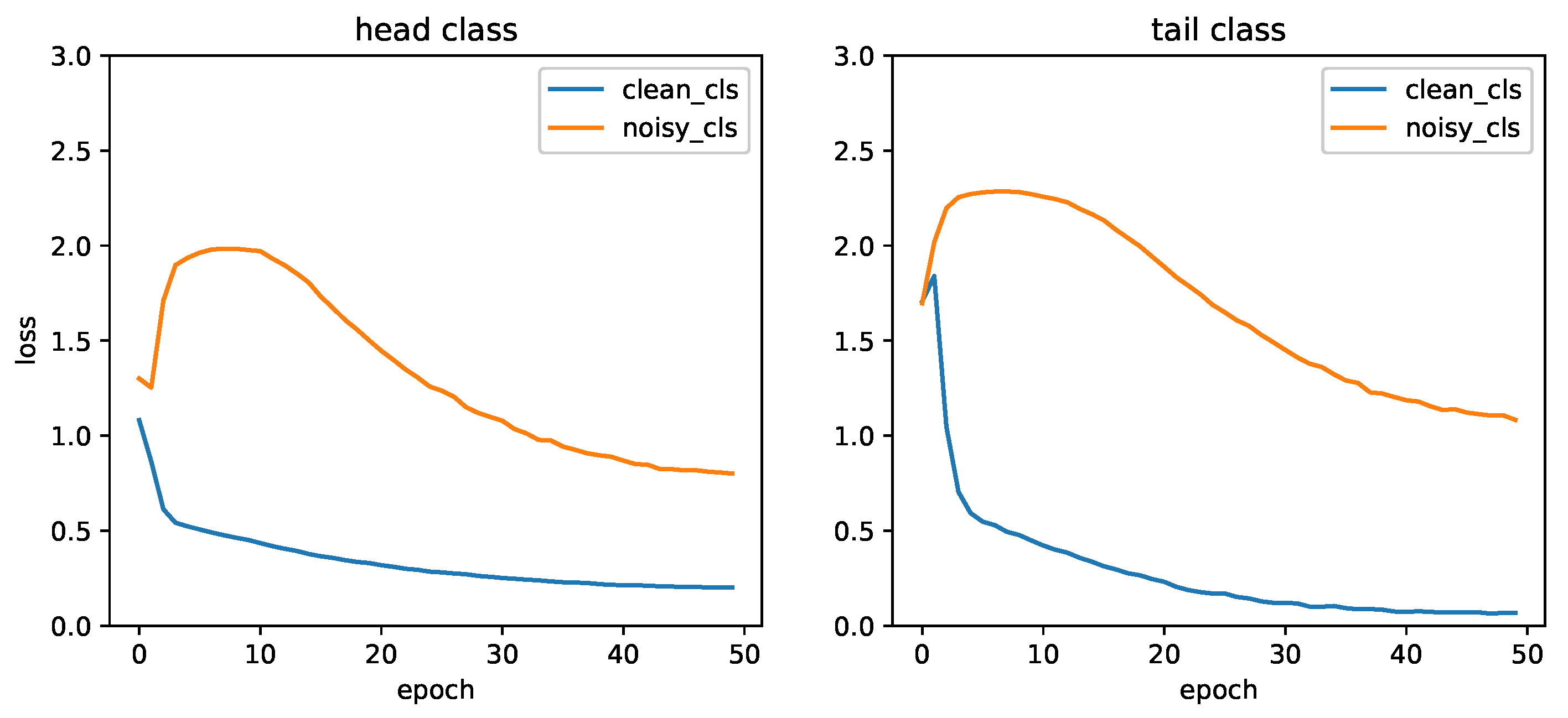To address the aforementioned challenges and drawing inspiration from the work of [14], we adopt a two-stage training strategy. In the first stage, we employ a pre-trained model to obtain multiple loss variation values for each epoch of all samples and fuse these values with attention features, which are semantic features extracted by multi-head self-attention layers, to enhance the discrimination among samples. 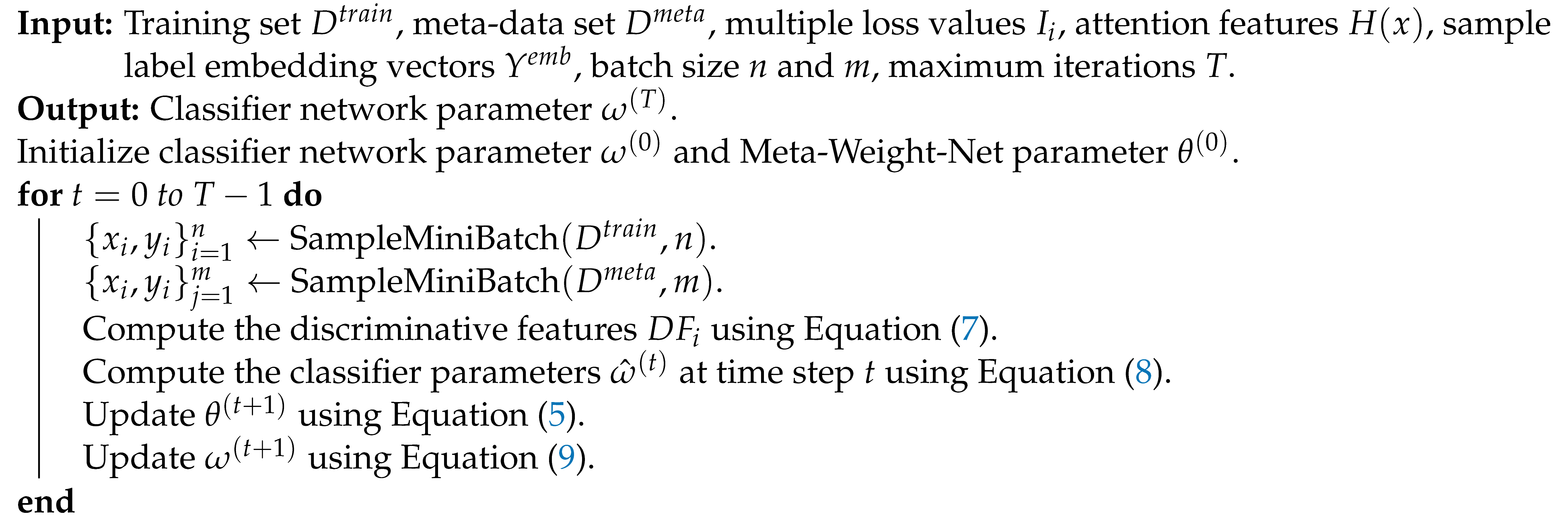We observe that the variation pattern of the pre-collected average training loss values (as illustrated in Figure 1) is similar to the findings of [14]. In the second stage, leveraging the high generalization capability of meta-learning, MLRNet calculates weights based on the fused sample features and analyzes the loss variation for each sample, assigning more reasonable weights and obtaining the final weighted loss values through a bi-level optimization problem with the classifier.

In summary, our contributions are as follows:

• We propose a Meta-Loss Reweighting Network (MLRNet) based on the concept of meta-learning with attention features, which performs well on complex biased situations.
• We embed the labels of samples, concatenate them with the features extracted by self-attention layers, and fuse it with pre-collected sample multi-loss variation values. This fused representation is referred to as the discriminative feature (or DF). Through MLRNet analysis of discriminative features, we identify the bias type of each sample and automatically assign appropriate weights to biased data.
• We conduct experiments on several English and Chinese benchmark datasets, including artificially generated and real-world biased datasets. The results demonstrate that our approach achieves better and more generalizable performance than prior works.

The structure of the paper is organized as follows: Section 2 discusses related work, Section 3 presents our proposed method, Section 4 demonstrates the experimental results and analysis, and Section 5 concludes the paper.

2. Related Work

2.1. Class Imbalance

Resampling the dataset is an effective measure to address class imbalance. Several methods include the SMOTE series, which involves over-sampling the minority class samples [15,16,17], under-sampling the majority class samples, and ensemble learning [18]. Another popular approach is data augmentation for tail class samples [19] using methods like synonym replacement, random insertion, random swapping, and random deletion. However, these methods may introduce new issues, such as overfitting with over-sampling and loss of valuable sample information with under-sampling. Additionally, these methods often require frequent parameter tuning to achieve better performance, resulting in higher average training iterations and expensive processing costs, particularly for large-scale datasets. Moreover, another prevalent choice is using sample reweighting methods, which involve two strategies. The first approach considers high loss-value samples to be more likely from the minority class and employs a monotonically increasing weighting function to force the model to learn from high-loss samples, such as AdaBoost [20] and focal loss [11]. The second approach introduces weighting functions based on the frequency of sample labels, such as the inverse of the class frequency [21] or the inverse square root [22]. Ref. [23] extended the traditional paradigm of imbalanced classification problems from discrete value domains to continuous value domains.

2.2. Corrupted Labels

To tackle label noise, refs. [5,8,24] assume the underlying causes of label noise and employ label correction processes to transform corrupted labels into cleaner ones. These methods require estimating a label corruption matrix, which is independent of the model training process. However, such estimations do not consider data-related noise, which is common in real-world label noise scenarios [25]. Ref. [26] expanded label correction by incorporating an additional meta-update process during normal training. They used a small amount of unbiased data to introduce meta-labels representing the reliability of each label. Through a meta-learning network, they dynamically adjusted the weights of each meta-label, enabling adaptive label noise correction during the training process. Another approach is reweighting the loss values of each sample, where samples with higher loss values are considered more likely to be noisy, and the model tends to focus on those high-confidence samples with clean labels. This is often achieved through methods like the SPL series [10].

2.3. Meta-Learning Combined with Reweighting

Meta-learning is a popular research direction in machine learning that allows models to rapidly adapt to new tasks with very few training data. Inspired by previous works [13,27,28], some automatic weighting methods using meta-learning have been proposed. They use a small amount of unbiased meta-data to automatically fit a more reasonable weighting function, which exhibits better generalization ability than manually adjusted hyperparameters [29] and demonstrates superior performance in data selection [30]. Typical meta-learning reweighting methods include MentorNet, L2RW, MW-Net, and CurveNet, which guide the model to assign weights to samples with the help of a small amount of unbiased data. These weights effectively act as hyperparameters for the classifier, which can be solved by solving a bi-level optimization problem between the classifier and the meta-network [31,32]. Specifically, MentorNet uses a bidirectional LSTM-based network to weight mini-batch samples in StudentNet, jointly optimizing deep CNNs for large-scale data. L2RW and MW-Net follow a similar structure, simultaneously learning the classifier and the weighting function. The classifier undergoes traditional gradient updates, while the weighting function is updated through meta-learning, alternating between the two. This function assigns weights to examples to alleviate overfitting caused by label corruption or class imbalance in the training data.

Furthermore, recently, a two-stage training strategy has been proposed [33,34,35] to improve the model’s classification performance on biased data. CurveNet [14] adopts a similar two-stage training strategy and discovers different changing trends in the loss curves of image samples with different types of biases.

Taking inspiration from the aforementioned works, we adopt a similar two-stage strategy, using multiple loss variation values. We improve the data flow between models by extracting attention features for each sample before obtaining the final classification result from the classifier’s output. These attention features, along with the sample’s label embedding and loss variation values, are fused to create what we call a sample discriminative feature. The classifier and meta-network learn from this discriminative feature during the training process, making them more sensitive to label-corrupted and class-imbalanced samples. This allows more reasonable weight allocation for biased training data that simultaneously contains noisy labels and imbalanced classes. As

Table 1. Performance comparisons on AG News with varying noise rates and imbalance factors.

Imbalance Ratio	10	20	50	100	200	1
Noise Rate	0					0	0.2	0.4
Bert-base	90.58	89.33	85.21	81.18	69.01	93.44	92.19	90.13
MW-Net	91.48	90.20	87.79	84.58	80.37	93.44	93.27	91.23
MLC	91.91	88.75	78.63	75.41	73.87	94.57	93.70	91.76
MLRNet(Ours)	92.15	89.95	90.07	88.47	83.22	94.21	94.10	92.38

The best results are highlighted in bold.

shows, our method achieves favorable performance in both high-class imbalance and high noise levels situations.

3. The Proposed Meta-Loss Reweighting Net Method

3.1. Optimization Objective in Meta-Learning

Following the work of [36], we perform model learning on two sets of data: a large set containing biased data and a small set of clean and unbiased data. Due to the high cost of expert labeling, the clean and unbiased dataset is much smaller than the biased dataset. Using the biased dataset as the entire training set is not optimal, since it contains a large amount of biased data. On the other hand, training solely on the clean dataset leads to severe overfitting due to the limited number of samples. To address this, we adopt the idea of meta-learning, where we use the small unbiased dataset as the meta-dataset to guide the parameter updates of both the classifier and the meta-network.

Let us represent the training set containing biased data as $D^{train}={\{x_i,y_i\}}_{i=1}^N$ and the meta-dataset as $D^{meta}={\{x_j,y_j\}}_{j=1}^M$, where N and M represent the sample sizes of the training set and the meta-dataset, respectively, and $N>>M$.

We use $X^{train}$ and $Y^{train}$ to denote all the samples and label vectors in the training set $D^{train}$, respectively. Similarly, $X^{meta}$ and $Y^{meta}$ represent all the samples and label vectors in the meta-dataset $D^{meta}$. The classifier is denoted by F, and its learnable parameters are represented as $\omega$. The regular parameters can be obtained by minimizing the following loss function:

$${\omega }^{*}=arg\underset{\omega }{min}\frac{1}{N}L\left(Y^{train},F\left(X^{train};\omega \right)\right)$$

(1)

Here, we use $L^{train}\left(\omega \right)$ as shorthand for $L(Y^{train},F(X^{train};\omega ))$. However, due to the presence of biased data, we need to assign weights to sample loss values to adjust the impact of biased data and improve the model’s robustness. We use $V(l;\theta )$ to represent the weight net, where $\theta$ represents its learnable parameters. Clearly, once $\theta$ is set to be optimal, we can obtain the optimal $w^{*}$ value, and Equation (1) can be written in the following weighted loss form:

$${\omega }^{*}=arg\underset{\omega }{min}\frac{1}{N}V\left(L^{train}\left(\omega \right);\theta \right)L^{train}\left(\omega \right)$$

(2)

The optimal $\theta$ can be obtained by minimizing the following loss function:

$${\theta }^{*}=arg\underset{\theta }{min}\frac{1}{M}L\left(Y^{meta},F\left(X^{meta};{\omega }^{*}\left(V\left(\theta \right)\right)\right)\right)$$

(3)

3.2. Bi-Level Optimization Parameter Update

As evident from Equations (2) and (3), it is apparent that the optimal $\theta$ cannot be directly determined because it requires the optimal $\omega$, and conversely, the optimal $\omega$ also depends on the optimal $\theta$ for its calculation. If we were to compute ${\omega }^{*}$, we would need to execute Equations (2) and (3) for each $\theta$, making the computations prohibitively expensive. The optimization of parameters for both the classifier and the weight net constitutes a bi-level optimization problem [13] that requires simultaneously optimizing the upper-level parameters (parameters of the weight net) and the lower-level parameters (classifier parameters). Therefore, on a mini-batch, we independently optimize the lower-level parameter $\omega$ using Equation (4) to approximate the optimal values. Subsequently, we optimize the upper-level parameter $\theta$ using Equation (5):

$${\widehat{\omega }}^{\left(t\right)}={\omega }^{\left(t\right)}-\alpha \frac{1}{n}V\left(L^{train}\left({\omega }^{\left(t\right)}\right);{\theta }^{\left(t\right)}\right)\frac{\partial }{\partial \omega }\left(L^{train}\left(\omega \right){|}_{{\omega }^{\left(t\right)}}\right)$$

(4)

$${\theta }^{\left(t+1\right)}={\theta }^{\left(t\right)}-\beta \frac{1}{m}\frac{\partial }{\partial \theta }\left(L^{meta}\left({\widehat{\omega }}^{\left(t\right)}\left(\theta \right)\right){|}_{{\theta }^{\left(t\right)}}\right)$$

(5)

Here, $\alpha$ and $\beta$ are the learning rates for $\omega$ and $\theta$, respectively. n and m represent the number of samples in a mini-batch from the training set and the meta-set, respectively. t denotes the current training epoch. After obtaining the optimal weight net parameters for the mini-batch, we can further update $\omega$ using Equation (6) to obtain the optimal classifier parameters:

$${\omega }^{\left(t+1\right)}={\omega }^{\left(t\right)}-\alpha \frac{1}{n}V\left(L^{train}\left({\omega }^{\left(t\right)}\right);{\theta }^{\left(t+1\right)}\right)\frac{\partial }{\partial \omega }\left(L^{train}\left(\omega \right){|}_{{\omega }^{\left(t\right)}}\right)$$

(6)

By iteratively performing these updates during training, we aim to find the optimal parameters for both classifier and weight net, effectively addressing the issue of biased data and improving the model’s performance on biased training data.

3.3. Discriminative Features

Inspired by previous works, we also adopt a similar two-stage training strategy. In the first stage, we collect the loss values of each sample for every epoch using the loss function $L(Y^{train},F(X^{train};\omega ))$. These loss variation values are represented as $L_i=[L_i^0,L_i^1,\cdots L_i^t,\cdots L_i^T]$, where T represents the total number of training epochs $(0\le t\le T)$. We then normalize the multiple loss values for each sample by subtracting the average loss of the corresponding class, which highlights the difference between clean and biased samples. We denote the normalized loss variation values of a sample as $I_i$.

In the field of NLP (Natural Language Processing), pre-trained models have rapidly developed and achieved impressive results on downstream tasks such as classification [37,38,39]. We use a pre-trained model as the classifier and extract the vector before the model’s output as the feature representation $h\left(x_i\right)$ for each sample. It is important to note that before using this feature vector, we apply a stop-gradient operation; this is because we only use $H\left(x\right)$ as the sample’s feature during forward propagation and do not want gradients to flow back to the classifier during backward propagation. Additionally, we embed the sample’s label to obtain the label-embedding vector $Y^{emb}\left(y_i\right)$. This label-embedding method is commonly used in the domain of biased data [26,40]. We concatenate the sample feature $H\left(x\right)$ with $Y^{emb}$, aiming to preserve the original attributes that can represent the sample’s information. The concatenated sample features are fed as inputs to the subsequent linear layer with a tahh activation function. On the other hand, we pass $I_i$ through a fully connected layer with a Tanh activation function. By summing the input of this layer and the concatenated sample features, we obtain a vector that fully incorporates the sample’s semantic information and has high discriminability among samples. We refer to this vector as the discriminative feature ${DF}_i$:

$$DF(H\left(x\right),Y^{emb},I_i)=concat(h(x_i,Y^{emb}\left(y_i\right))+Dense\left(I_i\right)$$

(7)

3.4. The Meta-Loss Reweighting Network (MLRNet) with Discriminative Features (DF)

MLRNet takes the discriminative features as inputs. Therefore, the parameter update Equations (4) and (6) of the model can be rewritten as follows:

$${\widehat{\omega }}^{\left(t\right)}={\omega }^{\left(t\right)}-\alpha \frac{1}{n}V\left(DF\left(H\left(x\right),Y^{emb},I_i\right);{\theta }^{\left(t\right)}\right)\frac{\partial }{\partial \omega }\left(L^{train}\left(\omega \right){|}_{{\omega }^{\left(t\right)}}\right)$$

(8)

$${\omega }^{\left(t+1\right)}={\omega }^{\left(t\right)}-\alpha \frac{1}{n}V\left(DF\left(H\left(x\right),Y^{emb},I_i\right);{\theta }^{\left(t+1\right)}\right)\frac{\partial }{\partial \omega }\left(L^{train}\left(\omega \right){|}_{{\omega }^{\left(t\right)}}\right)$$

(9)

To summarize, in the second stage, guided by a small amount of unbiased data, the classifier and the meta-net are jointly optimized. After training the classifier for a certain number of iterations, we use the meta-model to update the classifier’s parameters to obtain suboptimal parameters based on Equation (8). Next, we update and obtain the optimal upper-level parameters from the meta-set by using Equation (5). Finally, using Equation (9) on the biased dataset, we obtain the optimal lower-level parameters, completing the bi-level optimization for both the main model and the weight net. The entire training process is illustrated in Figure 2, and the parameter update algorithms for both the classifier and the meta-model are detailed in Algorithm 1. The introduction of discriminative features makes the model more sensitive to the types of data bias, thereby allocating more reasonable weights to biased training data that simultaneously contain corrupted labels and imbalanced classes.

Algorithm 1: The MLRNet Training Algorithm

4. Experiments

To evaluate the proposed algorithm’s performance, we conduct experiments on benchmark datasets in both English and Chinese. These datasets comprise both synthetic and real-world biased datasets, allowing us to assess the algorithm’s generalizability in various scenarios. We compared the algorithm against existing methods under different imbalance factors and noise levels to gauge its effectiveness.

4.1. Datasets

AG News: This is a large-scale multi-class text classification benchmark dataset containing 496,835 news articles from over 2000 different news sources. Following the work of [41], we focused on the four classes with the most samples and used the article titles along with their corresponding descriptions. In the training set, each class has 30,000 samples, while in the test set, each class has 1900 samples. For fair comparison (MLC), we randomly selected 100 samples from each class to form a clean and unbiased meta-dataset.

CLUE: A Chinese language understanding evaluation benchmark [42]. For our experiments, we selected two datasets from the classification tasks, TNEWS and IFLYTEK. TNEWS is a dataset that contains 73,360 news headlines for short text classification. It covers 15 categories, and the training, validation, and test sets consist of 53.3 k, 10 k, and 10 k samples, respectively. IFLYTEK is a dataset that includes 17,332 app descriptions for long text classification. It has 119 categories, and the dataset is split into 12.1 k, 2.6 k, and 2.6 k samples for training, validation, and test sets, respectively.

Real-World Noise: DataCLUE is a benchmark that replaces the traditional model-centric approach with a data-centric approach for Chinese text classification [43]. We used the CIC Electronic Commerce 118-classification dataset from DataCLUE because it contains a high proportion of mislabeled data and a large number of label categories with certain imbalances in the label distribution. This dataset is used as a real-world biased dataset. The data are split into 10,000 samples for training, 2000 samples for validation, and 2000 samples for the test set. Notably, more than 1/3 of the training set and more than 1/5 of the validation set have mislabeled data, while the test set has ground-truth labels with an accuracy exceeding 95%.

It is worth noting that AG News is a large-scale dataset without biased data, but the other three datasets, THNEWS, IFLYTEK, CIC, are all naturally biased and have smaller scales than AG NEWS. Therefore, we additionally set the bias for the AG News dataset and experimentally verified the performance of our method on the large-scale dataset under different bias combinations. Thus, we constructed a biased training set for the AG news dataset using the two types of bias settings mentioned in Section 4.2 and conducted experiments on it.

4.2. Bias Setup

Class Imbalance: To create a class-imbalanced dataset, we gradually reduced the number of samples for each class using an exponential function $n=n_i{\mu }^i$, where i is the index of the class, $n_i$ is the original number of samples for each class, and $\mu \in (0,1)$. The imbalance level of the dataset is defined by an imbalance factor, which is the ratio of the number of training samples in the largest class to the number of training samples in the smallest class. For example, when the imbalance factor is 100, assuming the class with the most samples has 1200 samples, the class with the fewest samples contains only 12 samples.

Label Noise: We used two commonly used methods to introduce label noise: uniform noise and flipping noise. Both methods change the label of a sample to another label with a probability of noise level p.

UNIFORM: Suppose the dataset contains C classes. In the uniform noise setting, the sample’s label is preserved with a probability of $1-p$. The label is randomly corrupted to other labels with equal probability $\frac{p}{C}$ for each class. The UNIFORM noise matrix is defined as follows: for each element $a_{ij}$ in the matrix, it represents the probability that the label with index i is corrupted to the label with index j.

$$corruptedmatrix=\left[\begin{array}{ccccc}1-p+\frac{p}{C}& \frac{p}{C}& \dots & \dots & \frac{p}{C}\\ ⋮& ⋮& ⋮& ⋮& ⋮\\ \frac{p}{C}& \dots & 1-p+\frac{p}{C}& \dots & \frac{p}{C}\\ ⋮& ⋮& ⋮& ⋮& ⋮\\ \frac{p}{C}& \dots & \dots & \frac{p}{C}& 1-p+\frac{p}{C}\end{array}\right]$$

FLIP: In the FLIP noise setting, we also assume a dataset with C classes. Similar to the uniform noise, the label is preserved with a probability of $1-p$. However, with a probability of p, the label is corrupted to one of the remaining $C-1$ classes specified randomly. For example, for the label with index 0, the FLIP noise matrix may look like $\left[\begin{array}{ccccc}1-p& 0& p& \dots & 0\end{array}\right]$. Due to its randomness, the complete FLIP noise matrix is not provided here.

4.3. Hyperparameter Configuration for the MLRNet

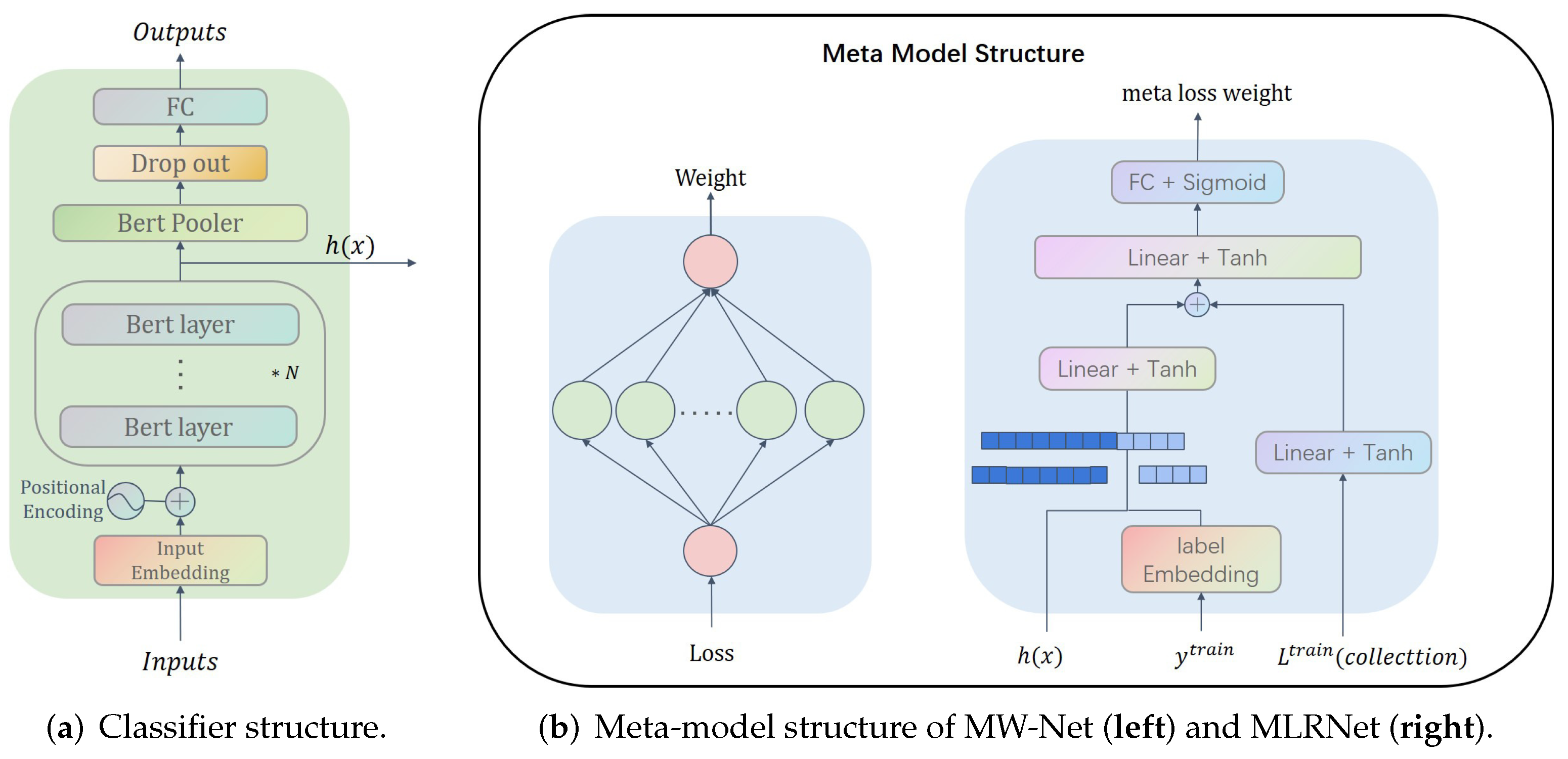
We maintained a consistent configuration similar to MLC by setting the dimensionality of the attention features extracted by the classifier to 768. Simultaneously, we established the size of the label embedding layer as $(C,128)$, where C represents the number of classes in the dataset. We then processed $I_i$ through three layers of Tanh activation functions, resulting in an output dimensionality equivalent to that of the discriminative features.

Given that attention features are concatenated with label embedding vectors, the concatenated representation subsequently passes through two layers of Tanh activation functions. The input dimensionality here is the sum of the feature dimension and the label embedding dimension, while the output dimension matches that of the discriminative features. Summation is performed to obtain the discriminative features $D{F}_i$.

Following this, a three-layer feedforward network with Tanh activation functions is employed, which is followed by a final layer with a sigmoid activation function. This ensures that the computed weights fall within the [0, 1] range. The structural visualization of this model can be referenced in Figure 3.

4.4. Implement Details

AG News: We constructed datasets with different bias proportions by artificially reducing the number of samples in each category and corrupting the labels with noise using the noise matrices. The model was trained for 10 epochs on an NVIDIA RTX A5000 GPU. We utilized the pre-trained BERT-base-uncased model as the backbone network with a batch size of 30. The learning rate for the classifier was set to 1 × ${10}^{-5}$ and we set the random seed to 1 to ensure the results are replicable in multiple runs.

Other datasets: For fairness, for Chinese datasets such as IFLYTEK, TNEWS and CIC, we used different models as classifiers and conducted different experiments on each dataset. Following previous work [42,43], we utilized the pre-trained RoBERTa-l3 model as the backbone network with a batch size of 16. This model was trained for 6 epochs on an NVIDIA RTX A5000 GPU. The learning rate for the classifier was set to 2 × ${10}^{-5}$, and we set the random seed to 42 to ensure the results are replicable in multiple runs.

For the CIC dataset, [43] used Macro-F1 as the primary evaluation metric. In this paper, we use accuracy as the evaluation metric for the experimental results of all English and Chinese datasets, which is the percentage of the number of correctly predicted samples divided by the total number of samples by the model. To maintain consistency for comparison, we adopted the same hyperparameter settings as [43].

It is worth noting that in today’s prevalent pre-training models, such as BERT, the Post-Norm structure can lead to the problem of gradient vanishing during backpropagation, especially in deeper layers [44,45]. However, this seems to align with the original design intention of pre-trained models, aiming to preserve the effectiveness of pre-trained layers as much as possible. To address this, we used the Adam optimizer for training, and its warm-up mechanism allowed the model to start with a smaller learning rate to familiarize itself with the overall data distribution. For the same dataset, each model was trained with the same number of warm-up steps and epochs.

4.5. Comparison Method

Due to factors such as scale, manual construction, and language differences, AG news is a large-scale English dataset without biased data, while the other datasets are small-scale biased Chinese datasets. Therefore, we use the state-of-the-art comparison methods of the current dataset for comparison.

For the AG News dataset, we conducted experiments with different setting of bias, which included cases of extreme class imbalance and extreme label noise. For example, in Table 1, an imbalance factor of 200 means that the class with the highest number of samples has 200 times the number of samples compared to the class with the lowest number. The main comparison was made with two SOTA methods: [36] used meta-learning for sample reweighting (referred to as MW-Net), and [26] used meta-learning for label correction (referred to as MLC). The label correction model represented by MLC performs poorly on high class imbalance, so we conducted additional experiments under complete label noise settings. The values in

Table 2. Mean accuracies on AG News under two noise types and 10 noise levels.

Method	Bert-Base	MW-Net	GLC	MLC	MLRNet (Ours)
Accuracy(%)	74.65	75.91	83.88	85.27	85.41

The best results are highlighted in bold.

represent the average accuracy of 10 noise levels for each of the two bias construction methods (UNIFORM and FLIP); for example, UNIFORM noise level 0.2 and FLIP noise level 0.8 indicates whether to use UNIFORM or FLIP to construct noise, and 20% or 80% of sample labels are replaced with noisy labels. GLC [5] and MLC are the best models for handling label noise in weakly supervised label correction models.

Result on the Chinese Benchmark Datasets

We further evaluated our approach on the Chinese benchmark datasets, and the results are presented in

Table 3. Performance comparisons on Chinese benchmark datasets.

Method	RoBERTa-l3	Bert-wwm-ext	RoBERTa-wwm-ext	MW-Net	MLRNet (Ours)
THNEWS	55.43	56.84	56.94	57.03	59.30
IFLYTEK	58.67	59.43	60.31	59.74	61.45
CIC	84.45	84.90	84.70	84.69	85.35

The best results are highlighted in bold.

. The experimental outcomes affirm that our methodology also yields commendable results on the Chinese dataset, thus underscoring its versatility and efficacy across diverse tasks.

For other Chinese benchmark datasets, we also follow the work of previous researchers [42,43] and use their baseline for comparison, such as RoBERTa-l3 [39], Bert-wwm-ext [46] and RoBERTa-wwm-ext [46]. BERT-WWM is the first pre-training scheme designed for the Chinese language, which uses a whole word mask (WWM) strategy based on Chinese words. Compared to individual Chinese character-based masks, word-based masks enable the model to learn more semantic information. BERT-wwm-ext adopts the same model structure as BERT-wwm, consisting of 12 layers of bert layers. In fact, it is able to increase the training dataset and training steps to improve the effect. RoBERTa changed the pre-training strategy and removed the Next Sentence Prediction (NSP) task; it is trained with dynamic masking. Thus, RoBERTa-wwm-ext is a Roberta model that uses the WWM strategy and increases the training dataset and training steps. RoBERTa-l3 is a RoBERTa-wwm-ext model but with three Bert layers.

In addition, MW-Net [36], as the state-of-the-art meta-learning reweighting method with strong universality and robustness, runs through all comparison methods.

4.6. Experiments Results and Analysis

4.6.1. Results on the English Benchmark Dataset

We conducted a comparative analysis of model performance on the AG News dataset across various imbalance factors and noise levels. The experimental results presented in Table 1 demonstrate that when utilizing Bert-base as the backbone network, MLRNet consistently exhibits robust performance across most settings. It is noteworthy that in this context, the noise labels were generated using the UNIFORM method. Importantly, when the noise level is set to 0, the task effectively transforms into a single-class imbalance problem. Similarly, when the imbalance factor is set to 1, it becomes a single-class label corruption problem. The observations reveal that concerning class imbalance, as the imbalance factor gradually increases, MWN outperforms other models, while MLC, functioning as a label correction model, demonstrates relatively weaker performance. Conversely, in terms of label corruption, MLC outperforms MW-Net. Notably, MLRNet consistently achieves favorable results particularly in scenarios characterized by high class imbalance and noise levels.

Furthermore, we investigated two methods for constructing label noise. The values in Table 2 represent the average results obtained from 20 (2 × 10) different settings with each method (UNIFORM and FLIP) comprising 10 noise levels. Each configuration was run five times to ensure robustness. MLRNet demonstrated robust performance even under extreme label noise conditions.

4.6.2. Ablation Study and Analysis

In order to explore the versatility of MLRNet across different backbone networks, we substituted the backbone network with Bert-base-3l, which comprises only three layers of attention layers, and conducted further experiments on the AG News dataset. We configured imbalance factors for bias data types as [1, 10, 20], employed label noise of the UNIFORM type, and varied noise levels within the range [0.0, 0.2, 0.4, 0.6]. Building upon these settings, we conducted a detailed investigation into our methodology to ascertain its adaptability to diverse bias scenarios. The outcomes of these experiments are presented in

Table 4. Acuracy of our model with Bert-base-l3 on AG News.

Imbalance-Ratio	10			20
Noise-Rate	0.2	0.4	0.6	0.2	0.4	0.6
Bert-base	89.41	88.77	87.43	87.53	86.18	84.88
MW-Net	90.26	89.62	88.36	88.65	88.12	86.71
MLRNet (Ours)	91.23	90.18	88.82	89.77	89.71	88.39

The best results are highlighted in bold.

.

Effects of the number of Meta-Samples. Given the inherent errors in data collection and the substantial cost associated with expertly annotating unbiased datasets, we systematically varied the quantity of meta-samples during training to further validate the robustness of our method. As delineated in

Table 5. Accuracy under varying numbers of meta-samples on AG News.

Method	Bert-Base	MLRNet (Ours)						MW-Net
Num	-	10	20	50	100	200	500	200
Accuracy (%)	86.18	87.11	87.17	87.25	88.68	89.71	88.80	88.12

The best results are highlighted in bold.

, our approach demonstrates noteworthy performance, even when the number of meta-samples per class is as low as 10, resulting in a notable improvement of 1.24% (imbalance factor set at 20, noise level at 0.4, and DF feature dimensionality at 128). Interestingly, as the quantity of meta-samples per class gradually increases, this improvement becomes even more pronounced. It is worth noting, however, that when the number of meta-samples per class reaches 500, there is a decline in accuracy, as illustrated in Figure 4. We attribute this phenomenon to the fact that an excessively large meta-dataset exacerbates the bias within the training set, ultimately leading to a decrease in accuracy. Hence, we emphasize the importance of an appropriately sized meta-dataset in achieving optimal results.

Effects of discriminative feature dimensionality. Given that the dimensionality of discriminative features directly impacts the computational workload and training speed of the meta-model, we conducted experiments by adjusting the dimensionality of discriminative feature embeddings. The results are presented in

Table 6. Accuracy under varying dimensionality of DF on AG News.

DF Dimensionality	32	64	128	256	768
Accuracy (%)	88.50	88.36	89.71	90.04	90.35

The best results are highlighted in bold.

(imbalance factor set at 20, noise level at 0.4, and 200 meta-samples per class). Concurrently, as evident from Figure 5, it is apparent that with an increase in DF dimensionality, the average accuracy steadily improves, underscoring the pivotal role of discriminative features. However, the escalation in DF dimensionality also leads to a substantial increase in model parameters, resulting in extended training times and heightened training costs. Consequently, taking into account factors both performance and training time, we opted for a DF dimensionality of 128.

5. Conclusions and Future Work

This paper introduces a novel MLRNet meta-module capable of handling highly biased datasets, which can be applied to various tasks to enhance their performance. It leverages the evolving trends in sample loss values to provide valuable insights for distinguishing different biased samples. Within MLRNet, we propose a meta-loss reweighting network structure that incorporates attention features. We introduce the concept of discriminative features, employing a two-stage training strategy to pre-collect multiple loss variation values for each sample and fuse them with sample feature vectors extracted through self-attention layers. This enhances the discriminative capability of biased data samples. Leveraging meta-learning principles, we train the entire model to assign more reasonable weights to biased samples. Our experimental results on publicly available datasets in both English and Chinese demonstrate the practicality of our approach, particularly in scenarios where dataset is highly biased.

It is important to note that our experiments have been primarily conducted in the domain of text classification. Our future work will explore research in the field of image recognition. However, the meta-learning ideas and dynamic sample weighting methods provided by MLRNet may not be limited to text and image classification. Its architecture and principles may be applicable to other fields, such as speech recognition, medical image analysis, and financial data mining, especially when there is significant bias in the dataset. In the future, it may be used to improve the robustness of models in real-world data and help develop models that are more adaptable to real-world diversity. With data bias becoming a common problem in machine learning, the introduction of MLRNet marks a beneficial exploration of this challenge. Future research may further explore model optimization methods under different types of biases as well as their applications in a wider range of fields.

References

1. Ren, M.; Zeng, W.; Yang, B.; Urtasun, R. Learning to reweight examples for robust deep learning. In Proceedings of the International Conference on Machine Learning, Stockholm, Sweden, 10–15 July 2018; pp. 4334–4343. [Google Scholar]
2. Gong, R.; Qin, X.; Ran, W. Prompt-Based Graph Convolution Adversarial Meta-Learning for Few-Shot Text Classification. Appl. Sci. 2023, 13, 9093. [Google Scholar] [CrossRef]
3. He, H.; Garcia, E.A. Learning from imbalanced data. IEEE Trans. Knowl. Data Eng. 2009, 21, 1263–1284. [Google Scholar]
4. Zhang, C.; Bengio, S.; Hardt, M.; Recht, B.; Vinyals, O. Understanding deep learning (still) requires rethinking generalization. Commun. ACM 2021, 64, 107–115. [Google Scholar] [CrossRef]
5. Hendrycks, D.; Mazeika, M.; Wilson, D.; Gimpel, K. Using Trusted Data to Train Deep Networks on Labels Corrupted by Severe Noise. arXiv 2018, arXiv:1802.05300. [Google Scholar]
6. Reed, S.; Lee, H.; Anguelov, D.; Szegedy, C.; Erhan, D.; Rabinovich, A. Training deep neural networks on noisy labels with bootstrapping. arXiv 2014, arXiv:1412.6596. [Google Scholar]
7. Kaya, M. Feature fusion-based ensemble CNN learning optimization for automated detection of pediatric pneumonia. Biomed. Signal Process. Control. 2024, 87, 105472. [Google Scholar] [CrossRef]
8. Jiang, L.; Zhou, Z.; Leung, T.; Li, L.J.; Li, F.F. Mentornet: Learning data-driven curriculum for very deep neural networks on corrupted labels. In Proceedings of the ICML 2018, Stockholm, Sweden, 10–15 July 2018. [Google Scholar]
9. Neshir, G.; Rauber, A.; Atnafu, S. Meta-Learner for Amharic Sentiment Classification. Appl. Sci. 2021, 11, 8489. [Google Scholar] [CrossRef]
10. Kumar, M.P.; Packer, B.; Koller, D. Self-Paced Learning for Latent Variable Models. In Proceedings of the International Conference on Neural Information Processing Systems, Vancouver, BC, Canada, 6–9 December 2010. [Google Scholar]
11. Lin, T.Y.; Goyal, P.; Girshick, R.; He, K.; Dollár, P. Focal Loss for Dense Object Detection. IEEE Trans. Pattern Anal. Mach. Intell. 2017, 42, 318–327. [Google Scholar]
12. Wang, X.; Du, Y.; Chen, D.; Li, X.; Chen, X.; Fan, Y.; Xie, C.; Li, Y.; Liu, J. Improving Domain-Generalized Few-Shot Text Classification with Multi-Level Distributional Signatures. Appl. Sci. 2023, 13, 1202. [Google Scholar] [CrossRef]
13. Finn, C.; Abbeel, P.; Levine, S. Model-agnostic meta-learning for fast adaptation of deep networks. In Proceedings of the International Conference on Machine Learning, Sydney, NSW, Australia, 6–11 August 2017; pp. 1126–1135. [Google Scholar]
14. Jiang, S.; Li, J.; Wang, Y.; Huang, B.; Zhang, Z.; Xu, T. Delving into Sample Loss Curve to Embrace Noisy and Imbalanced Data. Proc. AAAI Conf. Artif. Intell. 2022, 36, 7024–7032. [Google Scholar] [CrossRef]
15. Chawla, N.V.; Bowyer, K.W.; Hall, L.O.; Kegelmeyer, W.P. SMOTE: Synthetic Minority Over-sampling Technique. J. Artif. Intell. Res. 2002, 16, 321–357. [Google Scholar] [CrossRef]
16. Han, H.; Wang, W.Y.; Mao, B.H. Borderline-SMOTE: A New Over-Sampling Method in Imbalanced Data Sets Learning; Lecture Notes in Computer Science; Springer: Berlin/Heidelberg, Germany, 2005. [Google Scholar]
17. Georgios, D.; Fernando, B.; Felix, L. Improving imbalanced learning through a heuristic oversampling method based on k-means and SMOTE. Inf. Ences 2018, 465, 1–20. [Google Scholar]
18. Liu, X.Y.; Wu, J.; Zhou, Z.H. Exploratory Undersampling for Class-Imbalance Learning. In Proceedings of the Systems, Man and Cybernetics, San Antonio, TX, USA, 11–14 October 2009. [Google Scholar]
19. Wei, J.; Zou, K. EDA: Easy Data Augmentation Techniques for Boosting Performance on Text Classification Tasks. arXiv 2019, arXiv:1901.11196. [Google Scholar]
20. Freund, Y.; Schapire, R.E. A decision-theoretic generalization of on-line learning and an application to boosting. J. Comput. Syst. Sci. 1997, 55, 119–139. [Google Scholar] [CrossRef]
21. Wang, Y.; Ramanan, D.; Hebert, M.H. Learning to model the tail. In Proceedings of the Neural Information Processing Systems, Long Beach, CA, USA, 4–9 December 2017. [Google Scholar]
22. Mahajan, D.; Girshick, R.; Ramanathan, V.; He, K.; Paluri, M.; Li, Y.; Bharambe, A.; Van Der Maaten, L. Exploring the limits of weakly supervised pretraining. In Proceedings of the European Conference on Computer Vision (ECCV), Munich, Germany, 8–14 September 2018; pp. 181–196. [Google Scholar]
23. Yang, Y.; Zha, K.; Chen, Y.; Wang, H.; Katabi, D. Delving into deep imbalanced regression. In Proceedings of the International Conference on Machine Learning, Online, 18–24 July 2021; pp. 11842–11851. [Google Scholar]
24. Yao, Y.; Liu, T.; Han, B.; Gong, M.; Deng, J.; Niu, G.; Sugiyama, M. Dual t: Reducing estimation error for transition matrix in label-noise learning. Adv. Neural Inf. Process. Syst. 2020, 33, 7260–7271. [Google Scholar]
25. Xia, X.; Liu, T.; Han, B.; Wang, N.; Gong, M.; Liu, H.; Niu, G.; Tao, D.; Sugiyama, M. Part-dependent label noise: Towards instance-dependent label noise. Adv. Neural Inf. Process. Syst. 2020, 33, 7597–7610. [Google Scholar]
26. Zheng, G.; Awadallah, A.H.; Dumais, S. Meta Label Correction for Noisy Label Learning. Proc. AAAI Conf. Artif. Intell. 2021, 35, 11053–11061. [Google Scholar] [CrossRef]
27. Shu, J.; Xu, Z.; Meng, D. Small sample learning in big data era. arXiv 2018, arXiv:1808.04572. [Google Scholar]
28. Antoniou, A.; Edwards, H.; Storkey, A. How to train your MAML. arXiv 2018, arXiv:1810.09502. [Google Scholar]
29. Hospedales, T.; Antoniou, A.; Micaelli, P.; Storkey, A. Meta-learning in neural networks: A survey. IEEE Trans. Pattern Anal. Mach. Intell. 2021, 44, 5149–5169. [Google Scholar] [CrossRef]
30. Lee, H.y.; Li, S.W.; Vu, N.T. Meta learning for natural language processing: A survey. arXiv 2022, arXiv:2205.01500. [Google Scholar]
31. Franceschi, L.; Frasconi, P.; Salzo, S.; Grazzi, R.; Pontil, M. Bilevel programming for hyperparameter optimization and meta-learning. In Proceedings of the International Conference on Machine Learning, Stockhom, Sweden, 10–15 July 2018; pp. 1568–1577. [Google Scholar]
32. Sinha, A.; Shaikh, V. Solving bilevel optimization problems using kriging approximations. IEEE Trans. Cybern. 2021, 52, 10639–10654. [Google Scholar] [CrossRef] [PubMed]
33. Svoboda, J.; Anoosheh, A.; Osendorfer, C.; Masci, J. Two-stage peer-regularized feature recombination for arbitrary image style transfer. In Proceedings of the IEEE/CVF Conference on Computer Vision and Pattern Recognition, Seattle, WA, USA, 13–19 June 2020; pp. 13816–13825. [Google Scholar]
34. Zhao, Z.; Tang, P.; Zhao, L.; Zhang, Z. Few-shot object detection of remote sensing images via two-stage fine-tuning. IEEE Geosci. Remote Sens. Lett. 2021, 19, 1–5. [Google Scholar] [CrossRef]
35. Valizadeh Aslani, T.; Shi, Y.; Wang, J.; Ren, P.; Zhang, Y.; Hu, M.; Zhao, L.; Liang, H. Two-stage fine-tuning: A novel strategy for learning class-imbalanced data. arXiv 2022, arXiv:2207.10858. [Google Scholar]
36. Shu, J.; Xie, Q.; Yi, L.; Zhao, Q.; Zhou, S.; Xu, Z.; Meng, D. Meta-weight-net: Learning an explicit mapping for sample weighting. arXiv 2019, arXiv:1902.07379. [Google Scholar]
37. Vaswani, A.; Shazeer, N.; Parmar, N.; Uszkoreit, J.; Jones, L.; Gomez, A.N.; Kaiser, L.; Polosukhin, I. Attention is all you need. arXiv 2017, arXiv:1706.03762. [Google Scholar]
38. Devlin, J.; Chang, M.W.; Lee, K.; Toutanova, K. Bert: Pre-training of deep bidirectional transformers for language understanding. arXiv 2018, arXiv:1810.04805. [Google Scholar]
39. Liu, Y.; Ott, M.; Goyal, N.; Du, J.; Joshi, M.; Chen, D.; Levy, O.; Lewis, M.; Zettlemoyer, L.; Stoyanov, V. Roberta: A robustly optimized bert pretraining approach. arXiv 2019, arXiv:1907.11692. [Google Scholar]
40. Cao, K.; Chen, Y.; Lu, J.; Arechiga, N.; Gaidon, A.; Ma, T. Heteroskedastic and Imbalanced Deep Learning with Adaptive Regularization. In Proceedings of the International Conference on Learning Representations, Virtual Event, Austria, 3–7 May 2021. [Google Scholar]
41. Zhang, X.; Zhao, J.; LeCun, Y. Character-level convolutional networks for text classification. arXiv 2015, arXiv:1509.01626. [Google Scholar]
42. Xu, L.; Hu, H.; Zhang, X.; Li, L.; Cao, C.; Li, Y.; Xu, Y.; Sun, K.; Yu, D.; Yu, C. CLUE: A Chinese language understanding evaluation benchmark. arXiv 2020, arXiv:2004.05986. [Google Scholar]
43. Xu, L.; Liu, J.; Pan, X.; Lu, X.; Hou, X. Dataclue: A benchmark suite for data-centric nlp. arXiv 2021, arXiv:2111.08647. [Google Scholar]
44. Xiong, R.; Yang, Y.; He, D.; Zheng, K.; Zheng, S.; Xing, C.; Zhang, H.; Lan, Y.; Wang, L.; Liu, T. On layer normalization in the transformer architecture. In Proceedings of the International Conference on Machine Learning, Honolulu, HI, USA, 23–29 July 2020; pp. 10524–10533. [Google Scholar]
45. He, R.; Ravula, A.; Kanagal, B.; Ainslie, J. RealFormer: Transformer Likes Residual Attention. In Proceedings of the Findings of the Association for Computational Linguistics: ACL-IJCNLP 2021, Online Event, 1–6 August 2021. [Google Scholar]
46. Cui, Y.; Che, W.; Liu, T.; Qin, B.; Yang, Z. Pre-training with whole word masking for chinese bert. IEEE/ACM Trans. Audio Speech, Lang. Process. 2021, 29, 3504–3514. [Google Scholar] [CrossRef]
Figure 1. The variation in average training loss for biased samples in the AG News. In the figure, it is evident that different types of biased samples exhibit distinct trends in their loss value variations (with an imbalance factor of 20 and noise label level of 0.4). Firstly, concerning the class imbalance issue, head class samples consistently display lower loss values compared to tail class samples. Secondly, for samples with noisy labels, their loss values are higher than those with undistorted labels. For head class samples, the loss values for clean label samples steadily decrease, while the loss values for samples with noisy labels initially decrease and then sharply increase before slowly decreasing again. Conversely, for tail class samples, the loss values for clean label samples initially experience an increase, which is followed by a significant decrease. In contrast, the loss values for samples with noisy labels first increase and then decrease.
Applsci 14 00164 g001
Figure 2. The training process of MLRNet. In the depicted diagram, the green-colored blocks represent the backbone network, serving as the classifier for the entire model. The blue-colored blocks represent the meta-model, MLRNet, with its network structure outlined at Figure 3. Within the black-bordered area in the diagram, we illustrate the process of optimizing and updating the meta-network parameters. The arrows in the diagram denote the flow of data, although, due to the complexity of the diagram, the three inputs to MLRNet are not explicitly depicted.
Applsci 14 00164 g002
Figure 3. The structure of classifier and meta-net. (a) illustrates the network architecture of the classifier (Bert-base), where N represents the number of layers in the Bert attention layers. (b) depicts the meta-net structures of MW-Net and MLRNet, respectively.
Applsci 14 00164 g003
Figure 4. Impact of meta-samples per-class.
Applsci 14 00164 g004
Figure 5. Impact of DF dimensionality.
Applsci 14 00164 g005