Nonlinear Tank-Level Control Using Dahlin Algorithm Design and PID Control

Abstract

Liquid-level control in tanks is widely used in various industrial sectors. Due to problems arising from the case that the liquid level is above or below the recommended, the process of its control is of great significance. The proportional integral differential (PID) controller is one of the most widely used controllers in applications that require accuracy and optimal automatic control. In this paper, single and coupled ship fuel tank systems are discussed. In addition, mathematical models and their linearization using two different approaches are presented. The two control approaches are used to maintain the specified liquid level in tanks. The first is based on the design of standard PID controllers, with the application of the Ziegler–Nichols, Takahashi tuning, and Auto-tuning methods. The second approach, proposed by the authors, is based on the application of the Dahlin algorithm. The simple modification of the Dahlin controller, which can avoid the “ringing” of the control signal, is suggested in the paper. Moreover, the lower limit of the decrease in the desired time constant, which ensures the desired behavior of the system, is determined. The comparisons provided for different performance indexes show the advantages of the modified Dahlin algorithm approach compared to the standard PID controllers. Furthermore, the comparison with the literature-known approaches is realized.

1. Introduction

The liquid-level control process is one of the primary issues in various industries, such as pharmaceutical, biochemical, nuclear, marine, etc. Usually, all analyses start with a single tank (ST) system [1,2,3,4], followed by a coupled tank (CT) system. In CT systems, liquids are generally pumped into tanks for further operations. Different types of CT systems described in literature depend on the number of liquid inlets and outlets [5,6,7].

Industrial processes utilize storage tanks of different geometries. Cylindrical tanks are the most common ones, but conical and spherical tanks are also widely used [2,6,8]. Onboard ships, there are many types of tanks for various purposes, such as fuel oil and lubricating oil tanks, ballast tanks, fresh water tanks, gray water tanks, technical water tanks, liquified natural gas (LNG) tanks, etc. [9,10].

Liquid levels, as some of the essential parameters, must be maintained at the prescribed values for a smooth process control. A level above or below the required value can lead to unwanted consequences, such as balance disorder. In addition, the tank-level monitoring system is significant for the operational cost calculations of any vessel (for fuel, water, etc.), and also in terms of meeting environmental standards and regulations (collection and discharge of sludge, ballast, gray water, etc.).

Maritime transport plays an essential role in the overseas transportation of goods. The effectiveness of the transportation process is related to various factors, with ship stability as an essential one. It impacts crucial safety of any seagoing ship. An insufficient ship stability will result in dangerous conditions, such as not favorable listing, strong heel, or even capsizing [9]. Depending on the type of the ship, a large impact on the ship stability is made by the geometry of the tanks and their position onboard the vessels, which are planned and experimentally tested prior to the ship building.

Environmental protection awareness has been significantly increased in the last decades due to the rapid social and economic development in the shipping industry [10]. Nowadays, we have new standards for limiting the ship emissions. These have been especially restricted by the MARPOL convention and additionally by some national legislations in order to reduce pollution of the global seas and oceans, as well as the air. This has resulted in the change in practice for the use of heavy fuel oil as the most important energy source in maritime industry. It is to be replaced by alternatives, such as LNG, biofuels, etc., as well as by the latest technologies, such as pure electric propulsion, which is currently in use only with small vessels and is still in the phase of testing. Once again, tank level calculations and proper planning play an important role in the ship’s regular operations and safe navigation.

With the implementation of exhaust gas purification systems (scrubbers) on the ships, which are still run-on heavy fuel oil due to economic reasons, a large amount of additional harmful chemicals are stored onboard ships in special tanks and under special conditions.

Regardless of the continuous improvement in the control technology, the PID controllers are still the most commonly used in industrial applications due to their simple structure, robustness, simplicity, and easy comprehension [11,12,13,14,15,16,17]. Furthermore, PID controller and PI controller are frequently used for tank-level control as described in [18,19,20,21,22,23,24,25,26].

Considering the PID controllers, there are several possible applications for liquid-level control:

• A traditional approach, which includes the implementation of conventional methods, such as Ziegler–Nichols (ZN) in the case of continuous PID controller design, shown in [19], and virtual instrument-based liquid-level control system using conventional PID, as presented in [3];
• The fuzzy logic and neural network approach is represented by the implementation of the fuzzy-PID controller to the liquid-level system using LabVIEW in [20], whereas four control strategies are designed and compared, including classical PID, gain scheduling (GS), internal model control (IMC), and fuzzy logic (FL) principle in [8]. Hybrid PI-neural network (hybrid PI-NN) controllers are presented in [21]. Parameters of PID in [22] were tuned by an artificially intelligent algorithm, such as a fuzzy, neural network, genetic algorithm, BAT algorithm, neuro-fuzzy, IT2FNNC. An example of the integrated fuzzy logic-based intelligent control of three tank systems is shown in [23];
• The use of optimization tourniquets, which include fractional order PI and PD controllers, is implemented in [24]. The performance characteristics of integer order and fractional order PID controller on the current integer order plant, which obtains a minimum objective function by Nelder–Mead optimization technique is studied in [25]. Comparison of the conventional PI controller with the fractional PI (FOPI) controller is described in [11]. Linear model predictive control can be efficiently used for coupled tank system liquid-level control [5]. Experimental evaluation of the adaptive three tank-level control is described in [26].

None of the mentioned approaches for controlling the liquid level in the tank utilize the Dahlin controller [27,28,29,30,31,32]. The Dahlin controller provides the aperiodic response of the assigned time constant. A stable, with no error, response of the desired dynamics can be achieved. Considering that the vast majority of processes, as in the case with a tank-level control system, require the achievement of aperiodic response (i.e., response without overshoot with parameters of the transient response, such as rise time, settling time, and dominant time constant, which should be as short as possible), we believe that it would be suitable for controlling the liquid level in a ship’s tank. The problem with designing a Dahlin controller lies in the control signal, which can have sudden changes. This can be successfully overcome by eliminating poles with a negative real part inside the unit circle, as well as complex conjugated poles. Therefore, it was necessary to modify the Dahlin controller in order to achieve the same response but without sudden changes in the control signal.

This paper aims to show that with particular simple modifications, the Dahlin controller can be very successfully applied for controlling the liquid level in a ST and CT system. The quality of the obtained performance will be shown by comparison with other classical PID controller design methods (such as Ziegler–Nichols (ZN), Takahashi (T), and Auto-tuning (AT)), and by comparison with the results reported in the literature.

The remainder of the paper is organized as follows: Nonlinear mathematical models for the ST and CT systems are derived, and then methodologies are utilized to linearize the systems and controller design approaches. This is followed by the presentation of the results. Finally, the findings, prospective future work, and implications of this research are presented.

2. Materials and Methods

2.1. Mathematical Modeling

Most industrial systems are nonlinear in nature. Tank systems used onboard ships are also examples of nonlinear systems. To design controllers for these systems, it is usually necessary to develop their respective mathematical models. We hereby present the modeling of a ST and CT system that is carried out separately. As a result, two different approaches for modeling linearization were used. In the case of a ST system, linearization is performed based on the obtained system response. In the case of the CT system, the Taylor series is used to linearize the system.

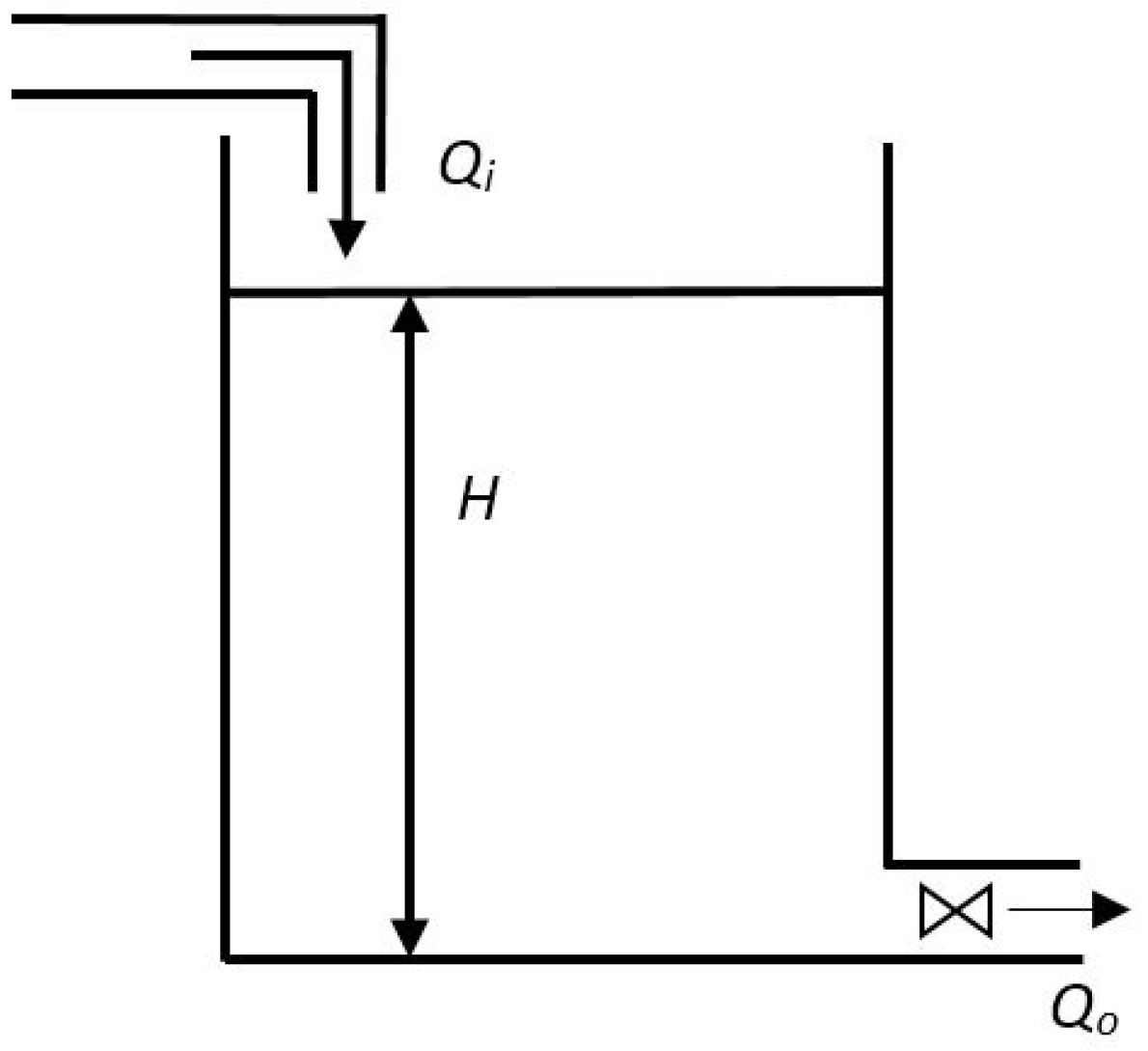
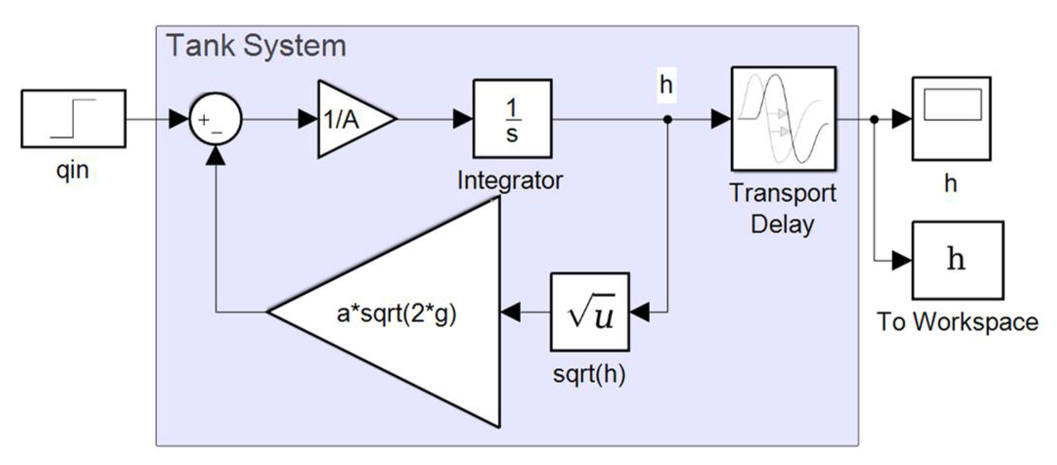
2.1.1. Single Tank Model

Figure 1 shows the single input–single output (SISO) tank system.

Figure 1. ST system.

Considering the mass balance, the dynamic equation of the ST system is [3]:

$$A\frac{dH}{dt}=Q_i-Q_o.$$

(1)

Equation (1) can be written as:

$$A\frac{dH}{dt}=Q_i-\alpha \sqrt{H},$$

(2)

where

$$\alpha =a\sqrt{2g}.$$

(3)

2.1.2. Coupled Tank Model

The CT system consists of two vertical tanks linked by a channel (Figure 2). Each tank has an independent pump for the inflow of liquid. The CT system can be configured as a SISO or MIMO (multiple input–multiple output) system.

Figure 2. CT system.

Using the mass balance equation, the mathematical model of the tank system is derived. The nonlinear equations that describe the dynamics of each tank are:

$$\begin{array}{l}{A}_1\frac{d{H}_1}{dt}=Q_{i1}-Q_{o1}-Q_{o3},\\ A_2\frac{d{H}_2}{dt}=Q_{i2}-Q_{o2}+Q_{o3}.\end{array}$$

(4)

Relation (4) can be written as:

$$\begin{array}{l}{A}_1\frac{d{H}_1}{dt}=Q_{i1}-{\alpha }_1\sqrt{H_1}-{\alpha }_3\sqrt{H_1-H_2},\\ A_2\frac{d{H}_2}{dt}=Q_{i2}-{\alpha }_2\sqrt{H_2}+{\alpha }_3\sqrt{H_1-H_2},\end{array}$$

(5)

where

$${\alpha }_1=a_1^{}\sqrt{2g}, {\alpha }_2=a_2\sqrt{2g}, {\alpha }_3=a_3\sqrt{2g}.$$

(6)

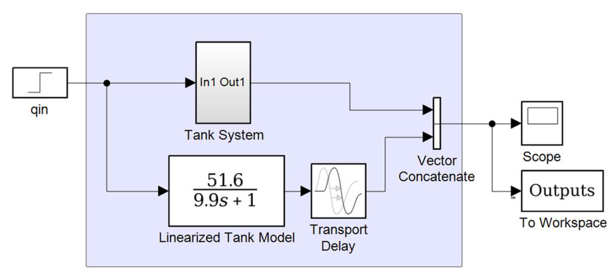
2.2. Model Linearization

2.2.1. Single Tank Model Linearization

Figure 3 shows a SISO tank nonlinear system.

Figure 3. SISO nonlinear tank system.

The ST system is nonlinear due to the square-root term of the liquid height in the tank that appears in the model. Its linearization will be performed based on the recording of its step response. The static gain of the system K, the time constant T_l, and the time delay τ, can be determined from the obtained response curve.

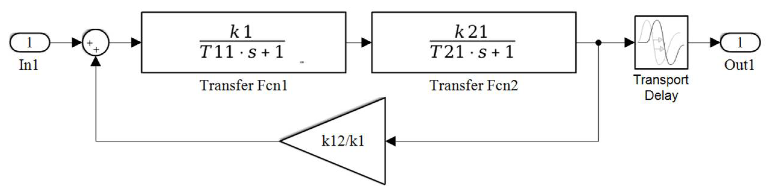
2.2.2. Coupled Tank Model Linearization

The linearization of the CT nonlinear model provided with relation (5) can be performed using the Taylor series method [5,6,7]. Specifically, using the mentioned method around the stationary state, it can be written as follows:

$$\begin{array}{l}\sqrt{H_1}\approx \sqrt{H_{1s}}+\frac{1}{2\sqrt{H_{1s}}}(H_1-H_{1s}),\\ \sqrt{H_2}\approx \sqrt{H_{2s}}+\frac{1}{2\sqrt{H_{2s}}}(H_2-H_{2s}),\\ \sqrt{H_1-H_2}\approx \sqrt{H_{1s}-H_{2s}}+\frac{1}{2\sqrt{H_{1s}-H_{2s}}}\left[(H_1-H_2)-(H_{1s}-H_{2s})\right].\end{array}$$

(7)

Moreover, the following would be valid:

$$\begin{array}{l}0=Q_{i1s}-{\alpha }_1\sqrt{H_{1s}}-{\alpha }_3\sqrt{H_{1s}-H_{2s}},\\ 0=Q_{i2s}-{\alpha }_2\sqrt{H_{2s}}+{\alpha }_3\sqrt{H_{1s}-H_{2s}}.\end{array}$$

(8)

After inserting (7) into (5), and by subtracting (8) from the obtained expression, it is be written as follows:

$$\begin{array}{l}{A}_1\frac{d{H}_1}{dt}=(Q_{i1}-Q_{i1s})-\frac{{\alpha }_1}{2\sqrt{H_{1s}}}(H_1-H_{1s})-\frac{{\alpha }_3}{2\sqrt{H_{1s}-H_{2s}}}\left[(H_1-H_2)-(H_{1s}-H_{2s})\right],\\ A_2\frac{d{H}_2}{dt}=(Q_{i2}-Q_{i2s})-\frac{{\alpha }_2}{2\sqrt{H_{2s}}}(H_2-H_{2s})+\frac{{\alpha }_3}{2\sqrt{H_{1s}-H_{2s}}}\left[(H_1-H_2)-(H_{1s}-H_{2s})\right].\end{array}$$

(9)

By introducing a substitution,

$$\begin{array}{l}{q}_{i1}=Q_{i1}-Q_{i1s}, q_{i2}=Q_{i2}-Q_{i2s},\\ h_1=H_1-H_{1s}{, h}_2=H_2-H_{2s}, \\ h_1-h_2=(H_1-H_2)-(H_{1s}-H_{2s}),\end{array}$$

(10)

It can be written as follows:

$$\begin{array}{l}{A}_1\frac{d{h}_1}{dt}=q_{i1}-\frac{{\alpha }_1}{2\sqrt{H_{1s}}}{h}_1-\frac{{\alpha }_3}{2\sqrt{H_{1s}-H_{2s}}}(h_1-h_2),\\ A_2\frac{d{h}_2}{dt}=q_{i2}-\frac{{\alpha }_2}{2\sqrt{H_{2s}}}{h}_2+\frac{{\alpha }_3}{2\sqrt{H_{1s}-H_{2s}}}(h_1-h_2).\end{array}$$

(11)

Introducing the substitution (12),

$$\begin{array}{l}{T}_{11}=\frac{A_1}{\frac{{\alpha }_1}{2\sqrt{H_{1s}}}+\frac{{\alpha }_3}{2\sqrt{H_{1s}-H_{2s}}}}{, T}_{21}=\frac{A_2}{\frac{{\alpha }_2}{2\sqrt{H_{2s}}}+\frac{{\alpha }_3}{2\sqrt{H_{1s}-H_{2s}}}},\\ k_1=\frac{1}{\frac{{\alpha }_1}{2\sqrt{H_{1s}}}+\frac{{\alpha }_3}{2\sqrt{H_{1s}-H_{2s}}}},k_2=\frac{1}{\frac{{\alpha }_2}{2\sqrt{H_{2s}}}+\frac{{\alpha }_3}{2\sqrt{H_{1s}-H_{2s}}}},\\ k_{12}=\frac{\frac{{\alpha }_3}{2\sqrt{H_{1s}-H_{2s}}}}{\frac{{\alpha }_1}{2\sqrt{H_{1s}}}+\frac{{\alpha }_3}{2\sqrt{H_{1s}-H_{2s}}}}, k_{21}=\frac{\frac{{\alpha }_3}{2\sqrt{H_{1s}-H_{2s}}}}{\frac{{\alpha }_2}{2\sqrt{H_{2s}}}+\frac{{\alpha }_3}{2\sqrt{H_{1s}-H_{2s}}}},\end{array}$$

(12)

relation (11) in the Laplace domain is written as follows:

$$\begin{array}{l}{h}_1(T_{11}s+1)=q_{i1}{k}_1+k_{12}{h}_2,\\ h_2(T_{21}s+1)=q_{i2}{k}_2+k_{21}{h}_1,\end{array}$$

(13)

which is a linearized MIMO CT model.

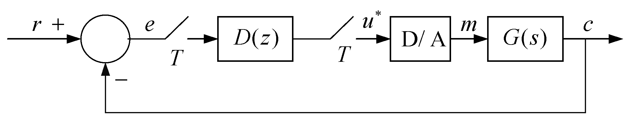
2.3. Controller Design

The control of the tank level is performed using a digital computer. Therefore, two approaches to digital control design are used: The application of the Dahlin algorithm and the design of a digital PID controller, where the PID parameters are adjusted according to the Takahashi PID tuning method.

2.3.1. The Dahlin Controller Design

This algorithm of digital controller parameters setting is applied in the control systems, in which time constants are significantly higher than the transport delay and when it is desired that the controlled variable has an aperiodic response to a step signal at the input in the closed feedback loop [27,28,29,31].

The standard control structure of the Dahlin algorithm is shown in Figure 4, where T is the sampling time, D/A is zero-order hold (ZOH) with the transfer function $G_h(s)=\frac{1-e^{-Ts}}{s}$, and D(z) represents the Dahlin controller.

Figure 4. The control structure of the Dahlin algorithm.

According to this algorithm, the desired aperiodic step response with a time constant of 1/λ and transport delay $T_d=NT$ is adopted as shown in Figure 5.

Figure 5. Desired step response with the Dahlin controller.

The complex form of this response is:

$$C(s)=\frac{\lambda }{s(s+\lambda )}{e}^{-NTs}.$$

(14)

2.3.2. The Dahlin Controller for the Single Tank Model

When the process that is being controlled has the first-order transfer function,

$$G(s)=\frac{K}{T_{l}s+1}{e}^{-\mathsf{\tau }s},$$

(15)

The following dependence between τ and NT is applicable:

$$\mathsf{\tau }=NT+(1-m)T,\hspace{1em}0<m\le 1,$$

(16)

where m is the parameter of the modified Z transformation.

The Dahlin controller has the Z−transform [27,30,31],

$$D(z)=\frac{(1-e^{-\lambda T})\left[1-(e^{-T/T_1})z^{-1}\right]}{K[1-e^{-\lambda T}{z}^{-1}-(1-e^{-\lambda T})z^{-N-1}](C_1+C_2{z}^{-1})},$$

(17)

where

$$C_1=1-e^{-mT/T_1}, C_2=e^{-mT/T_1}-e^{-T/T_1}.$$

(18)

Occasionally, digital controllers provide a control signal that oscillates with a decreasing amplitude in regard to the stationary level. This is known as “ringing” and is caused by a negative, real pole that is close to the “−1” point in the z-plane and the complex conjugate poles within the unit circle. A quick way to avoid ringing, as the authors proposed, is to include z = 1 only in the factor $(C_1+C_2{z}^{-1})$. In this way, the modified Dahlin controller, which should eliminate the effect of sudden changes in the control signal, has the following form:

$$D(z)=\frac{(1-e^{-\lambda T})\left[1-(e^{-T/T_1})z^{-1}\right]}{K[1-e^{-\lambda T}{z}^{-1}-(1-e^{-\lambda T})z^{-N-1}](C_1+C_2)}.$$

(19)

The control law for non-ringing control signals can also be written as the control law of a digital PI regulator. The transfer function of the Dahlin PI controller is [30]:

$$D(z)=K_P\left[1+\frac{T/T_I}{1-z^{-1}}\right],$$

(20)

$$K_P=\frac{1-e^{-\lambda T}}{K(e^{T/T_1}-1)[1+N(1-e^{-\lambda T})]}, T/T_I=e^{-T/T_1}-1.$$

(21)

2.3.3. The Dahlin Controller for the Coupled Tank Model

When a process has the second-order transfer function,

$$G(s)=\frac{K}{(T_{l}s+1)(T_{2}s+1)}{e}^{-NTs},$$

(22)

The Dahlin controller has the Z−transform [31], as follows:

$$D(z)=\frac{(1-e^{-\lambda T})\left[1-(e^{-T/T_1})z^{-1}\right]\left[1-(e^{-T/T_2})z^{-1}\right]}{K[1-e^{-\lambda T}{z}^{-1}-(1-e^{-\lambda T})z^{-N-1}](C_3+C_4{z}^{-1})},$$

(23)

where

$$C_3=1+\frac{T_1{e}^{-T/T_1}-T_2{e}^{-T/T_2}}{T_2-T_1}, C_4=e^{-T/T_1}{e}^{-T/T_2}+\frac{T_1{e}^{-T/T_2}-T_2{e}^{-T/T_1}}{T_2-T_1}.$$

(24)

A possible way to avoid ringing of the control signal of the Dahlin controller (23), which is designed for the system described with the transfer function (22), is to include z = 1 in the factors $[1+(1-e^{-\lambda T})z^{-1}](C_3+C_4{z}^{-1})$ of the denominator in the Dahlin controller transfer function [27,30,31]. For N = 1, this modified Dahlin controller, which can eliminate the effect of sudden changes in the control signal, has the following form:

$$D(z)=\frac{(1-e^{-\lambda T})\left[1-(e^{-T/T_1})z^{-1}\right]\left[1-(e^{-T/T_2})z^{-1}\right]}{K(2-e^{-\lambda T})(C_3+C_4)(1-z^{-1})}.$$

(25)

The control law (25) for arbitrary N can be written as the control law of a digital PID regulator. PID controller expressed via Dahlin algorithm is as follows:

$$D(z)=K_P\left[1+\frac{T/T_I}{1-z^{-1}}+\frac{T_D}{T}(1-z^{-1})\right],$$

(26)

where

$$\begin{array}{c}{K}_P=\frac{(1-e^{-\lambda T})\left[e^{T/T_1}+e^{T/T_2}-2\right]}{K(e^{T/T_1}-1)(e^{T/T_2}-1)[1+N(1-e^{-\lambda T})]},\\ \\ \frac{T}{T_I}=\frac{(e^{T/T_1}-1)(e^{T/T_2}-1)}{e^{T/T_1}+e^{T/T_2}-2}, \frac{T_D}{T}=\frac{1}{e^{T/T_1}+e^{T/T_2}-2}.\end{array}$$

(27)

2.3.4. The PID Controller Design

The general form of analog and digital PID controllers is:

$$\begin{array}{l}G(s)=K_P+\frac{K_I}{s}+K_{D}s,\\ G(z)=K_P+\frac{K_I}{1-z^{-1}}+K_D(1-z^{-1}).\end{array}$$

(28)

To design PID controllers, the Ziegler–Nichols method (for continuous controllers) and the Takahashi method (for discrete controllers) were used, as shown in Table 1. These methods also assume that parameters K_Pkr and T_kr have been previously determined in a closed-loop experiment.

Table 1. The PID controller parameter selection [32].

Ziegler–Nichols Method
KP	KI	KD
0.5 KPkr	-	-
0.45 KPkr	KP1.2/Tkr	-
0.6 KPkr	KP 2/Tkr	KP 0.125 Tkr
Takahashi method
KP	KI	KD
0.5 KPkr	-	-
0.45 KPkr − 0.5 KI	0.54 KPkrT/Tkr	-
0.6 KPkr − 0.5 KI	1.2 KPkrT/Tkr	3/40 KPkrTkr/T

3. Results

3.1. Single Tank Control Results

3.1.1. Single Tank Model Linearization

The linearization of the ST system shown in Figure 3 is based on the recording of its step response in Figure 6, where the adopted system parameter values are presented in Table 2.

Figure 6. The step response of the ST system.

Table 2. ST parameters.

Symbol	Value	Unit
a	0.0134	m2
A	0.1257	m2

As can be seen in Figure 6, the static gain of the system K and the time constant T_l, which is inversely proportional to the steepest tangent of the system step response and the time delay τ, can be determined. Therefore, we can obtain the linearized tank transfer function in the following form:

$$G(s)=\frac{K}{T_{l}s+1}{e}^{-\mathsf{\tau }s}=\frac{51.6}{9.9s+1}{e}^{-4.3s}.$$

(29)

In addition, it can be seen that the rise time, defined as the time for the response signal to increase from 0.1 to 0.9 of its final value, is T_r = 25.91 s.

To confirm the model linearization procedure, the responses of the nonlinear tank system shown in Figure 3 and the resulting linearized model provided with relation (29) are compared in Figure 7.

Figure 7. The Simulink model of the tank system and the linearized tank model.

The responses of the tank system and the linearized tank model, which largely coincide, confirm the validity of the applied procedure as shown in Figure 8.

Figure 8. The comparison of the ST system and the linearized ST model responses.

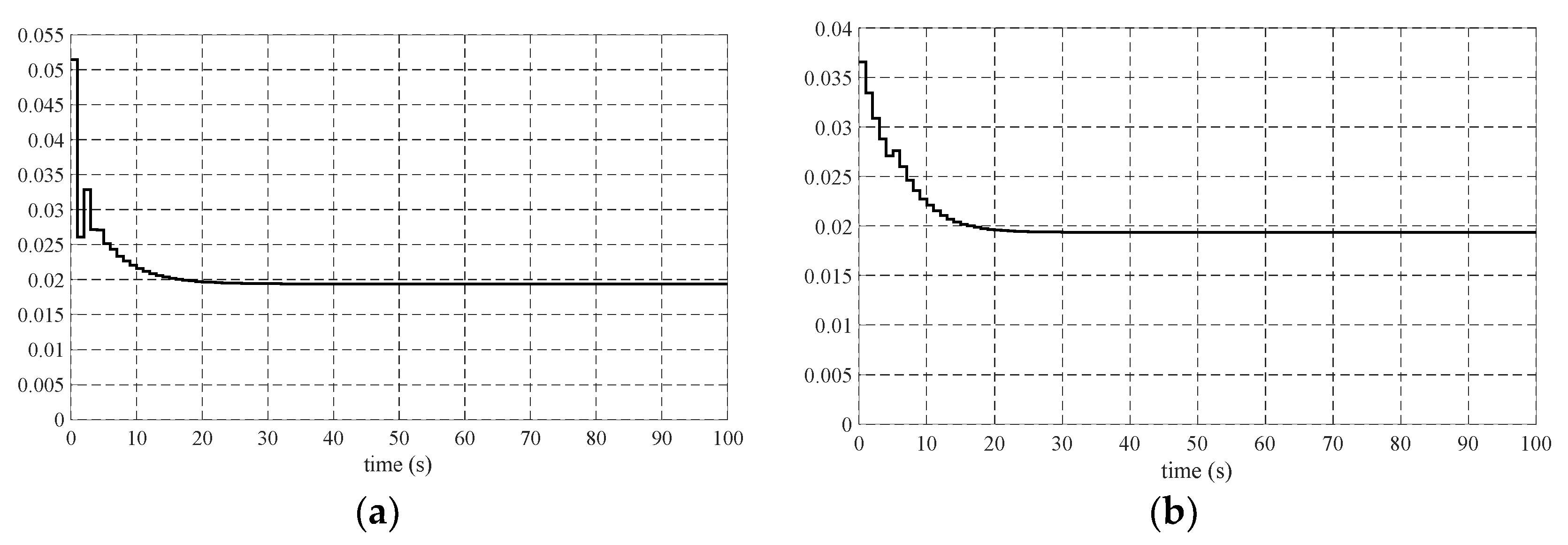
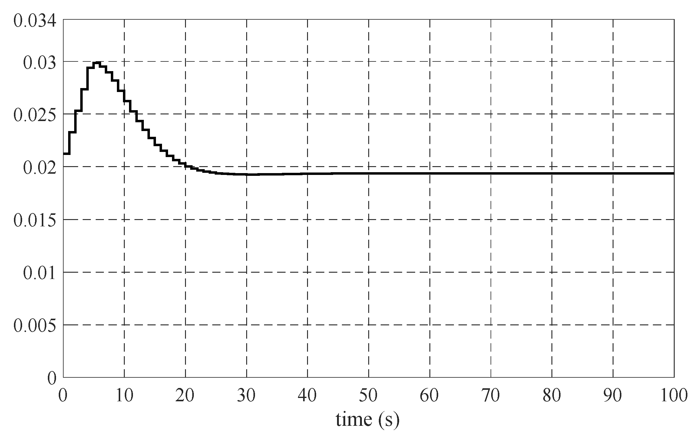
3.1.2. The Dahlin Algorithm Results

Let the chosen sampling period be $T=1 \mathrm{s}$. Since the transport delay for the single-tank system is $\mathsf{\tau }=4.3 \mathrm{s}$ and the sampling period is T = 1 s, from (16) it follows that $m=0.7$ and $N=4$.

Let the time constant of the desired aperiodic response be $1/\lambda =5 \mathrm{s}$.

Based on the parameters presented in Table 2, relation (17) is written as follows:

$$D(z)=\frac{0.181\cdot (1-0.904\cdot z^{-1})}{51.6\cdot (1-0.819\cdot z^{-1}-0.181\cdot z^{-5})\cdot (0.068+0.028\cdot z^{-1})}.$$

(30)

Figure 9 shows the Simulink model of the tank system with the Dahlin controller. The height of the liquid in the ST system with the Dahlin controller is shown in Figure 10.

Figure 9. The Simulink model of the ST system with the Dahlin controller.

Figure 10. The output of the ST system with the Dahlin controller.

The obtained output has a desired response time of 5 s and an expected delay time of 4 s. The expected aperiodic output with no oscillation and no overshoot was achieved, with a rise time of T_r = 10.8 s and a setting time of T_s = 20 s, Table 3.

Table 3. Parameters of the transient response with the Dahlin controller.

Parameters	Dahlin Algorithm
Rise time	10.8 s
Overshoot	0
Setting time	20 s
Steady-state error	0

The transfer function of the modified Dahlin controller with “no ringing” effect of the control signal, based on (19), is:

$$D(z)=\frac{0.1813z^5-0.1639z^4}{4.958z^5-4.059z^4-0.8986}.$$

(31)

Control signals from the Dahlin controller with the effect of “ringing” and from the modified Dahlin controller with “non-ringing” behavior are shown in Figure 11. The control signal from the Dahlin PI control is presented in Figure 12.

Figure 11. Control signals from: (a) The Dahlin controller with ringing; (b) The modified Dahlin controller with non-ringing, for ST system.

Figure 12. A control signal from the Dahlin PI controller.

The transfer function of the Dahlin PI controller, based on (20) and (21), is:

$$D(z)=0.0192\left(1+\frac{0.1063}{1-z^{-1}}\right).$$

(32)

Figure 13 shows the responses obtained from the designed controllers. The response obtained with the modified Dahlin controller matches the response obtained with the Dahlin controller. However, the response obtained with the Dahlin PI controller somewhat deviates from these responses. It has an overshoot of P% = 3.8%, rise time of T_r = 11 s, and a setting time of T_s = 29 s.

Figure 13. The output of the ST system with Dahlin controllers.

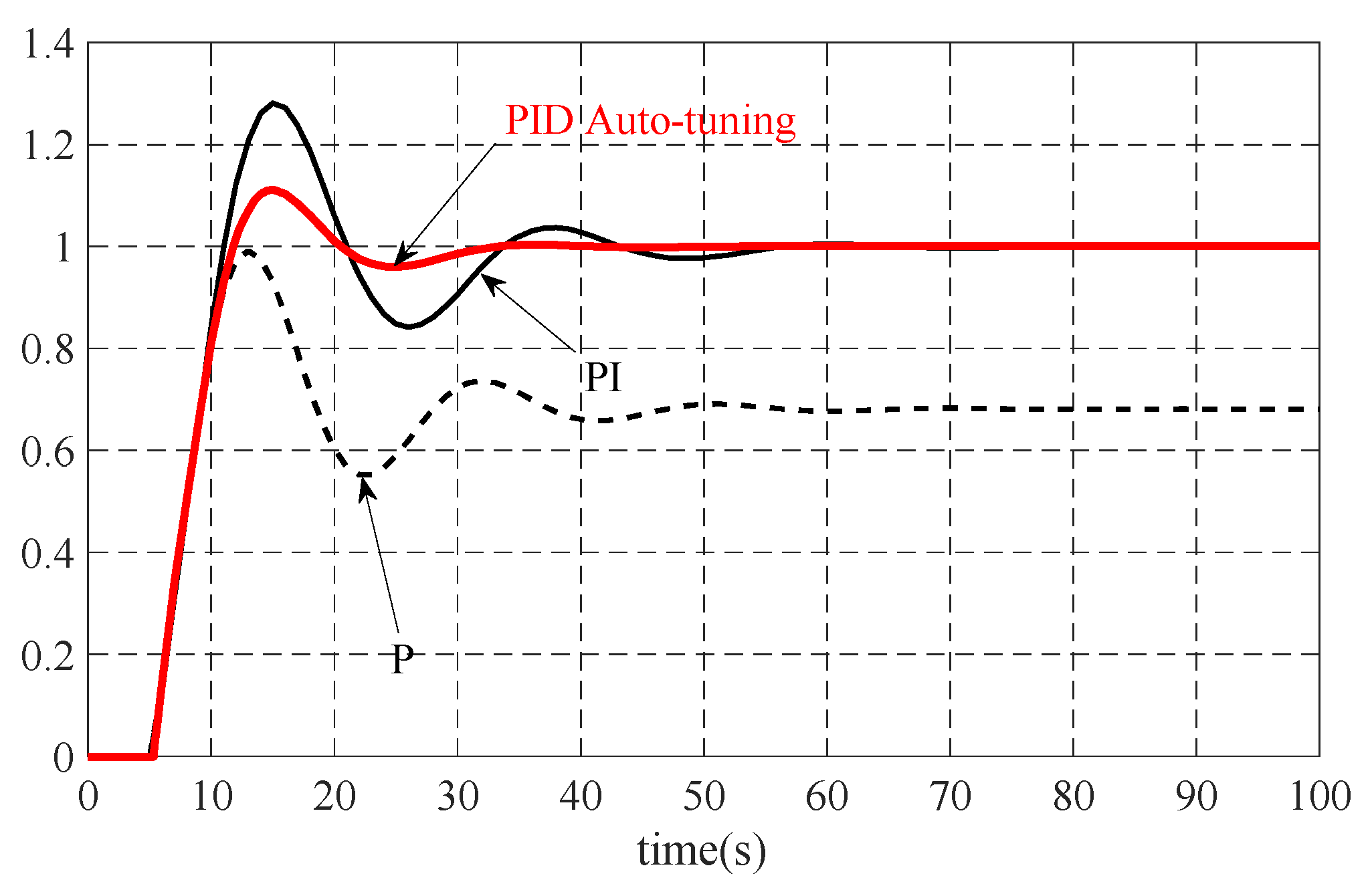
3.1.3. The PID Control Results

Figure 14 and Figure 15 show the output of the ST system with PID controllers obtained using Ziegler–Nichols, Takahashi, and Auto-tuning methods.

Figure 14. The output of the ST system with PID controller using Ziegler–Nichols and Auto-tuning methods.

Figure 15. The output of the ST system with PID controller and Takahashi method.

To obtain the PID parameters presented in Table 1, it was necessary to determine K_Pkr and T_kr by gradually increasing K_P until an undamped response is reached. The reached gain value of K_P is called the critical gain K_Pkr and the time between two adjacent maxima is the critical oscillation period T_kr as shown in Figure 16.

Figure 16. Derivation of K_pkr and T_kr.

The selection of the PID controller parameters using the Ziegler–Nichols, Takahashi tuning, and Auto-tuning methods is presented in Table 4.

Table 4. PID controller parameter selection for the ST system.

Ziegler–Nichols Method
KP	KI	KD
2.135	-	-
1.9215	0.1537	-
2.5620	0.3416	4.8038
Takahashi tuning method
KP	KI	KD
2.135	-	-
1.845	0.1537	-
2.3912	0.3416	4.8038
Auto-tuning method
KP	KI	KD
1.554	0.147	1.2445

The parameters of the transient response with PID controllers are shown in Table 5. The choice of PID controller parameters using the Ziegler–Nichols method is not presented in Table 5, since it provided an extremely oscillating response.

Table 5. The parameters of the transient response with PID controllers.

Controller		Rise Time	Overshoot	Setting Time	Steady-State Error
Ziegler–Nichols method	P	4.7 s	45.58%	38 s	0.31
	PI	5.65 s	23.2%	30.2 s	0
Takahashi method	P	4.8 s	45.76%	42 s	0.32
	PI	9.2 s	23%	38 s	0
	PID	3.2 s	61.8%	46 s	0
Auto-tuning method	PID	4.87 s	14.3%	26.7 s	0

Based on the parameters shown in Table 5, it can be concluded that the best transient response parameters provided the Auto-tuning method as well as the PI controllers with parameters selected by the Ziegler–Nichols and Takahashi tuning methods.

3.2. The Coupled Tank Control Results

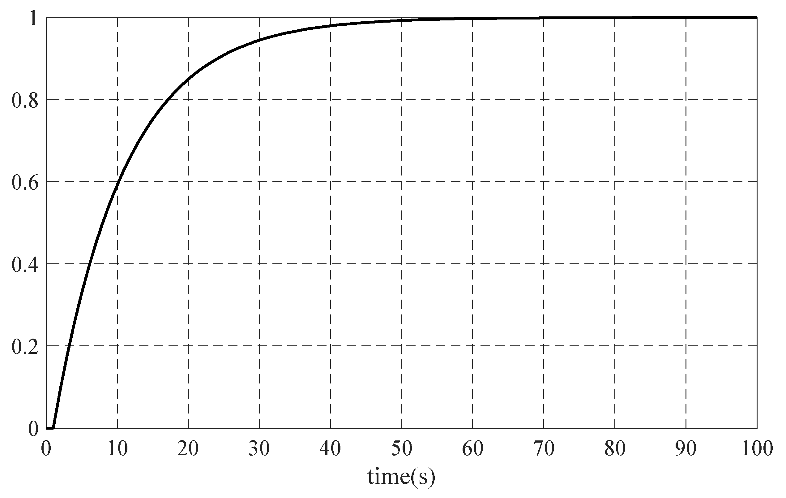
3.2.1. The Coupled Tank Model Linearization

Table 6 shows the adopted parameters of the CT system.

Table 6. Coupled tank system parameters.

Symbol	Value	Unit
H1s	2.5	m
H2s	1.5	m
a1	58.088 × 10−4	m2
a2	63.6173 × 10−4	m2
a3	72.3823 × 10−4	m2
A1	2.0106	m2
A2	1.7908	m2

If we assume that $q_{i2}=0,$ in relaton (13), then the CT linearized SISO model can be derived as shown in Figure 17.

Figure 17. The CT linearized SISO model.

The transfer function of the CT model can be described by the following equation:

$$G(s)=\frac{h_2(s)}{q_{i1}(s)}=\frac{K}{(T_{l}s+1)(T_{2}s+1)}{e}^{-\mathsf{\tau }s}.$$

(33)

Using the data presented in Table 6, relation (33), and the model in Figure 17, the linearized transfer function of the CT system is written as as follows:

$$G(s)=\frac{h_2(s)}{q_{i1}(s)}=\frac{0.0039}{(44.84s+1)(196.08s+1)}{e}^{-s}.$$

(34)

The linearized CT model response is shown in Figure 18.

Figure 18. The linearized CT model response.

3.2.2. The Dahlin Algorithm

Let the chosen sampling period be $T=1 \mathrm{s}$, and the time constant of the desired aperiodic response be $1/\lambda =10 \mathrm{s}$. Then, the transport delay for the CT system is $\mathsf{\tau }=1 \mathrm{s}$.

Based on the system parameters presented in Table 6 and relation (23), the transfer function of the Dahlin controller is:

$$D(z)=\frac{4.3027\cdot {10}^5\cdot (1-0.9779\cdot z^{-1})\cdot (1-0.9949\cdot z^{-1})}{(1-0.9048\cdot z^{-1}-0.09516\cdot z^{-2})\cdot (1+0.9909\cdot z^{-1})}.$$

(35)

The Simulink model and the output of the CT system with the Dahlin controller are shown in Figure 19 and Figure 20, respectively.

Figure 19. The Simulink model of the CT system with the Dahlin controller.

Figure 20. The output of the CT system with the Dahlin controller.

The transfer function of the modified Dahlin controller with the “no ringing” effect of the control signal, based on (25), is:

$$D(z)=\frac{1.9734\cdot {10}^5\cdot (1-0.9906\cdot z^{-1})\cdot (1-0.9926\cdot z^{-1})}{1-z^{-1}}.$$

(36)

Control signals from the Dahlin controller with the effect of “ringing” and from the modified Dahlin controller with “non-ringing” behavior are shown in Figure 21.

Figure 21. Control signals from: (a) The Dahlin controller with ringing; (b) The modified Dahlin controller with non-ringing, for CT system.

The transfer function of the Dahlin PID controller, which is the variant of the modified Dahlin controller, based on (26) and (27), is:

$$D(z)=5.3115\cdot {10}^3\left[1+\frac{0.0042}{1-z^{-1}}+36.148\cdot (1-z^{-1})\right].$$

(37)

The outputs of the CT system with the different Dahlin controllers are presented in Figure 22.

Figure 22. The outputs of the CT system with the different Dahlin controllers.

The obtained output of the coupled tank system with the Dahlin controller has a given response time of 10 s and an expected delay time of 1 s. The expected aperiodic output with no oscillation and no overshoot was achieved, with a rise time of T_r = 21 s and setting time of T_s = 41 s as shown in Table 7.

Table 7. The parameters of the transient response with the Dahlin controller.

Parameters	Dahlin Algorithm
Rise time	21 s
Overshoot	0
Setting time	41 s
Steady-state error	0

Control signals from the modified Dahlin controller and the Dahlin PID controller are shown in Figure 23.

Figure 23. Control signals from the modified Dahlin controller and the Dahlin PID controller.

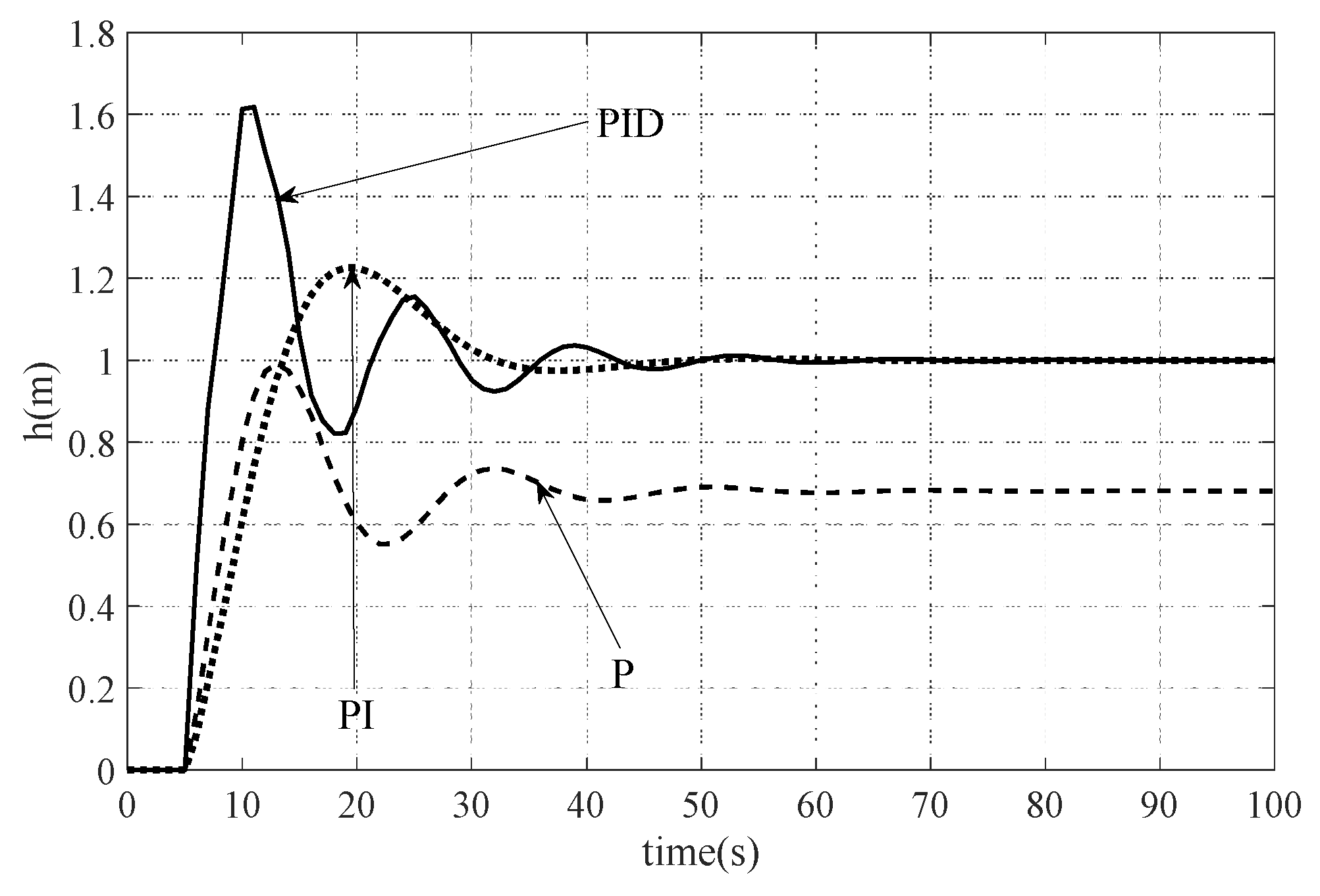
3.2.3. The PID Control Results

Figure 24 and Figure 25 show the output of the CT system with PID controller using the Ziegler–Nichols, Takahashi, and Auto-tuning methods.

Figure 24. The output of the CT system with PID controller using the Ziegler–Nichols and continuous Auto-tuning methods.

Figure 25. The output of the CT system with PID controller using the Takahashi and discrete Auto-tuning methods.

Figure 26 shows the derivation of K_pkr and T_kr for the CT system.

Figure 26. The derivation of K_pkr and T_kr for the CT system.

The selection of the PID controller parameters using the various variants of the PID controllers is shown in Table 8. C and D represent the continuous and discrete Auto-tuning approaches, respectively.

Table 8. PID controller parameter selection for the CT system.

Ziegler–Nichols Method
KP		KI	KD
121		0	0
108.9		3.4389	0
145.2		7.6421	689.7
Takahashi tuning method
KP		KI	KD
121		0	0
107.1805		3.4389
141.3789		7.6421	689.7
Auto-tuning method
KP		KI	KD
C	110.452	1.479	1896.5737
D	35.2523	0.30011	804.0765

The parameters of the transient response with PID controllers are shown in Table 9. The choice of PI controller parameters using the Ziegler–Nichols and the Takahashi tuning methods are not presented in Table 9, since they provided a non-stable response.

Table 9. The transient response parameters with the PID controllers.

Controller			Rise Time	Overshoot	Setting Time	Steady-State Error
Ziegler–Nichols method	P		9.34 s	83.2%	567 s	0
	PID		7.27 s	66.5%	233 s	0
Takahashi method	P		9 s	91.3%	1140 s	0
	PID		8 s	71.7%	347 s	0
Auto-tuning method	PID	C	5.78 s	9.69%	59.1 s	0
		D	16 s	8.7%	107 s	0

In this case, the best results provided the use of the PID controller with parameters selected by the continuous Auto-tuning, Ziegler–Nichols, and Takahashi tuning methods.

4. Discussion

This paper presents the level control of the ST and CT. For this purpose, it was necessary to design different controllers. In particular, the Dahlin controller and standard PID controllers were used.

Both systems are nonlinear. In order to design the controllers, it was necessary to linearize them. As a result, different approaches to model linearization were applied. In the case of a ST system, the authors suggest that linearization should be performed based on the obtained system response curve. The gain factor, the time constant, and the transport delay can be easily determined from the recorded curve. In the case of higher-order systems, we propose linearization by development into the Taylor series.

The Dahlin algorithm applied for both tank systems control provides very good results. The application of the Dahlin controller enables the aperiodic response of the system with the desired time constant. The problem with using this controller can be the sudden change in the control signal, which is difficult to follow for most actuators. According to Dahlin, this problem can be effectively overcome by eliminating three poles, namely, a pair of complex conjugate poles and one real negative pole within the unit circle. In this way, a modified Dahlin controller is designed, which provides a very similar response as the Dahlin controller, but a control signal with “non-ringing” behavior.

In the first-order system, the elimination of the mentioned three poles is relatively simple if the system has a transport delay of about 2 s, i.e., N = 2. In this case, the modified Dahlin controller becomes a Dahlin PI controller. However, in the case of a system with the transport delay greater than 2, i.e., N greater than 2, the elimination of these three poles becomes more difficult. In this case, Dahlin suggests the design of a Dahlin PI controller [30]. This controller, in the example of a single tank, when N = 4, did not provide satisfactory results. The desired aperiodic response was not achieved, but a response with an overshoot as shown in Figure 13, although the sudden changes in the control signal were eliminated as presented in Figure 12. Therefore, the authors propose the elimination of only one pole, namely, the real negative pole, by including z = 1 in the factor $(C_1+C_2{z}^{-1})$, (19), (31). The proposed modified Dahlin controller provided very good results for a ST system. The response almost matched the Dahlin controller, and the ringing of the control signal was eliminated as shown in Figure 11b and Figure 13.

In the second-order system, the elimination of the three mentioned poles can be effectively carried out if N = 1, which was the case with the analyzed example of a CT system. The modified (“non-ringing”) control signal from the Dahlin controller, matched the control signal from the Dahlin PID controller as shown in Figure 23, and the desired aperiodic response was achieved as presented in Figure 22. For systems when N is greater than 1, the authors propose the application of only the elimination of one negative pole by including z = 1 in the factor $(C_3+C_4{z}^{-1})$.

4.1. The Transient Response Performances

Table 10 and Table 11 show the parameters of the transient response with the implementation of different controllers (Dahlin—D, modified Dahlin—MD, Ziegler–Nichols—ZN, Takahashi—T, and Auto-tuning—AT) in the analyzed systems.

Table 10. The parameters of the transient response with different controllers in the ST system.

Parameters	D	MD	D PI	PI ZN	PI T	PID AT
Rise time	10.8 s	10.8 s	11 s	5.65 s	9.2 s	4.87 s
Overshoot	0	0	3.8%	23.2%	23%	14.3%
Setting time	20 s	20 s	29	30.2 s	38 s	26.7 s
Steady-state error	0	0	0	0	0	0

Table 11. The parameters of the transient response with different controllers in the CT system.

Parameters	D	MD	D PID	PID ZN	PID T	PID AT
Rise time	21 s	21 s	21 s	7.27 s	14.6 s	5.78 s
Overshoot	0	0	0	66.5%	16%	9.69%
Setting time	41 s	41 s	41 s	233 s	82.4 s	59.1 s
Steady-state error	0	0	0	0	0	0

In comparison to the application of the Dahlin controller, standard procedures based on the Ziegler–Nichols, Takahashi, and Auto-tuning methods, provided responses with an overshoot and longer setting time. Only the rise time was slightly shorter with the use of standard PID controllers as shown in Table 10 and Table 11.

Moreover, the modified Dahlin controller always provides stability, with no error in the aperiodic response and a “non-ringing” control signal, which is not the case when applying standard PID controllers.

4.2. The Comparison of the Performance Indexes

Table 12, Table 13, Table 14 and Table 15 present various performance indexes, such as integral error (IE);integral of the absolute error (IAE); integral of the square error (ISE); integral of time-weighted absolute error (ITAE); integral of time square error (ITASE) of PID and Dahlin controller, considering a 1000 s simulation time.

Table 12. Performance evaluation of PID controller in the ST system.

Controller		IE	IAE	ISE	ITAE	ITASE
Ziegler–Nichols method	P	321.5	321.5	106.5	1595 × 105	1595 × 105
	PI	6.505	10.57	6.693	116.9	40.63
	PID	2927	6.58 × 1014	2.517 × 1028	1.011 × 1016	1.956 × 1015
Takahashi method	P	321.5	321.5	106.5	1595 × 105	1595 × 105
	PI	6.606	10.7	6.726	119.2	30.75
	PID	2.425	10.21	6.44	111	−11.56
Auto-tuning method	PID	6.084	8.022	6.119	52.31	32.75

Table 13. Performance evaluation of Dahlin controller in the ST system.

Controller		IE	IAE	ISE	ITAE	ITASE
Dahlin	1/λ = 5 s	8.366	9.639	6.55	395.1	−272.1
Modified Dahlin	1/λ = 5 s	9.465	9.465	6.77	273	273
Dahlin	1/λ = 4 s	7.462	8.519	6.059	320.1	−225.5
Modified Dahlin	1/λ = 4 s	8.004	8.02	6.286	37.62	37.09

Table 14. Performance evaluation of PID controller in the CT system.

Controller			IE	IAE	ISE	ITAE	ITASE
Ziegler–Nichols method		P	10.15	96.27	37.7	1.548 × 104	4026
		PID	0.1309	38.07	14.62	2370	−29.02
Takahashi method		P	9.583	180.9	73.57	4.709 × 104	3948
		PID	−0.3729	49.45	19.96	3765	−29.73
Auto-tuning method	C	PID	0.6761	7.228	2.944	140.1	−111.9
	D	PID	2.829	14.04	5.83	520.5	−405.8

Table 15. Performance evaluation of Dahlin controller in the CT system.

Controller		IE	IAE	ISE	ITAE	ITASE
Dahlin	1/λ = 10 s	11.38	11.38	6.046	305.7	305.7
Modified Dahlin	1/λ = 10 s	10.96	11.06	6.364	116.1	89.88
Dahlin	1/λ = 4 s	5.07	5.178	3.081	30.42	16.02
Modified Dahlin	1/λ = 4 s	5.008	5.077	3.501	23.38	10.45

Additionally, Table 13 and Table 15 show the results of the performance evaluation for the Dahlin controller, for different values of the assigned time constant, 1/λ. The authors have determined the lower limit of the decrease in the desired time constant 1/λ, which is 4 T. Decreasing this constant below this limit, as the authors have noted, will not result in the desired behavior.

Regarding the IE, IAE, ISE, ITAE, and ITASE parameters, the best results were almost always obtained using the modified Dahlin controller both in the ST and CT systems.

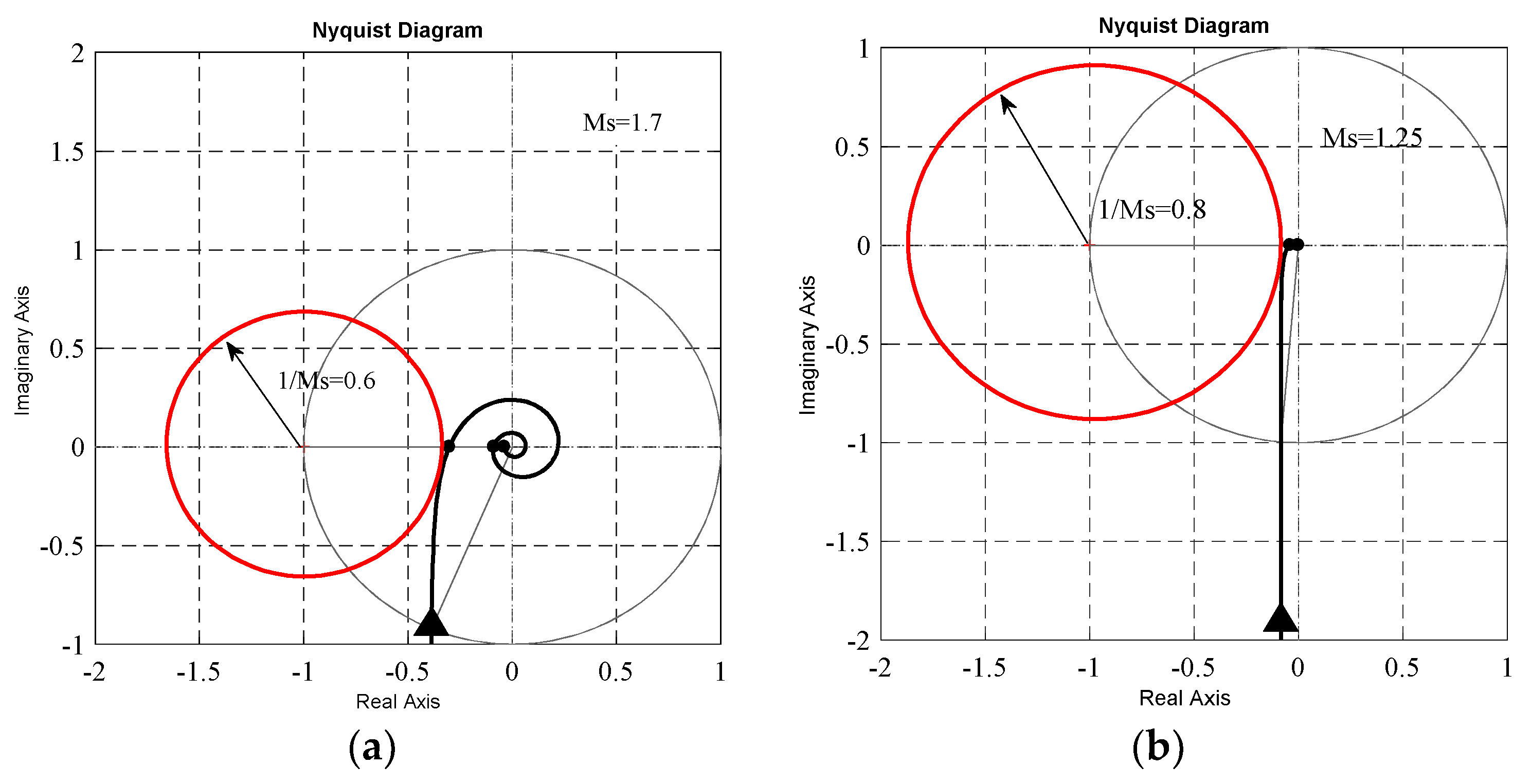
4.3. Robustness Analysis

The robustness of the studied systems with the application of the proposed modified Dahlin controllers is analyzed by the maximum sensitivity M_s, described with (38):

$$M_s=\underset{0\le \mathsf{\omega }<\infty }{\max }\left|\frac{1}{1+G_p(j\mathsf{\omega })G_c(j\mathsf{\omega })}\right|=\underset{0\le \mathsf{\omega }<\infty }{\max }\left|S(j\mathsf{\omega })\right|.$$

(38)

This parameter, in fact, represents the inverse value of the shortest distance of the Nyquist curve from the critical point −1 [11]. Recommended values that characterize good robustness are between 1.2 and 2.

Based on the obtained M_s value, M_s = 1.7 for the ST system, i.e., M_s = 1.25 for the DT systems (Figure 27), it can be concluded that the application of the modified Dahlin controller ensures the high-quality robustness of the systems.

Figure 27. The Nyquist curve for: (a) The ST system; (b) the CT system with modified Dahlin controllers.

4.4. Comparison with Results Provided in the Literature

Another confirmation of the advantage of using the modified Dahlin controller was provided by comparing the obtained results with the results of other authors, through the comparison of performance indexes and the transient response performances. We used their transfer functions of horizontal and vertical CT systems to design the modified Dahlin controller, and additionally determined performance indexes, which were not performed in their works as shown in Table 16, Table 17 and Table 18.

Table 16. Performance of the transient response for the CT system reported in [7].

Parameters	Trial and Error [7]	Auto-Tuning [7]	Ziegler–Nichols [7]	Cohen–Coon [7]	Modified Dahlin 1/λ = 4 s
Rise time	24 s	9.14 s	3.29 s	2.81 s	5 s
Overshoot	6.86%	1.81%	38.5%	33.7%	0%
Setting time	84.4 s	53.3 s	32.1 s	23.59 s	7 s
Steady-state error	0	0	0	0	0

Table 17. Performance evaluation determined from [7].

Methods	Trial and Error	Auto− Tuning	Ziegler– Nichols	Cohen– Coon	Modified Dahlin 1/λ = 4 s
IE	14.24	9.246	0.4068	0.4198	5.009
IAE	16.95	9.272	6.036	4.28	5.009
ISE	10.21	4.783	2.371	1/836	2.787
ITAE	259.5	188.4	58.77	26.58	22.46
ITASE	81.45	188.4	−7.552	−6.886	22.46

Table 18. Performance evaluation determined from [6].

Methods	Ziegler– Nichols	Ciancone Correlation	Pole Placement	Modified Dahlin 1/λ = 4 s
IE	0.4115	1.027	0.4274	5.017
IAE	32.87	78.39	153.6	5.017
ISE	13.69	31.27	60.7	2.789
ITAE	1597	9507	3.538 × 104	22.69
ITASE	−27.94	−71.95	38.93	22.69

5. Conclusions

In this paper, the Dahlin algorithm was used for the level control in single tank and coupled tank systems for the first time. Both systems are nonlinear but were effectively linearized with the proposed procedures. A simple modification of the Dahlin controller resulted in a “non-ringing” control signal and a stable, error-free, aperiodic response of the desired dynamics. Additionally, the lower limit of the decrease in the desired time constant, which ensures the desired behavior of the system, is determined. A comparison of the proposed controller with the PID controllers, which are usually applied, are represented through transient responses and performance indexes. The provided MATLAB Simulink simulations indicate that the proposed modified Dahlin controller has more advantages than the conventional PID controllers.

In the future, special attention will be paid to the application of the experimental validation of the obtained results and the application of the metaheuristic algorithms to estimate optimal PID controller parameters. Furthermore, attention will be paid to the testing of the control system robustness in terms of tank dimension.

References

- Sabri, L.; Al-mshat, H. Implementation of Fuzzy and PID Controller to Water Level System Using LabView. Int. J. Comput. Appl. 2015, 116, 6–10. [Google Scholar] [CrossRef]
- Urrea, C.; Garcia-Garcia, Y. Design and Performance Analysis of Level Control Strategies in a Nonlinear Spherical Tank. Processes 2023, 11, 720. [Google Scholar] [CrossRef]
- Rajput, K.; Giri, V.K. Virtual Instrument Based Liquid Level Control System. Int. J. Adv. Res. Electr. Electron. Instrum. Eng. 2015, 4, 5911–5916. [Google Scholar] [CrossRef]
- Getu, B.N. Water Level Controlling System Using Pid Controller. Int. J. Appl. Eng. Res. 2016, 11, 11223–11227. [Google Scholar]
- Khalid, M.U.; Kadri, M.B. Liquid Level Control of Nonlinear Coupled Tanks System Using Linear Model Predictive Control. In Proceedings of the 2012 International Conference on Emerging Technologies, Islamabad, Pakistan, 8–9 October 2012. [Google Scholar] [CrossRef]
- Tijjani, A.; Shehu, M.; Alsabari, A.; Sambo, Y.; Tanko, N. Performance Analysis for Coupled-Tank System Liquid Level Control Using MPC, PI and PI-plus-Feedforward Control Scheme. J. Robot. Autom. 2017, 1, 42–53. [Google Scholar] [CrossRef]
- Jaafar, H.I.; Hussien, S.Y.; Selamat, N.A.; Aras, M.; Rashid, M.Z. Development of PID Controller for Controlling Desired Level of Coupled Tank System. Int. J. Innov. Technol. Explor. Eng. 2014, 3, 32–36. [Google Scholar]
- Urrea, C.; Páez, F. Design and Comparison of Strategies for Level Control in a Nonlinear Tank. Processes 2021, 9, 735. [Google Scholar] [CrossRef]
- Krata, P.; Wawrzyński, W.; Więckiewicz, W.; Jachowski, J. Ship’s Ballast Tanks Size and Dimensions Review for the Purpose of Model Research into the Liquid Sloshing Phenomenon. Zesz. Nauk. Akad. Morska W Szczec. 2012, 29, 88–94. [Google Scholar]
- Zhao, Z.; Zhang, X.; Li, Z. Tank-Level Control of Liquefied Natural Gas Carrier Based on Gaussian Function Nonlinear Decoration. J. Mar. Sci. Eng. 2020, 8, 695. [Google Scholar] [CrossRef]
- Buljevic, A.; Miletic, M.; Mitrovic, A.; Kapetina, M.; Rapaic, M. Examples of Robust Controller Design. Serb. J. Electr. Eng. 2020, 17, 65–82. [Google Scholar] [CrossRef]
- Dlabač, T.; Ćalasan, M.; Krčum, M.; Marvučić, N. PSO-Based PID Controller Design for Ship Course-Keeping Autopilot. Brodogradnja 2019, 70, 1–15. [Google Scholar] [CrossRef]
- Bozic, M.; Antic, S.; Vujičić, V.; Bjekić, M.; Djordjevic, G. Electronic Gearing of Two DC Motor Shafts for Wheg Type Mobile Robot. FU Elec. Energ. 2018, 31, 75–87. [Google Scholar] [CrossRef]
- Vinod, J.; Sarkar, B.K. Francis turbine electrohydraulic inlet guide vane control by artificial neural network 2 degree-of-freedom PID controller with actuator fault. Proc. Inst. Mech. Eng. Part I J. Syst. Control. Eng. 2021, 235, 1494–1509. [Google Scholar] [CrossRef]
- Venkaiah, P.; Sarkar, B.K. Electrohydraulic Proportional Valve-Controlled Vane Type Semi-Rotary Actuated Wind Turbine Control by Feedforward Fractional-Order Feedback Controller. Proc. Inst. Mech. Eng. Part I J. Syst. Control. Eng. 2022, 236, 318–337. [Google Scholar] [CrossRef]
- Zhang, R.; Gao, L. The Brushless DC Motor Control System Based on Neural Network Fuzzy PID Control of Power Electronics Technology. Optik 2022, 271, 169879. [Google Scholar] [CrossRef]
- Han, J.; Shan, X.; Liu, H.; Xiao, J.; Huang, T. Fuzzy Gain Scheduling PID Control of a Hybrid Robot Based on Dynamic Characteristics. Mech. Mach. Theory 2023, 184, 105283. [Google Scholar] [CrossRef]
- Short, M.; Selvakumar, A.A. Non-Linear Tank Level Control for Industrial Applications. Appl. Math. 2020, 11, 876–889. [Google Scholar] [CrossRef]
- Imaduddin, M.; Kamil, M.A.N.; Putra, S.H.; Imawan, R.; Zahra, A.T.N.; Iskandar, R.F.; Fitriyanti, N. Implementation PID in Coupled Two Tank Liquid Level Control Using Ziegler–Nichols and Routh Locus Method. In Proceedings of the 2nd International Conference on Applied Science, Engineering and Social Sciences, Yogyakarta, Indonesia, 7–8 August 2019; SCITEPRESS—Science and Technology Publications: Yogyakarta, Indonesia, 2019; pp. 274–279. [Google Scholar]
- Prusty, S.B.; Pati, U.C.; Mahapatra, K. Implementation of Fuzzy-PID Controller to Liquid Level System Using LabVIEW. In Proceedings of the 2014 International Conference on Control, Instrumentation, Energy and Communication (CIEC), Calcutta, India, 31 January 2014; pp. 36–40. [Google Scholar] [CrossRef]
- Gouta, H.; Said, S.H.; Barhoumi, N.; M’Sahli, F. Observer-Based Backstepping Controller for a State-Coupled Two-Tank System. IETE J. Res. 2015, 61, 259–268. [Google Scholar] [CrossRef]
- Liang, L. The Application of Fuzzy PID Controller in Coupled-Tank Liquid-Level Control System. In Proceedings of the 2011 International Conference on Electronics, Communications and Control (ICECC), Ningbo, China, 9–11 September 2011; pp. 2894–2897. [Google Scholar] [CrossRef]
- Suresh, M.; Srinivasan, J.; Hemamalini, R. Integrated Fuzzy Logic Based Intelligent Control of Three Tank System. Serb. J. Electr. Eng. 2009, 6, 1–14. [Google Scholar] [CrossRef]
- Roy, P.; Kar, B.; Roy, B. Fractional Order PI-PD Control of Liquid Level in Coupled Two Tank System and its Experimental Validation: Cascaded FOPI-FOPD Control. Asian J. Control. 2017, 19, 1–11. [Google Scholar] [CrossRef]
- Mukherjee, D. PID Controller Design for an Interacting Tank Level Process with Time Delay Using MATLAB FOMCON Toolbox. In Proceedings of the 2nd International Conference on Control, Instrumentation, Energy & Communication (CIEC), Kolkata, India, 28–30 January 2016. [Google Scholar] [CrossRef]
- Cartes, D.; Wu, L. Experimental Evaluation of Adaptive Three-Tank Level Control. ISA Trans. 2005, 44, 283–293. [Google Scholar] [CrossRef] [PubMed]
- Clitan, I.; Abrudean, M.; Muresan, V. The Control of an Industrial Manipulator’s Positioning System Using Dahlin Algorithm. Procedia Technol. 2015, 19, 541–546. [Google Scholar] [CrossRef]
- Tian, X.; Peng, H.; Luo, X.; Nie, S.; Zhou, F.; Peng, X. Operating Range Scheduled Robust Dahlin Algorithm to Typical Industrial Process with Input Constraint. Int. J. Control. Autom. Syst. 2020, 18, 897–910. [Google Scholar] [CrossRef]
- Walz, S.; Lazar, R.; Buticchi, G.; Liserre, M. Dahlin-Based Fast and Robust Current Control of a PMSM in Case of Low Carrier Ratio. IEEE Access 2019, 7, 102199–102208. [Google Scholar] [CrossRef]
- Dahlin, E.B. Dahlin Designing and Tuning Digital Controllers. Instrum. Control. Syst. 1968, 41, 77–83. [Google Scholar]
- Zhang, Z.G.; Zou, B.G.; Bi, Z.F. Dahlin Algorithm Design and Simulation for Time-Delay System. In Proceedings of the 2009 Chinese Control and Decision Conference, Guilin, China, 17–19 June 2009; pp. 5819–5822. [Google Scholar] [CrossRef]
- Chiu, K. Digital Control of Complex Systems Based on Simple Models. Ph.D. Thesis, Louisiana State University and Agricultural & Mechanical College, Baton Rouge, LA, USA, 1971. [Google Scholar] [CrossRef]
Disclaimer/Publisher’s Note: The statements, opinions and data contained in all publications are solely those of the individual author(s) and contributor(s) and not of MDPI and/or the editor(s). MDPI and/or the editor(s) disclaim responsibility for any injury to people or property resulting from any ideas, methods, instructions or products referred to in the content. |
© 2023 by the authors. Licensee MDPI, Basel, Switzerland. This article is an open access article distributed under the terms and conditions of the Creative Commons Attribution (CC BY) license (https://creativecommons.org/licenses/by/4.0/).