Detection of Targets in Road Scene Images Enhanced Using Conditional GAN-Based Dehazing Model

Abstract

Object detection is a classic image processing problem. For instance, in autonomous driving applications, targets such as cars and pedestrians are detected in the road scene video. Many image-based object detection methods utilizing hand-crafted features have been proposed. Recently, more research has adopted a deep learning approach. Object detectors rely on useful features, such as the object’s boundary, which are extracted via analyzing the image pixels. However, the images captured, for instance, in an outdoor environment, may be degraded due to bad weather such as haze and fog. One possible remedy is to recover the image radiance through the use of a pre-processing method such as image dehazing. We propose a dehazing model for image enhancement. The framework was based on the conditional generative adversarial network (cGAN). Our proposed model was improved with two modifications. Various image dehazing datasets were employed for comparative analysis. Our proposed model outperformed other hand-crafted and deep learning-based image dehazing methods by 2dB or more in PSNR. Moreover, we utilized the dehazed images for target detection using the object detector YOLO. In the experimentations, images were degraded by two weather conditions—rain and fog. We demonstrated that the objects detected in images enhanced by our proposed dehazing model were significantly improved over those detected in the degraded images.

1. Introduction

Many image-processing applications perform localization of target objects in the first place. For instance, detecting and inferring objects (such as road signs, pedestrians and vehicles) in road scene videos are the essential tasks of an autonomous driving system [1]. Representative features are estimated from image pixels, generally under the assumption that the image is acquired with good visibility. High quality images are also important for remote sensing and surveillance. For instance, ground settlement monitoring in construction sites, or structural health assessments of buildings, demand an accurate survey and geometric reconstruction of the scene. Liu et al. [2] employed time series synthetic-aperture-radar interferometry (InSAR) to estimate the deformation of land reclamation. Remote sensing can also be achieved through the use of image processing techniques such as structure from motion (SfM) photogrammetry.

One main problem of image-based applications is that the acquired images are of low quality. Remote sensing images are often captured in outdoor environments. The visibility in the images depends on the weather conditions. When there is haze, rain or fog, the acquired images are seriously degraded. As a result, the image feature is distorted and the image-processing algorithm will fail to reach the expected accuracy. To address this problem, image dehazing is often employed. Many image processing algorithms assume that the image records the scene’s radiance. If the image dehazing method restores the image radiance, representative features can be extracted using the subsequent processing steps of the algorithm. Image dehazing is an important and foremost module in many applications, e.g., auto-driving [3], scene surveillance [4] and remote sensing [5]. These studies demonstrated that image dehazing can address some common problems faced by various image-based applications. Image dehazing has become a popular research topic. The amount of image dehazing papers has increased over recent years (see a recent review [6]). We aim to propose an image dehazing algorithm that can improve the visibility in images, particularly images that are degraded by rain and fog. Moreover, we demonstrate the benefit of using the proposed method on a popular image-based application of object detection.

We propose a new image dehazing model based on a convolutional neural network (CNN). The single network can be trained end-to-end to transform a hazy image into a haze-free image. A quantitative evaluation of the proposed model, with respect to some metrics, was performed on various image datasets. As demonstrated from the numerical results, our model outperformed other image dehazing methods. Moreover, the visual results illustrated the improvement of visibility in the degraded images. The dehazed images look very similar to the haze-free images. In the research of object detection, we observed that outdoor images degraded by rain and fog produced predictions with lower accuracy than those obtained from clearer images. We, therefore, utilized the proposed image dehazing method to enhance the visibility of the degraded images before the object detection task. We investigated the impact of dehazed images with respect to the detection of five target objects captured in road scene videos. Following thorough experimentation, we demonstrated that the objects detected in images enhanced by our proposed dehazing model were significantly improved over those detected in the degraded images. Our main contributions are as follows:

• We adopt the conditional generative adversarial network (cGAN) and propose a novel image dehazing model. The network, which is comprised of a generator and discriminator, demands no pre-processing step. Therefore, the single network learns the dehazing function via end-to-end training. The generator module has an encoder–decoder structure. We strengthened the analytical power of the network via the adoption of convolutional blocks with progressively more layers. Moreover, the entire dehazing framework was enhanced with the utilization of a new activation function in both the generator and discriminator modules. Thorough experimentation was carried out to illustrate the superiority of the proposed model over other image dehazing methods on various image dehazing datasets.
• Image enhancement was beneficial to various image processing tasks. One practical application was the detection of objects in degraded images. To the best of our knowledge, our research is the first to propose a new cGAN-based image dehazing method for the enhancement of images for object detection. For this investigation, we created a dataset of road scene videos. Five target objects (pedestrian, bicycle, car, bus and truck) were annotated. Two common weather conditions (rain and fog) were adopted for the synthesis of degraded images.
• We adopted the object detector You Only Look Once (YOLO). Experimentation was performed on clear images, images degraded by rain, images degraded by fog and images enhanced using our proposed image dehazing method. The numeric results showed that our proposed image dehazing method can lead to target detection with higher accuracy. The visual results also illustrated that, with the use of images dehazed using our method, the object detector was able to detect objects which may have been missed in images processed using other image dehazing methods.

Our paper is organized as follows. The related research on image dehazing and object detection are reviewed in the Section 2. We explain the proposed image dehazing model in detail in Section 3. Section 4 presents the experimental set up of detecting target objects in road scene images. Experimental results of image dehazing and object detection are illustrated in Section 5. We compare our proposed image dehazing model with other methods first on various image dehazing datasets. We then illustrate the performance of object detection using degraded images and images enhanced using our proposed dehazing method. In Section 6, we draw conclusions and present some future work.

2. Related Work

Many deterministic image dehazing methods have been proposed, with the assumption of prior information or a physical model. Wang and Yuan [7] reviewed the research on image dehazing. The methods, in accordance with the processing technique used, can be categorized as image enhancement, multi-image fusion or image restoration. Image enhancement methods aim to improve the visibility with image processing algorithms. Multiple input images can be fused to generate the dehazed image. These two approaches do not rely on a physical model of hazy image formation. On the contrary, restoration-based methods adopt a degradation model. Image visibility is improved by reversing the degradation processes. He et al. [8] proposed a method based on the dark channel prior (DCP) for single image dehazing. They observed the presence of low intensity pixels within local regions in haze-free images. Formulations were then devised for the computation of transmission and airlight. With these parameters and the assumption of the physical model, the scene radiance was restored. As presented in Section 5, DCP has a problem of color distortion. Dharejo et al. [9] proposed a method to correct the color and enhance the contrast of hazy images. Galdran [10] utilized multiple-exposure images and a Laplacian blending scheme for image dehazing. Pixelwise hazy-free color is also estimated from the physical model formulation. Kumar et al. [11] implemented a multi-exposure framework for haze removal of images represented in the hue saturation value (HSV) color space. To avoid color distortion, the hue channel is not processed. The multiple-exposure images are generated with the gamma factor varied incrementally. Chaudhry et al. [12] proposed a framework which is comprised of hybrid median filtering for visibility restoration, Laplacian filtering for initial dehazing, and just noticeable difference-based boosting for image detail enhancement. These studies exploit hand-crafted features in image dehazing, while many recently proposed models adopt deep learning approach. In some applications, deterministic algorithms can achieve competitive, or even better performance, than deep learning models. For instance, Khaldi et al. [13] demonstrated that handcrafted features perform better than CNN-based descriptors in texture analysis.

Recently, more image dehazing research adopted a data-driven approach. The image dehazing model was developed via deep learning from training data. Li et al. [14] proposed a hybrid method called AOD-Net, in which a CNN is trained to generate a transmission map from the image samples. A haze-free image is then computed with the input of a transmission map and the formulation of an atmospheric scattering model. However, the images generated by AOD-Net may be dark. Zhang and Patel [15] proposed a two-stream network to predict the transmission map and airlight. The correlation of the generated dehazed image and the estimated transmission map are analyzed with a generative adversarial network (GAN). Dong et al. [16] also proposed a GAN framework for single image dehazing. The generator network has an encoder–decoder structure. The frequency information, computed from the ground-truthed image and generator output image, is then the input for the discriminator network. Although deep learning models can be trained to produce very good results with benchmark datasets, their performance can deteriorate significantly on unseen images. In summary, these methods either combine a deep learning network with the formulation of the atmospheric scattering model, or embed a deterministic computation module to a CNN. Instead, we propose a novel single network that can be trained end-to-end to generate a haze-free image without pre-processing or additional modules.

Guo et al. [17] proposed an image dehazing model combining transformer and CNN modules. The transformer, with the use of prior 3D information, aims for global modeling. The CNN encoder is capable of local modeling. The activation function in each convolution block is ReLU. Transformer features and CNN features are fused. The dehazed image is generated by the CNN decoder module. Qin et al. [18] proposed FFA-Net, which is an end-to-end feature fusion network. There is no input of a clear image during training. The feature attention (FA) block combines the channel attention (uneven haze) and pixel attention (low intensity color channel). The training process adopted only an L1 loss function. Wu et al. [19] proposed an autoencoder network with contrastive regularization for image dehazing. The idea was to generate a dehazed image closer to the ground-truthed image and further from a hazy image. The model, consisting of 2.61 M parameters, has a simpler structure than FFA-Net. Dong et al. [20] proposed an image dehazing network based on U-Net. The decoder module was modified with the incorporation of a strengthen–operate–subtract (SOS) boosting strategy which generates the dehazed image progressively from the multi-scale features. However, as presented in [19], the network is far more complex than other models, such as AOD-Net and FFA-Net, with lower performance.

GAN is a well-known CNN for image synthesis. Many researchers have adopted it for image-to-image translation, single-image dehazing, etc. However, GAN may suffer from training failure. To address this problem, cGAN was proposed, with constraints added to the GAN architecture. Some cGAN models have been proposed recently for single-image dehazing. For instance, Su et al. [21] proposed a prior guided cGAN framework which contains an encoder–decoder-based generator and a multi-scale discriminator. Features are extracted using an attention-based encoder and parameters are shared with the generator. Kan et al. [22] proposed a cGAN framework, which adopts a U-shaped residual network as the generator. Li et al. [23] proposed the cGAN model based on the generator network with an encoder–decoder structure of the U-Net. They adopted the summation method to skip connections. The activation functions were ReLU and LeakyReLU. They evaluated the model only using a synthetic dataset. The performance on real degraded images is not known. We adopted the cGAN structure for our proposed image dehazing model. To strengthen the analytical power of the network, we propose two modifications. First, we designed the framework with convolutional blocks comprising more layers in the encoder output. We used the concatenation method to forward the detail features from the encoder to the decoder. According to Li et al.’s results [23], the PSNR of the concatenation method is higher than the summation method for most of the training epochs. Second, for the activation function in the generator and discriminator, we selected a new nonlinear activation function Mish. As will be explained in Section 3.1, Mish is better than ReLU in allowing gradient flow. We also inserted dropout layers in the generator to provide more variety of network configuration during training.

To facilitate image dehazing research, many synthetic or real image datasets have been created. The acquisition of haze-free and hazy images, e.g., in the indoor environment, can be made under control. For instance, Ancuti et al. [24] utilized a professional machine to generate haze in a scene. Therefore, clear and hazy image pairs can be captured. However, the acquisition of haze-free outdoor images is a tedious task. One possible approach is to add the hazy effect to a clear image via simulation. For instance, Tarel et al. created two synthetic datasets, the Foggy Road Image Database (FRIDA) [3] and FRIDA2 [25]. Sakaridis et al. [26] constructed two foggy datasets to facilitate foggy scene understanding and image dehazing. They applied fog synthesis on the Cityscapes dataset and generated Foggy Cityscapes with 20,550 images. Alternatively, Zhao et al. [27] created BeDDE, which contains real outdoor images. The haze-free and hazy image pairs were acquired in slightly different positions. A quantitative measure was computed on the common region of interest (ROI) of the image pair which was manually segmented by the authors. As we did not a find haze-free and hazy real road scene image pair dataset, we collected and annotated real road scene videos for our research. The degraded images were synthesized through the addition of rain and fog effects to the clear images.

Deep learning-based object detection methods can be grouped into two categories—one stage and two stage. A one-stage detector conducts target classification and target positioning in one pass. For instance, YOLO [28] directly calculates the position and category of objects in the output layer. SSD [29] uses a multi-scale feature map to return the location and category of the objects. A two-stage detector produces a target bounding box first. Then, for each candidate box, classification and regression are carried out. For instance, R-CNN [30] adopts the region proposal method to generate the ROIs. The ROIs are then converted into fixed-size images and fed into the CNN to achieve target classification and refinement of the bounding box. Faster R-CNN [31] extracts the image feature only once, instead of extracting a feature for each ROI. It achieves target classification and refinement of the bounding box based on ROI pooling which converts each of the feature maps with various sizes into a fixed-size feature map. Mask R-CNN [32] performs instance segmentation. It is a two-stage method that divides instance segmentation into object detection and mask representation. It adopts ResNet [33] as the backbone to extract feature maps. A pyramidal network is used to combine the feature maps from the low layer to the high layer and produce the prediction feature maps. Chen et al. [34] proposed a Faster R-CNN-based object detector with the addition of image-level adaptation, instance-level adaptation and consistency regularization of the two domain classifiers. The challenges are that the target domain has no annotation and its distribution is different from the source domain. The augmented model can tackle both image-level and instance-level shifts. The authors evaluated the proposed model on various datasets with different domain shift scenarios. For instance, Cityscapes was used as the source domain, while Foggy Cityscapes was used as the target domain. Wang et al. [35] also tackled the domain adaptation problem with two modules, DQFA (to reduce domain discrepancy in global feature representation) and TDA (to reduce the domain gaps in instance-level feature representation), which were added to the backbone Deformable DETR. They evaluated the proposed unsupervised domain adaptive object detector (DAOD) on three scenarios, e.g., Cityscapes to Foggy Cityscapes. In summary, a two-stage detector can achieve higher accuracy (e.g., 0.7 mean average precision (mAP)) at the expense of higher computational load (e.g., 0.1 s per image). A one-stage detector has a faster speed (e.g., 50 frames per second (fps)) with a slightly lower accuracy (e.g., 0.6 mAP). The accuracy is further decreased with the use of degraded images. In order to improve the object detection accuracy of the one-stage object detector, we utilized the proposed image dehazing method to pre-process the images.

3. Image Dehazing Model

Image dehazing is considered a generative problem. A network learns from the training samples how to transform the degraded image into a clear image. As compared with the traditional methods that rely on a physical model, a deep learning-based generative model does not demand explicit computation of parameters such as a transmission map and atmospheric light. Model optimization is driven by the hazy/clear-image-pair dataset. To strengthen the learning algorithm for better dehazing, the realness of the generator result is challenged using a discriminator which is adversarially trained.

We adopted the structure of cGAN, as shown in Figure 1, as our proposed image dehazing model. cGAN is a supervised learning model with two major modules—generator and discriminator. Like GAN, the generator module G learns the mapping from a random noise vector z to the output y (G: z → y). The generator output (fake data), together with the real data, is then passed to the discriminator module D. The discriminator is trained to determine whether the generator output is real or fake. The generator and discriminator, formed as an adversarial pair, work together in optimizing the realness of the generated image. The structure of cGAN is almost the same as GAN but with the additional information of “label”. This additional input will guide/constrain the generator module to generate the desired kind of output. Bharath Raj and Venketeswaran proposed Dehaze-GAN [36] for image-to-image translation. We selected it as the base model. We then modified and extended the network for it to become our proposed image dehazing model. In the proposed model, the real data are the clear image and the label is the hazy input. With the random noise vector z and output y, an additional variable x is added such that G: {x, z} → y. The details of the generator network and discriminator are explained in the following sub-sections.

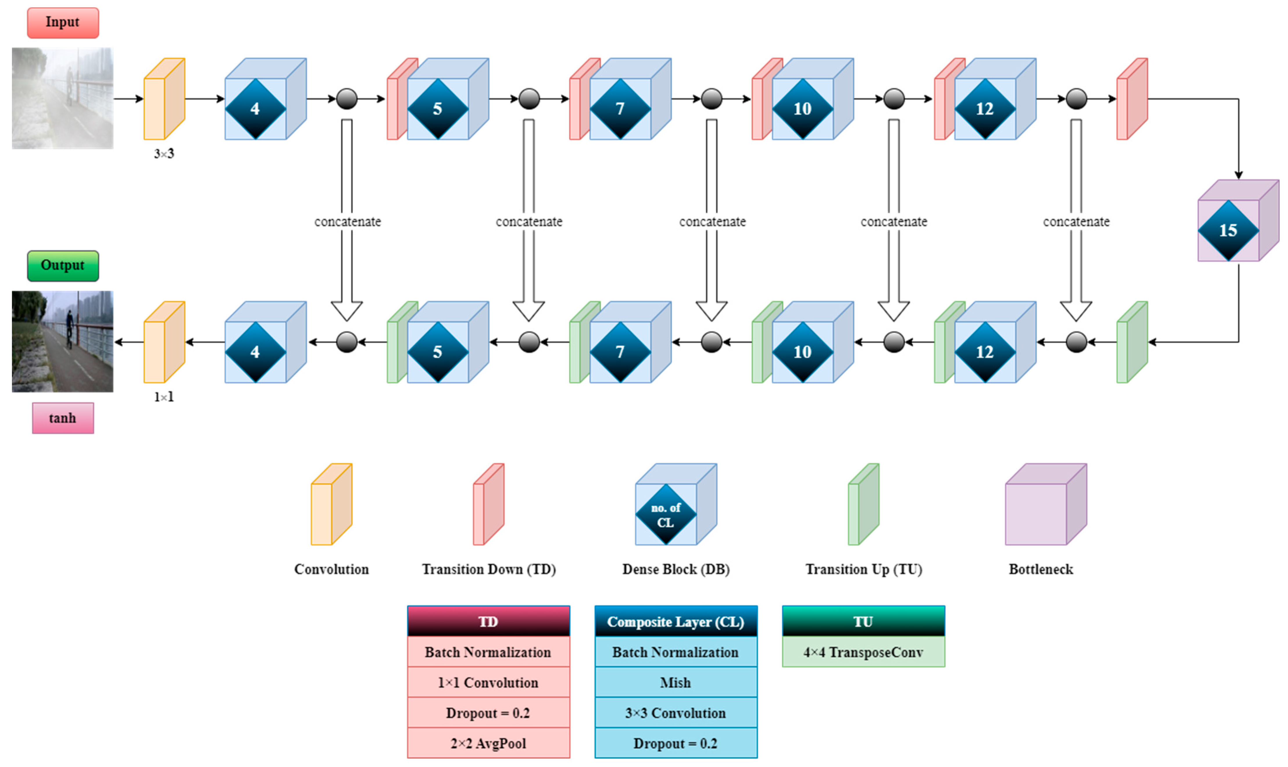
3.1. Generator Network

In the base model Dehaze-GAN, each dense block (DB) contains four composite layers (CLs). The activation function is ReLU. Figure 2 shows the generator network (G) of our proposed image dehazing model. There are five DBs in the encoder and five DBs in the decoder. On the encoder side, each DB is followed by a down-sampling layer. Similarly, on the decoder side, each DB is followed by an up-sampling layer. The decoder can generate a high-resolution image due to the concatenation of detailed features from the encoder side. We substantially extended the generator network from the base model of 56 layers to 103 layers. In deep learning, more layers do not imply better results and accuracy. The performance of the model depends on various factors such as the number of training samples, regularization technique, etc. For instance, a complex network trained with insufficient data may lead to overfitting. Oppositely, a shallow network may suffer from the underfitting problem when it is trained with a large amount of data. Through thorough experimentation, and as demonstrated in our superior results, we designed G with 103 layers.

We proposed G which differs from the base model with two modifications. First, in contrast with the base model, which contained a constant number of CLs in each DB, our generator network has progressively more CLs in the encoder. The number shown in each DB in Figure 2 is the number of CLs. This structure, with more non-linear computational power towards the end of the encoder, can capture the transformations at the multiple scales needed for artifact removal. In general, more layers in a network means more features can be extracted from the raw data. This can lead to better accuracy, provided that the training dataset is large enough. If the network contains more layers than necessary for the application, those unnecessary layers may try to extract some useless/unrelated features. This problem of overfitting will produce erroneous results. Second, we adopted Mish f(x) as the activation function. Mish is a state-of-the-art activation function [37]. It is a composite function of two existing activation functions, tanh and softplus.

$$f\left(x\right)=x\times tanh\left(softplus\left(x\right)\right)$$

(1)

$$softplus\left(x\right)=ln(1+e^x)$$

(2)

Mish has superior performance over other activation functions such as Swish and ReLU. It allows a better gradient flow than ReLU due to the slight allowance for negative values. Instead of a hard zero bound in ReLU, a smoother activation function can also enhance the backpropagation process, which allows more information to flow into the neural network deeply and, thus, leads to a better accuracy and generalization. A drawback of using Mish is the slight increase of network complexity, which leads to a longer training time. However, considering the higher accuracy and better training stability that Mish can accomplish, it was well worth adopting it in our proposed model. We demonstrate the superiority of our proposed generator network with one example of the progression of the generator output in Figure 3. Our proposed generator network could eventually produce an output which resembled the clear image.

3.2. Discriminator

Figure 4 shows the discriminator of our proposed image dehazing model. It consists of four layers of strided convolution. The inputs were the hazy image concatenated with the clear image and the generated fake image. The activation function at the output layer was sigmoid. The discriminator performed a patch-wise comparison of the clear image with the generated fake image to determine whether the generator output was real or fake. Therefore, the discriminator forced the generator to improve the realness of the output and helped remove the artifacts in the hazy image. In our experimentation, we had two versions of discriminator. The first one (D1) was the same as the base model with the use of LeakyReLU as the activation function. The second one (D2) utilized Mish as the activation function.

3.3. Loss Function and Training

The G and D of the image dehazing model were trained simultaneously, where G minimized the generative objective, and D maximized the discriminator objective. Therefore, the training process was formulated as a min–max of loss function. The generator objective L_G consisted of three weighted terms—standard objective L_gan, L₁ loss and perceptual loss L_p.

$$L_G=W_{gan}{L}_{gan}+W_{L1}{L}_{L1}+W_p{L}_p$$

(3)

$$L_{gan}=-mean\left[\mathit{log}\left(D\left(x,G\left(x\right)\right)\right)\right]$$

(4)

$$L_{L1}=E_{x,y}\left[{‖y^{\prime }-G\left(x\right)‖}_1\right]$$

(5)

$$L_p=c\times mse\left[V\right(G\left(x\right),V\left(y^{\prime }\right)\left)\right]$$

(6)

where x is the hazy image, y′ is the clear image, V is the VGG-19 network and W_gan, W_L1 and W_p are the weights to be determined empirically. L_p is the mean squared error (mse) between the VGG-19 outputs of the dehazed image and clear image scaled by the constant c. The discriminator objective is as follows:

$$L_D=mean\left[\mathit{log}\left(D\left(y^{\prime },y\right)\right)+log(1-D\left(x,G\left(x\right)\right))\right]$$

(7)

The model was trained on a computer with Intel Xeon Silver 4108 16-core CPU, Nvidia RTX 2080Ti GPU, and 55 GB RAM. In our experimentations, the dataset was partitioned into around 90% training samples and 10% testing samples. To find the best set of hyperparameters, 20% of the training samples were selected as a validation set. The model was trained with a learning rate of 0.001. The training process stopped when there was no improvement in accuracy.

4. Target Detection

Object detection is the foremost process in many image-based applications. It aims to detect the RoIs of the target objects in the image. A one-stage detector conducts target positioning and classification in the last convolutional layer in one pass. It has a faster operating speed with lower accuracy. For instance, You Only Look Once (YOLO) [28] is a powerful and widely used one-stage object detector. We select YOLO v5s, which is one of the latest versions, as the object detector. The model was the best choice in terms of balancing the requirements of detection accuracy and detection speed in road scene images.

The YOLO model first resizes the input image to a square matrix and partitions it into a number of grid cells. The network contains 24 convolutional layers and 2 fully connected layers. The function of these convolutional layers is to perform feature extraction. Fully connected layers are to generate the position and confidence score of detected objects. Each grid cell will respond to the detected class of object with the predicted bounding box and confidence score. The prediction consists of five values—the x-coordinate, y-coordinate, width and height of the bounding box and confidence score. The x- and y-coordinates are at the center of the box. The width and height are the distance between the boundary and the center of the bounding box. The confidence score represents the probability that the specific object is in the bounding box. The class-specific confidence score is calculated based on the appearance and positional information. Final results are generated after non-maximum suppression (NMS) in order to discard the duplicated detections.

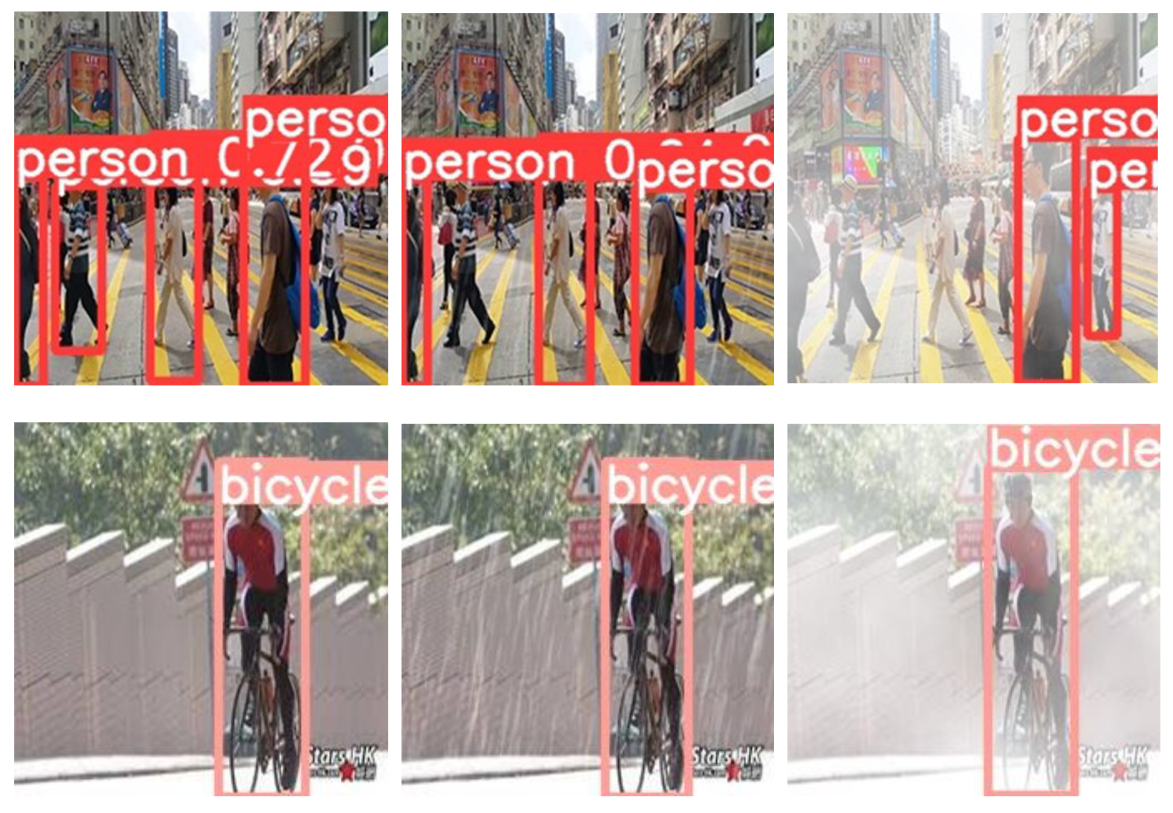
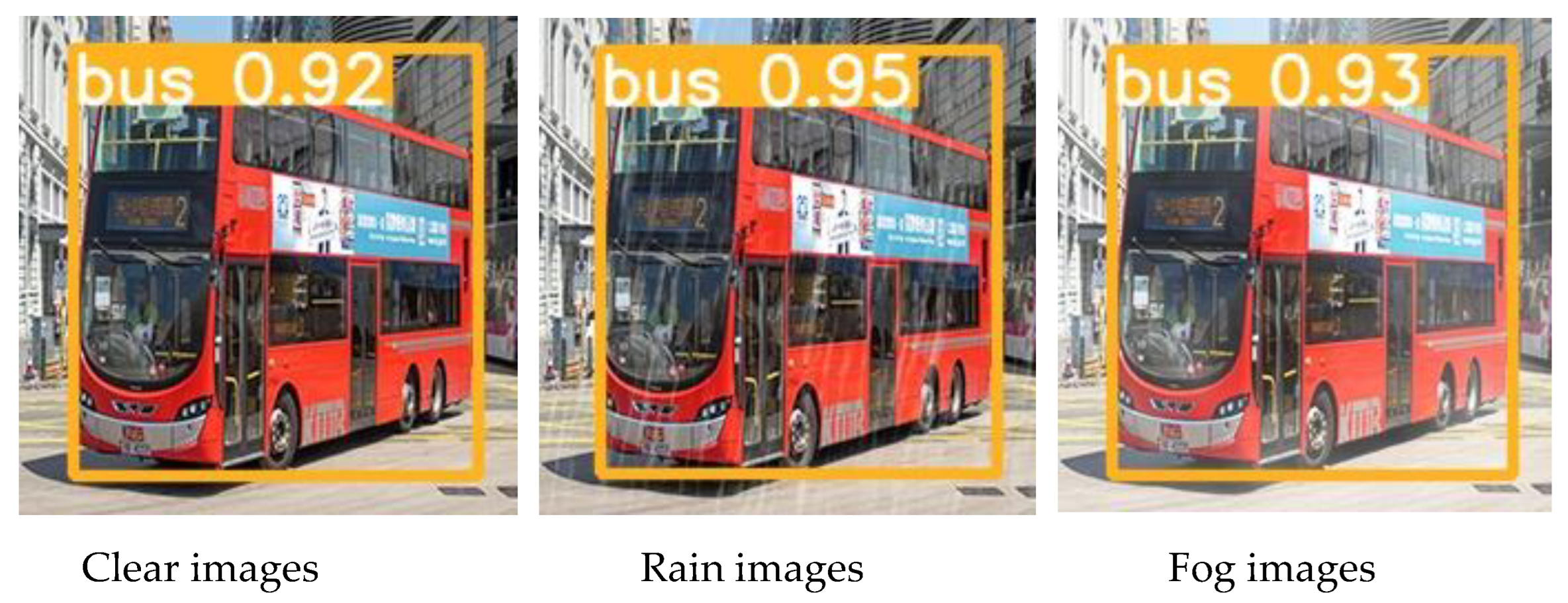
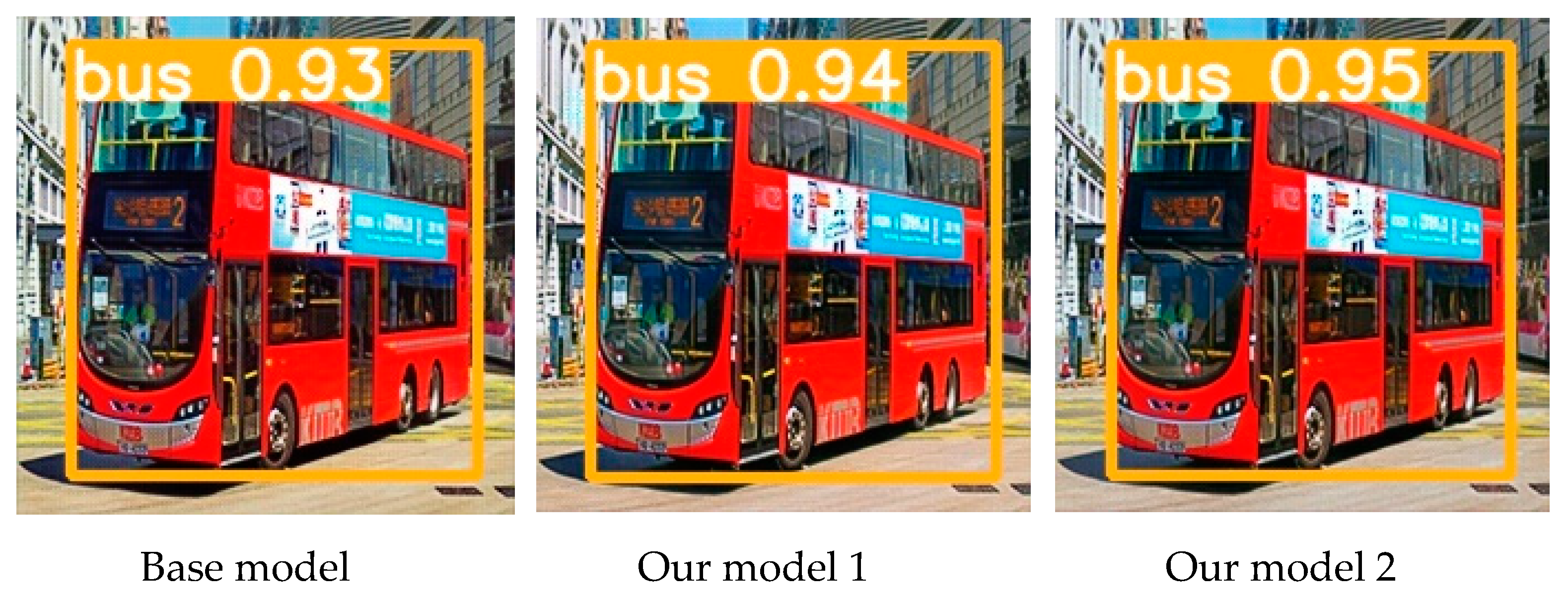
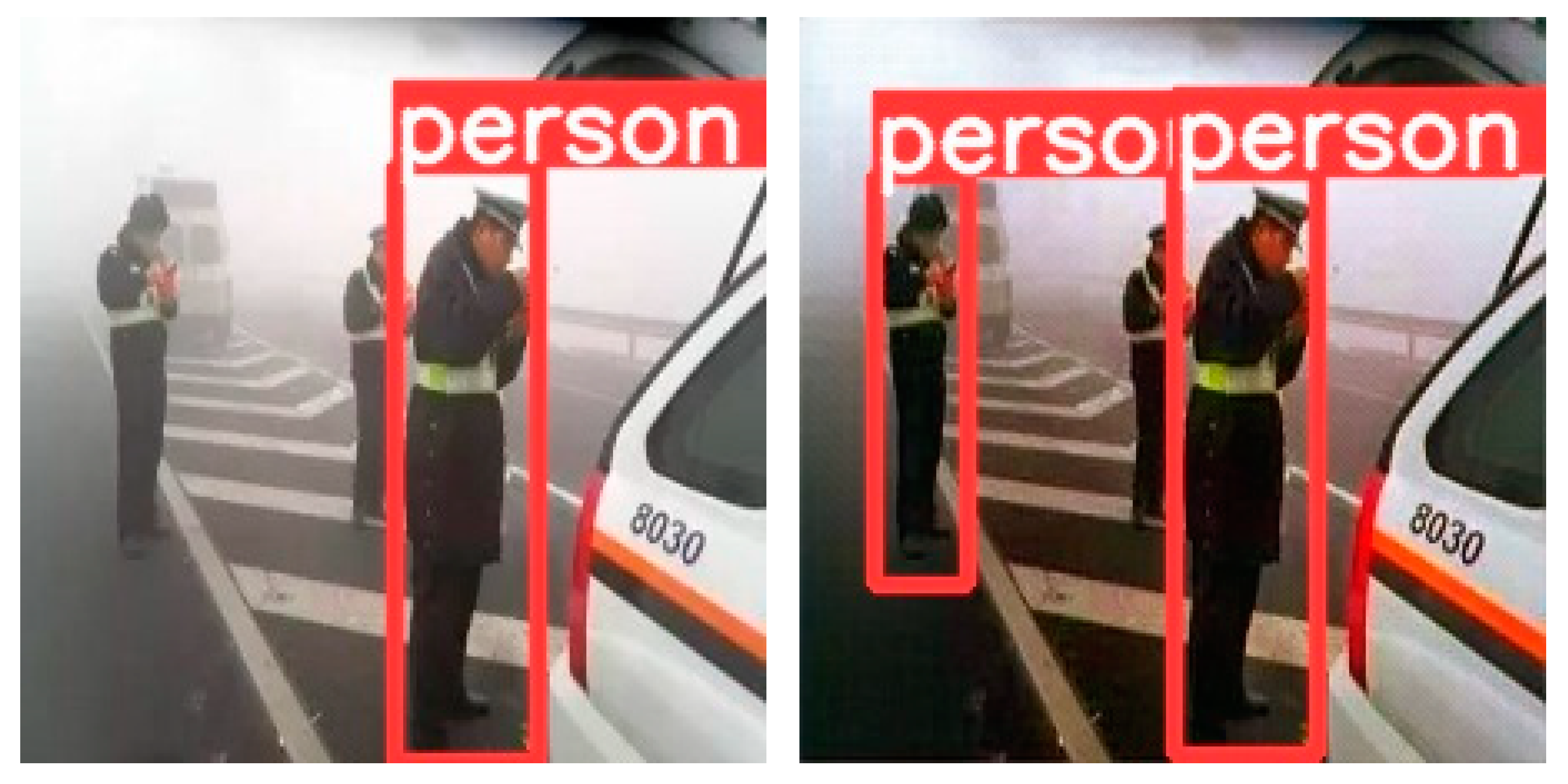
We observed that images degraded by rain and fog produce target object predictions with lower accuracy than those obtained from clear images. Therefore, in this experimentation, we investigated the significance of using dehazed images for road scene target detection. The results of target detection, as presented in Section 5, were obtained from clear images, degraded images and dehazed images. We illustrate the improvement of target detection in dehazed images over degraded images in terms of the dimension and confidence score of the detected targets.

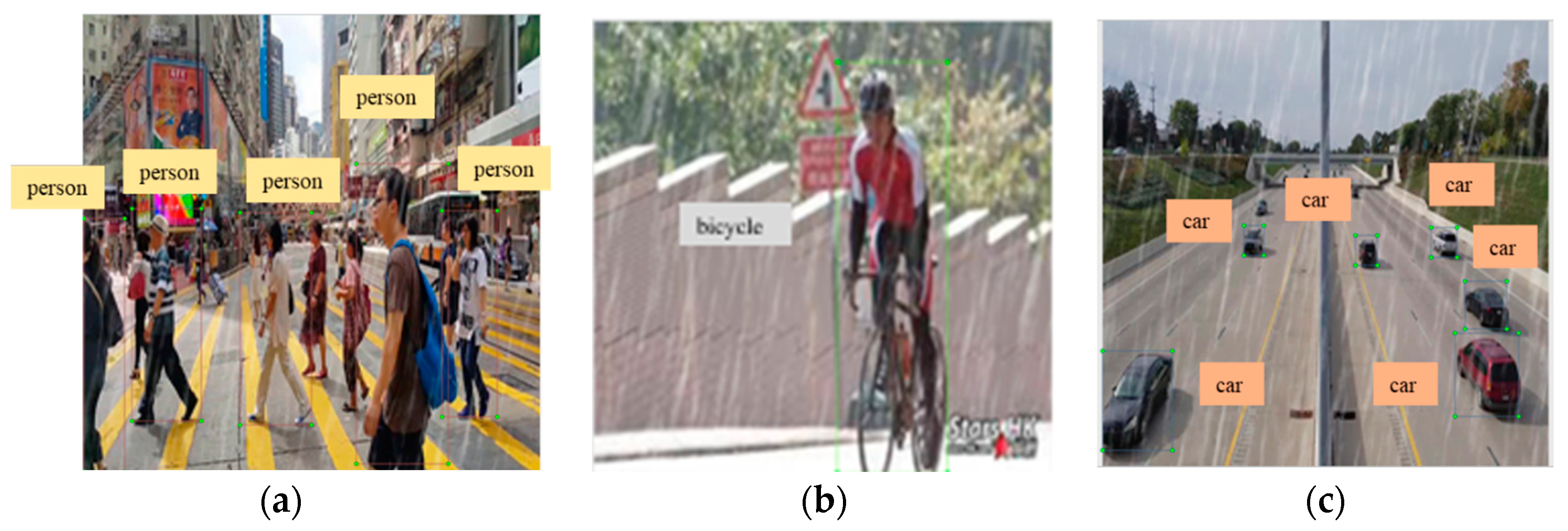
It is necessary to train the object detector with custom image samples rather than using a pre-trained model. We created the first dataset with 5509 road scene images collected online. Five target objects, as shown in

Table 1. Annotated targets and their quantities.

Type of Target	Number of Annotations
Pedestrian	1150
Bicycle	2100
Car	2050
Bus	1900
Truck	1950

, were annotated. Figure 5 shows some image samples with annotated targets. The images are of good visibility and were considered clear image samples.

We then created two degraded image datasets. Clear images were degraded with two weather conditions (rain and fog). Acquiring real images under raining and foggy weather conditions at the same location and the same time of the day as the clear images would be extremely difficult. Therefore, we adopted the approach of synthesizing and adding the weather conditions to the clear image.

Table 2. Synthesis of image degraded with rain.

Rain Synthesis
Create a blank background layer
Add Gaussian noise
Add Gaussian blur and motion blur
Add ripple distortion and Gaussian blur
Adjust intensity of background layer
Merge background layer with original image

shows the steps of the synthesis of rain. Figure 6 shows some images degraded with rain. Compared with the corresponding clear images, degraded images exhibited long thin white lines simulating the heavy rain. Fog was synthesized by adding two cloud layers with different fill opacities to the clear image.

Table 3. Synthesis of image degraded with fog.

Fog Synthesis
Duplicate the original image as background layer
Set the blending effect as soft light
Add render filter with different clouds
Fill the clouds with white
Duplicate the clouds layer
Transform first cloud layer by x: −8.61 cm y: −12.03cm
Transform second cloud layer by x: +4.69 cm y: −10.51cm
Set the fill opacity to 75% for first cloud layer and 50% for second cloud layer

shows the steps and parameter settings for the synthesis of fog. Figure 7 shows some images degraded with fog. The degraded images are covered with dense fog.

Finally, we created two dehazed datasets from the rain and fog degraded images. Dehazed images were generated using the image dehazing method as described in the Section 3. Five object detection models (clear, rain, fog, dehazed rain, and dehazed fog) were trained with supervised learning. The models were trained on a computer with AMD R7 3700X CPU, Nvidia RTX 2070s GPU, 16 GB RAM and 2 TB disk memory. Each dataset was partitioned into an 80% training sample and 20% validation sample. Each model was trained with the Adam optimizer and a learning rate of 0.001. The training process stopped when there was no improvement in the last 100 epochs. To find the best set of hyperparameters, we adopted five-fold validation.

5. Experiments and Results

The source code and the datasets used in the paper are publicly available at the following website: https://github.com/tychow45/cGAN_YOLOv5 (accessed on 20 April 2023).

5.1. Image Dehazing Result

In the first experiment, the performance of the proposed image dehazing model was evaluated and compared with other methods using two datasets. The first dataset was a combination of NYU-Depth V2 [38] and RESIDE-β [39]. NYU-Depth V2 contains indoor scenes with synthetic heavy haze, while RESIDE-β contains outdoor scenes with synthetic light haze. There were 2800 images in total (1424 from NYU-Depth V2 and 1376 from RESIDE-β). A total of 2500 images were taken as the training set. The remaining 300 images were used as the test set. To further evaluate the performance of our model on outdoor images, we also utilized the Synthetic Objective Testing Set (SOTS) which is a subset of RESIDE. It contains 500 pairs of real outdoor images with and without synthetic haze.

We adopted three evaluation metrics—the peak signal-to-noise ratio (PSNR), structural similarity index measure (SSIM) and a score which was a weighted sum of the PSNR and SSIM:

$$Score=W_{PSNR}\times PSNR+W_{SSIM}SSIM$$

(8)

where W_PSNR and W_SSIM were set to 0.05 and 1, respectively.

Table 4. Results of image dehazing on NYU/RESIDE dataset.

Method	PSNR	SSIM	Score
DCP [8]	17.23	0.803	1.665
BCCR [40]	15.12	0.719	1.475
AOD-Net [14]	11.63	0.624	1.206
Base model [36]	23.18	0.845	2.004
Our model	25.14	0.876	2.133

shows the results of our proposed model and four other methods on the NYU/RESIDE dataset. The base model performed better than the methods that utilized hand-crafted features (DCP, BCCR [40]) and the deep learning-based method (AOD-Net). Our proposed model achieved a further improvement in accuracy (nearly an increment of 2dB in PSNR over the base model) and outperformed all other methods.

Table 5. Results of image dehazing on SOTS dataset.

Method	PSNR	SSIM	Score
DCP [8]	18.66	0.873	1.806
BCCR [40]	14.02	0.757	1.458
AOD-Net [14]	18.48	0.833	1.757
Base model [36]	22.24	0.891	2.003
Our model	22.91	0.901	2.046

shows the results with the SOTS dataset. Again, our proposed model outperformed all other methods in terms of all evaluation metrics. The improvements over the base model were due to the changes to the cGAN structure and the activation function. Our proposed model could learn better from the training samples with the additional computation layers for feature extraction. Moreover, the training was more effective with the new activation function that could provide better gradient flow.

Table 6. Inference time per image.

Method	Inference Time (s)
Base model [36]	0.029
Our model	0.044

compares the inference time per image between our proposed model and the base model. Since our image dehazing model contained more computation layers than the base model, it demanded a longer inference time. Our model was still able to generate the dehazed image in near real-time speed.

The score parameter was ranked as medium, good or excellent. A score of 1.7 was considered medium (i.e., PSNR = 20 dB, SSIM = 0.7). A score of 2.0 was considered good (i.e., PSNR = 24 dB, SSIM = 0.8). A score of 2.5 was considered excellent (i.e., PSNR = 30 dB, SSIM = 1). According to this ranking scheme, the DCP and AOD-Net were between medium to good, and the base model was good. Our proposed model, as shown from the results on NYU/RESIDE and SOTS datasets in Table 4 and Table 5, Table 4 was ranked between good and excellent.

Figure 8 shows some visual results (indoor and outdoor images) on the NYU/RESIDE dataset. The methods that employ hand-crafted features produced darker images with distorted colors. AOD-Net produced more natural airlight in the outdoor scene, but the image was still dark. It was unable to remove the haze in the indoor image (it also had the worst numerical results in Table 3). The base model achieved better visual results. However, there were color distortions in some regions of the outdoor image, and the restored indoor image was blurred. Our model generated very natural colors in the outdoor image. The sky and trees were almost the same as those in the clear image. Our model also generated a much clearer indoor image than the base model (see the bookshelves). Figure 9 shows some visual results using the SOTS dataset. DCP and BCCR both had the same problem of color distortion. The dehazed images were dark. The base model performed better than AOD-Net, but the sky did not look natural and some haze was not removed. Our proposed model produced high quality haze removal. As compared with the results of the base model, our proposed model generated dehazed images with no color distortions in the sky. The buildings were very similar to those in the clear images.

In the previous experiment, we demonstrated that the framework of cGAN outperformed various hand-crafted and deep learning-based methods with image dehazing datasets. In the second experiment, we aimed to evaluate some cGAN models in order to select the best model. We compared two versions of our cGAN model with the base model on custom datasets of road scene images.

Table 7. Results of image dehazing on rain dataset.

Method	PSNR	SSIM	Score
Base model [36]	29.43	0.937	2.408
Our model 1 (G + D1)	30.02	0.944	2.445
Our model 2 (G + D2)	30.05	0.948	2.451

shows the results using the rain dataset.

Table 8. Results of image dehazing on fog dataset.

Method	PSNR	SSIM	Score	VCM	CNI	FRF
Base model [36]	22.40	0.885	2.005	48.66	0.56	1.94
FFA-Net [18]	18.26	0.836	1.749	55.51	0.49	1.47
MSBDN [20]	19.01	0.876	1.827	55.00	0.53	1.65
Our model 1 (G + D1)	22.47	0.890	2.014	51.69	0.61	1.88
Our model 2 (G + D2)	23.16	0.896	2.054	50.04	0.59	1.92

shows the results using the fog dataset with three more evaluation parameters: the visual contrast measure (VCM), color naturalness index (CNI) and fog reduction factor (FRF) [41]. Fog is a more serious defect than rain. In general, the evaluation metrics obtained on the fog dataset were lower than those of the rain dataset. We also compared our proposed models with two state-of-the-art image dehazing methods: FFA-Net [18] and MSBDN [20]. Figure 10 shows some visual results obtained using our proposed model 2, FFA-Net and MSBDN. With the two modifications in our design, both versions of our cGAN model achieved better performance than the base model (more than 0.6 dB in PSNR with the rain dataset and more than 0.7 dB in PSNR with the fog dataset). Furthermore, with the adoption of Mish as the activation function in the discriminator, model 2 could further improve the dehazing as compared with model 1.

Furthermore, we performed an additional image dehazing experiment using the Real-world Task-driven Testing Set (RTTS) in the RESIDE dataset which contains real and strong hazy images. Figure 11 shows some visual results obtained using the base model and our proposed model 2. The visual results demonstrated that the dehazed images generated using our proposed model could restore the details of the buildings and the colors of the sky better than the base model (see the red boxes highlighted in the images).

5.2. Object Detection Result

To investigate the significance of image dehazing on object detection, we compared the accuracy of target detection using two versions of our cGAN model with the base model. We created five datasets of road scene images—clear images, rain images, fog images, dehazed rain images and dehazed fog images.

Table 9. Object detection accuracy with clear images, rain images and fog images.

Category	Clear Image		Rain Image		Fog Image
	mAP @0.5	mAP @0.95	mAP @0.5	mAP @0.95	mAP @0.5	mAP @0.95
Pedestrian	0.782	0.455	0.740	0.425	0.730	0.415
Bicycle	0.871	0.651	0.858	0.635	0.842	0.622
Car	0.954	0.675	0.952	0.678	0.937	0.664
Bus	0.976	0.850	0.979	0.856	0.974	0.865
Truck	0.966	0.807	0.963	0.805	0.854	0.811
All	0.910	0.688	0.898	0.680	0.886	0.675

shows the object detection accuracy mAP on clear images, rain images and fog images. The rain and fog images were generated with the weather effects synthesized and overlayed on the clear images. No image dehazing was performed on the rain and fog images. It was clear that using degraded images would lead to lower object detection accuracy in all object classes. The overall mAP on rain images and fog images dropped by 0.012 and 0.024, respectively, as compared with the corresponding result with clear images. In some categories, the reduction in accuracy was more substantial. For instance, in the class of pedestrian, the mAP on rain images and fog images reduced by 0.042 and 0.052, respectively, as compared with the corresponding result for clear images.

Table 10. Object detection accuracy with dehazed rain images.

Category	Base Model [36]		Our Model 1 (G + D1)		Our Model 2 (G + D2)
	[email protected]	[email protected]	[email protected]	[email protected]	[email protected]	[email protected]
Pedestrian	0.766	0.444	0.821	0.459	0.777	0.462
Bicycle	0.865	0.644	0.868	0.658	0.868	0.631
Car	0.957	0.680	0.966	0.674	0.956	0.678
Bus	0.969	0.849	0.966	0.838	0.974	0.856
Truck	0.958	0.796	0.929	0.796	0.956	0.802
All	0.903	0.683	0.910	0.685	0.906	0.686

compares two versions of our cGAN model with the base model using dehazed rain images. The utilization of the cGAN framework for image dehazing could significantly improve the object detection accuracy. Our proposed models achieved a further gain in accuracy in some object classes (e.g., pedestrian, bicycle, car) and also the highest overall accuracy.

Table 11. Object detection accuracy mAP @0.5 with dehazed fog images.

Category	Base Model [36]	FFA-Net [18]	MSBDN [20]	Our Model 1 (G + D1)	Our Model 2 (G + D2)
Pedestrian	0.765	0.849	0.923	0.786	0.774
Bicycle	0.864	0.885	0.944	0.866	0.870
Car	0.957	0.942	0.973	0.954	0.955
Bus	0.966	0.966	0.983	0.964	0.967
Truck	0.955	0.952	0.977	0.949	0.950
All	0.902	0.919	0.960	0.903	0.903

compares two versions of our cGAN model with the base model, FFA-Net [18], and MSBDN [20] using dehazed fog images. Although fog is a more serious defect than rain, the object detection accuracy on the dehazed fog dataset was close to that obtained with the dehazed rain dataset. This demonstrates the effectiveness of the cGAN framework in tackling different types of degradation. Our proposed models achieved better performance than the base model in some object classes (e.g., pedestrian, bicycle, bus), and also the highest overall accuracy. Our proposed model 2 also achieved better performance than FFA-Net in the object classes of car and bus. The confidence score was a numeric result (between 0 to 1) produced by the object detector. It represents the likelihood of the recognized class of object.

Table 12. Average confidence score.

Method	Rain Image	Fog Image
No image dehazing	0.791	0.753
Base model [36]	0.804	0.802
Our model 1 (G + D1)	0.803	0.801
Our model 2 (G + D2)	0.804	0.802

compares the average confidence scores of degraded images and dehazed images. cGAN improved the confidence score of the dehazed rain image and fog image by 0.013 and 0.049, respectively, over the degraded images. This further illustrated the benefit of dehazed images over degraded images in object detection, in particular with regard to foggy images.

Figure 12 shows the visual results of object detection with clear images, rain images and fog images. Target objects, e.g., pedestrians and cars, may have been missed in degraded images. Figure 13 shows the corresponding visual results with dehazed rain images. While some objects were not detected in the degraded images, they were detected in the dehazed images. In comparison with the base model, our proposed models could better predict the bounding boxes (see the blue circles highlighted in the pedestrian and bus images) and achieved higher confidence scores (e.g., bus). Figure 14 shows the corresponding visual results with dehazed fog images. In comparison with the base model, our models removed the fog more effectively (see the bicycle images). Our model 1 better predicted the bounding boxes (e.g., pedestrian). Our model 2 achieved high confidence scores that were close to or higher than those achieved with the base model.

Furthermore, we performed an additional object detection experiment on the RTTS dataset. We did not re-train our proposed model 2 for this dataset.

Table 13. Object detection accuracy with RTTS.

Category	# Labels	Original Hazy Images		Dehazed Image by Model 2
		mAP @0.5	mAP @0.95	mAP @0.5	mAP @0.95
Pedestrian	2447	0.622	0.337	0.570	0.303
Bicycle	338	0.617	0.418	0.664	0.443
Car	4430	0.595	0.413	0.602	0.422
Bus	6	0.039	0.031	0.035	0.029
Truck	127	0.066	0.047	0.083	0.057
All	7348	0.388	0.249	0.391	0.251

shows a comparison of the accuracy of object detection with the original hazy images and dehazed images generated using our proposed model 2. Figure 15 shows some visual results obtained with the original hazy images and the dehazed images generated using our proposed model 2. The numerical and visual results demonstrated that the dehazed images generated using our proposed model could result in better object detection than the original hazy images.

6. Conclusions

We designed a novel single end-to-end network based on the cGAN framework for image dehazing. We strengthened the analytical power of the network via the adoption of convolutional blocks with progressively more layers. Moreover, the entire dehazing framework was enhanced with the adoption of a new non-linear activation function in both the generator and discriminator modules. The dehazed image was beneficial for the detection of objects in degraded road scene images. Based on the enhanced framework, we proposed two image dehazing models with two discriminators. Through thorough experimentation, we demonstrated that our proposed image dehazing models improved the visibility of the degraded images and resulted in a higher accuracy of object detection. Our proposed models outperformed not only the hand-crafted and deep learning-based methods, but also the cGAN base model using various datasets.

We will continue our research on image dehazing. In the current work, we investigated the impact of our proposed image dehazing model on object detection performed on images degraded with rain and fog effects. More experimentation will be performed to investigate the capability of our proposed model in tackling other types of image degradation. Besides object detection in 2D images, we will also explore the impact of image dehazing on other applications such as monocular 3D object detection.

For practical applications, we will consider integrating the image dehazing as an optional module within the object detection framework. To save computational costs, there is no need to perform image dehazing when the scene visibility is good. Automatically triggering the execution of the image dehazing module is possible via computation of the similarity between the hazy input image and the dehazed output image. Significant changes in quantitative measures, e.g., SSIM, will enable the continuing function of the image dehazing module. An automatic alert of extreme conditions would be possible when the confidence score of an object detection is low.

References

1. Gao, M.; Wang, J.; Chen, Y.; Du, C.; Chen, C.; Zeng, Y. An improved multi-exposure image fusion method for intelligent transportation system. Electronics 2021, 10, 383. [Google Scholar] [CrossRef]
2. Liu, X.; Zhao, C.; Zhang, Q.; Yang, C.; Zhang, J. Characterizing and monitoring ground settlement of marine reclamation land of Xiamen New Airport, China with Sentinel-1 SAR datasets. Remote Sens. 2019, 11, 585. [Google Scholar] [CrossRef]
3. Tarel, J.-P.; Hautière, N.; Cord, A.; Gruyer, D.; Halmaoui, H. Improved visibility of road scene images under heterogeneous fog. In Proceedings of the IEEE Intelligent Vehicles Symposium 2010, La Jolla, CA, USA, 21–24 June 2010; pp. 478–485. [Google Scholar]
4. Jia, Z.; Wang, H.C.; Caballero, R.E.; Xiong, Z.Y.; Zhao, J.W.; Finn, A. A two-step approach to see-through bad weather for surveillance video quality enhancement. Mach. Vis. Appl. 2012, 23, 1059–1082. [Google Scholar] [CrossRef]
5. Pan, X.X.; Xie, F.Y.; Jiang, Z.G.; Yin, J.H. Haze removal for a single remote sensing image based on deformed haze imaging model. IEEE Signal Process. Lett. 2015, 22, 1806–1810. [Google Scholar] [CrossRef]
6. Babu, G.H.; Venkatram, N. A survey on analysis and implementation of state-of-the-art haze removal techniques. J. Vis. Commun. Image Represent. 2020, 72, 102912. [Google Scholar] [CrossRef]
7. Wang, W.; Yuan, X. Recent advances in image dehazing. IEEE/CAA J. Autom. Sin. 2017, 4, 410–436. [Google Scholar] [CrossRef]
8. He, K.; Sun, J.; Tang, X. Single image haze removal using dark channel prior. In Proceedings of the IEEE Conference on Computer Vision and Pattern Recognition 2009, Miami, FL, USA, 20–25 June 2009; pp. 1956–1963. [Google Scholar]
9. Dharejo, F.A.; Zhou, Y.; Deeba, F.; Du, Y. A color enhancement scene estimation approach for single image haze removal. IEEE Geosci. Remote Sens. Lett. 2020, 17, 1613–1617. [Google Scholar] [CrossRef]
10. Galdran, A. Image dehazing by artificial multiple-exposure image fusion. Signal Process. 2018, 149, 135–147. [Google Scholar] [CrossRef]
11. Kumar, A.; Jha, R.K.; Nishchal, N.K. An improved gamma correction model for image dehazing in a multi-exposure fusion framework. J. Vis. Commun. Image Represent. 2021, 78, 103122. [Google Scholar] [CrossRef]
12. Chaudhry, A.M.; Riaz, M.M.; Ghafoor, A. A framework for outdoor RGB image enhancement and dehazing. IEEE Geosci. Remote Sens. Lett. 2018, 15, 932–936. [Google Scholar] [CrossRef]
13. Khaldi, B.; Aiadi, O.; Kherfi, M.L. Combining colour and grey-level co-occurrence matrix features: A comparative study. IET Image Process. 2019, 13, 1401–1410. [Google Scholar] [CrossRef]
14. Li, B.; Peng, X.; Wang, Z.; Xu, J.; Feng, D. AOD-Net: All-in-One Dehazing Network. In Proceedings of the International Conference on Computer Vision 2017, Venice, Italy, 22–29 October 2017; pp. 4780–4788. [Google Scholar]
15. Zhang, H.; Patel, V.M. Densely connected pyramid dehazing network. In Proceedings of the IEEE/CVF Conference on Computer Vision and Pattern Recognition 2018, Salt Lake City, UT, USA, 18–23 June 2018; pp. 3194–3203. [Google Scholar]
16. Dong, Y.; Liu, Y.; Zhang, H.; Chen, S.; Qiao, Y. FD-GAN: Generative adversarial networks with fusion-discriminator for single image dehazing. In Proceedings of the AAAI Conference on Artificial Intelligence 2020, New York, NY, USA, 7–12 February 2020; pp. 10729–10736. [Google Scholar]
17. Guo, C.; Yan, Q.; Anwar, S.; Cong, R.; Ren, W.; Li, C. Image dehazing transformer with transmission-aware 3D position embedding. In Proceedings of the IEEE/CVF Conference on Computer Vision and Pattern Recognition 2022, New Orleans, LA, USA, 18–24 June 2022; pp. 5812–5820. [Google Scholar]
18. Qin, X.; Wang, Z.; Bai, Y.; Xie, X.; Jia, H. FFA-Net: Feature fusion attention network for single image dehazing. In Proceedings of the AAAI Conference on Artificial Intelligence 2020, New York, NY, USA, 7–12 February 2020; pp. 11908–11915. [Google Scholar]
19. Wu, H.; Qu, Y.; Lin, S.; Zhou, J.; Qiao, R.; Zhang, Z.; Xie, Y.; Ma, L. Contrastive learning for compact single image dehazing. In Proceedings of the IEEE/CVF Conference on Computer Vision and Pattern Recognition 2021, Nashville, TN, USA, 20–25 June 2020; pp. 10551–10560. [Google Scholar]
20. Dong, H.; Pan, J.; Xiang, L.; Hu, Z.; Zhang, X.; Wang, F.; Yang, M.-H. Multi-scale boosted dehazing network with dense feature fusion. In Proceedings of the IEEE/CVF Conference on Computer Vision and Pattern Recognition 2020, Seattle, WA, USA, 13–19 June 2020; pp. 2157–2167. [Google Scholar]
21. Su, Y.Z.; Cui, Z.G.; He, C.; Li, A.H.; Wang, T.; Cheng, K. Prior guided conditional generative adversarial network for single image dehazing. Neurocomputing 2021, 423, 620–638. [Google Scholar] [CrossRef]
22. Kan, S.; Zhang, Y.; Zhang, F.; Cen, Y. A GAN-based input-size flexibility model for single image dehazing. Signal Process. Image Commun. 2022, 102, 116599. [Google Scholar] [CrossRef]
23. Li, R.; Pan, J.; Li, Z.; Tang, J. Single image dehazing via conditional generative adversarial network. In Proceedings of the IEEE/CVF Conference on Computer Vision and Pattern Recognition 2018, Salt Lake City, UT, USA, 18–23 June 2018; pp. 8202–8211. [Google Scholar]
24. Ancuti, C.O.; Ancuti, C.; Timofte, R.; Vleeschouwer, C.D. I-HAZE: A dehazing benchmark with real hazy and haze-free indoor images. Lect. Notes Comput. Sci. LNCS 2018, 11182, 620–631. [Google Scholar]
25. Tarel, J.-P.; Hautiere, N.; Caraffa, L.; Cord, A.; Halmaoui, H.; Gruyer, D. Vision enhancement in homogeneous and heterogeneous fog. IEEE Intell. Transp. Syst. Mag. 2012, 4, 6–20. [Google Scholar] [CrossRef]
26. Sakaridis, C.; Dai, D.; Van Gool, L. Semantic foggy scene understanding with synthetic data. Int. J. Comput. Vis. 2018, 126, 973–992. [Google Scholar] [CrossRef]
27. Zhao, S.; Zhang, L.; Huang, S.; Shen, Y.; Zhao, S. Dehazing evaluation: Real-world benchmark datasets, criteria, and baselines. IEEE Trans. Image Process. 2020, 29, 6947–6962. [Google Scholar] [CrossRef]
28. Redmon, J.; Divvala, S.; Girshick, R.; Farhadi, A. You Only Look Once: Unified real-time object detection. In Proceedings of the IEEE Conference on Computer Vision and Pattern Recognition 2016, Las Vegas, NV, USA, 27–30 June 2016; pp. 779–788. [Google Scholar]
29. Liu, W.; Anguelov, D.; Erhan, D.; Szegedy, C.; Reed, S.; Fu, C.-Y.; Berg, A.C. SSD: Single Shot MultiBox Detector. In Proceedings of the European Conference on Computer Vision 2016, Amsterdam, The Netherlands, 11–14 October 2016; pp. 21–37. [Google Scholar]
30. Girshick, R.; Donahue, J.; Darrell, T.; Malik, J. Rich feature hierarchies for accurate object detection and semantic segmentation. In Proceedings of the IEEE Conference on Computer Vision and Pattern Recognition 2014, Columbus, OH, USA, 23–28 June 2014. [Google Scholar]
31. Ren, S.; He, K.; Girshick, R.; Sun, J. Faster R-CNN: Towards real-time object detection with region proposal networks. In Proceedings of the Neural Information Processing Systems 2015, Montreal, QC, Canada, 7–12 December 2015. [Google Scholar]
32. He, K.; Gkioxari, G.; Dollár, P.; Girshick, R. Mask R-CNN. In Proceedings of the IEEE International Conference on Computer Vision 2017, Venice, Italy, 22–29 October 2017; pp. 2980–2988. [Google Scholar]
33. He, K.; Zhang, X.; Ren, S.; Sun, J. Deep residual learning for image recognition. In Proceedings of the IEEE Conference on Computer Vision and Pattern Recognition 2016, Las Vegas, NV, USA, 27–30 June 2016; pp. 770–778. [Google Scholar]
34. Chen, Y.; Li, W.; Sakaridis, C.; Dai, D.; Van Gool, L. Domain adaptive Faster R-CNN for object detection in the wild. In Proceedings of the IEEE/CVF Conference on Computer Vision and Pattern Recognition 2018, Salt Lake City, UT, USA, 18–23 June 2018; pp. 3339–3348. [Google Scholar]
35. Wang, W.; Cao, Y.; Zhang, J.; He, F.; Zha, Z.-J.; Wen, Y.; Tao, D. Exploring sequence feature alignment for domain adaptive detection transformers. In Proceedings of the ACM International Conference on Multimedia 2021, Virtual, 20–24 October 2021; pp. 1730–1738. [Google Scholar]
36. Raj, N.B.; Venketeswaran, N. Single image haze removal using a Generative Adversarial Network. In Proceedings of the International Conference on Wireless Communications Signal Processing and Networking 2020, Chennai, India, 4–6 August 2020; pp. 37–42. [Google Scholar]
37. Misra, D. Mish: A self regularized non-monotonic activation function. arXiv 2019, arXiv:1908.08681. [Google Scholar]
38. Silberman, N.; Hoiem, D.; Kohli, P.; Fergus, R. Indoor segmentation and support inference from RGBD images. In Proceedings of the European Conference on Computer Vision 2012, Florence, Italy, 7–13 October 2012; pp. 746–760. [Google Scholar]
39. Li, B.; Ren, W.; Fu, D.; Tao, D.; Feng, D. Benchmarking single-image dehazing and beyond. IEEE Trans. Image Process. 2019, 28, 492–505. [Google Scholar] [CrossRef] [PubMed]
40. Meng, G.; Wang, Y.; Duan, J.; Xiang, S.; Pan, C. Efficient image dehazing with boundary constraint and contextual regularization. In Proceedings of the IEEE International Conference on Computer Vision 2013, Sydney, Australia, 1–8 December 2013; pp. 617–624. [Google Scholar]
41. Kansal, I.; Kasana, S.S. Improved color attenuation prior based image de-fogging technique. Multimed. Tools Appl. 2020, 79, 12069–12091. [Google Scholar] [CrossRef]
Figure 1. Overview of our image dehazing model.
Applsci 13 05326 g001
Figure 2. Our proposed generator network.
Applsci 13 05326 g002
Figure 3. Progression of generator output—clear image and generated images at various stages of prediction.
Applsci 13 05326 g003
Figure 4. The discriminator.
Applsci 13 05326 g004
Figure 5. Clear image samples with annotations: (a) pedestrian, (b) bicycle, (c) car, (d) bus, (e) truck.
Applsci 13 05326 g005
Figure 6. Image samples degraded with rain: (a) pedestrian, (b) bicycle, (c) car, (d) bus, (e) truck.
Applsci 13 05326 g006aApplsci 13 05326 g006b
Figure 7. Image samples degraded with fog: (a) pedestrian, (b) bicycle, (c) car, (d) bus, (e) truck.
Applsci 13 05326 g007aApplsci 13 05326 g007b
Figure 8. Visual results using NYU/RESIDE dataset—first row: clear images; second row: hazy im-ages; third row: images dehazed using DCP; fourth row: images dehazed using AOD-Net; fifth row: image dehazed using base model; last row: images dehazed using our proposed model.
Applsci 13 05326 g008aApplsci 13 05326 g008b
Figure 9. Visual results using SOTS dataset—first row: clear images; second row: hazy images; third row: images dehazed using DCP; fourth row: images dehazed using AOD-Net; fifth row: images dehazed using base model; last row: images dehazed using our proposed model.
Applsci 13 05326 g009aApplsci 13 05326 g009b
Figure 10. Visual results with fog dataset (from left): clear image, dehazed image generated using FFA-Net, dehazed image generated using MSBDN, dehazed image generated using our proposed model 2.
Applsci 13 05326 g010
Figure 11. Visual results on RTTS in RESIDE dataset—left column: original hazy images; middle column: dehazed images generated using base model; right column: images dehazed using our proposed model 2.
Applsci 13 05326 g011
Figure 12. Object detection results—first row: pedestrian; second row: bicycle; third row: car; last row: bus; first column: clear images; second column: rain images; last column: fog images.
Applsci 13 05326 g012aApplsci 13 05326 g012b
Figure 13. Object detection results with dehazed rain images—first row: pedestrian; second row: bicycle; third row: car; last row: bus; first column: images dehazed using base model; second column: images dehazed using our proposed model 1; last column: images dehazed using our proposed model 2.
Applsci 13 05326 g013aApplsci 13 05326 g013b
Figure 14. Object detection results with dehazed fog images—first row: pedestrian; second row: bicycle; third row: car; last row: bus; first column: image dehazed using base model; second column: images dehazed using our proposed model 1; last column: image dehazed using our proposed model 2.
Applsci 13 05326 g014aApplsci 13 05326 g014b
Figure 15. Object detection results with RTTS—left column: original hazy images; right column: dehazed images generated using our proposed model 2.
Applsci 13 05326 g015aApplsci 13 05326 g015b