
Application of an Optimized PSO-BP Neural Network to the Assessment and Prediction of Underground Coal Mine Safety Risk Factors

Abstract
1. Introduction
2. Material and Methods
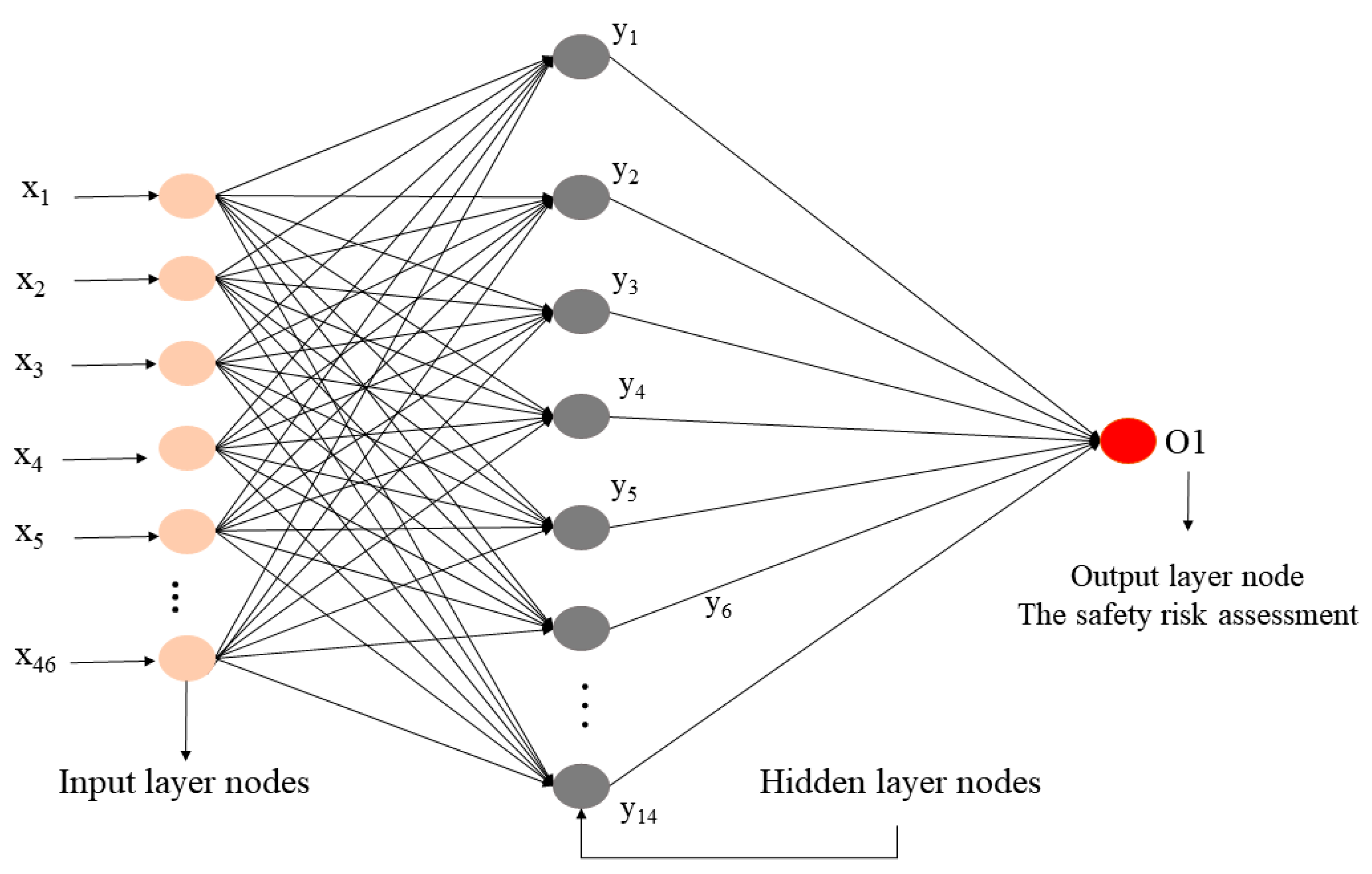
2.1. The BP Neural Network Model
- In feed-forward propagation in the BP neural network, the output of the hidden layer is described as follows:
- b.
- BP neural network Error
Simulation
- Activation function selection: The transfer function selection between the layers of the BP neural network is an important part of the network. The coal safety risk assessment depends on various factors, such as the problem’s complexity, the data set’s size, and the desired output. In this study, the hyperbolic tangent (tanh) and sigmoid functions were adopted for the hidden and output layers, respectively.
- Training function: The training function in the BP neural network is responsible for adjusting the network weights during the training process. The goal of the training function is to minimize the difference between the network’s output and the desired output for a given input. This study used the Levenberg–Marquardt algorithm as the best and optimal training function to adjust the connection weight and reduce the mean square error.
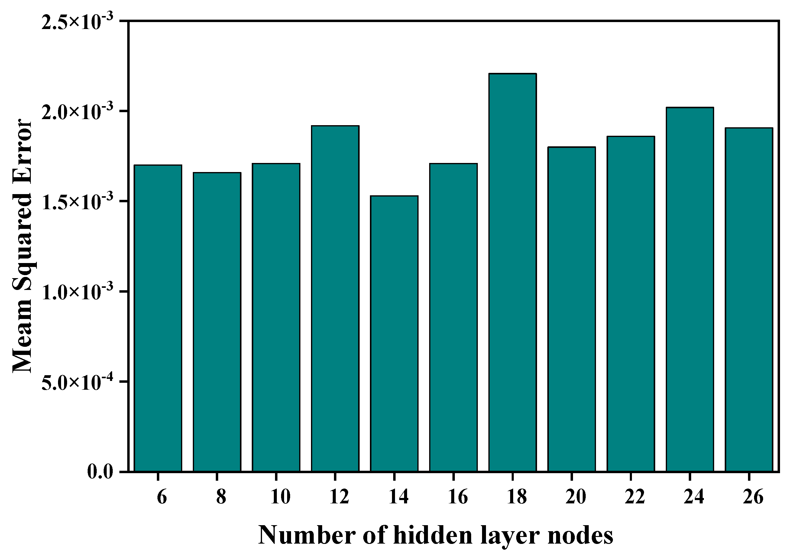
- Determination of the number of hidden layer nodes: the hidden layer node is determined based on the complexity of the problem being solved, the amount and quality of the available data, and the desired level of accuracy. Therefore, in this study, a trial-and-error approach was used. A different number of nodes was adopted, and the performances of the networks were compared. The performance was measured in terms of the mean square error (MSE). The number that performed best on the validation set was optimal, as shown in Figure 1.
- 4.
- Learning rate and lower momentum factor: The choice of the parameters in the BP neural network plays a critical role in the training process. A high learning rate can help the model converge quickly, but it may also cause the optimization algorithm to overshoot the optimal weight values and result in poor performance. A low learning rate, on the other hand, may cause the model to converge slowly or get stuck in local minima. The momentum factor can address these issues by helping the optimizer move more smoothly through the weight space and avoid getting stuck in local minima. A higher momentum factor can help the optimizer overcome local minima and reach the global minimum more quickly. In comparison, a lower momentum factor can help prevent overshooting and oscillations in the weight updates. In this study, to choose the best values for η and α, several BP neural network models were developed with η values of 0.02, 0.04, 0.06, 0.08, 0.01, and 0.2, respectively, and α values of 0.1, 0.2, 0.3, 0.4, 0.7, and 0.9, respectively. The MSE evaluation chose the optimal η and α values as 0.01 and 0.9, respectively.
2.2. Particle Swarm Optimization Algorithm
3. Network Optimization of the Coal Mine Safety Risk Assessment
3.1. Modeling
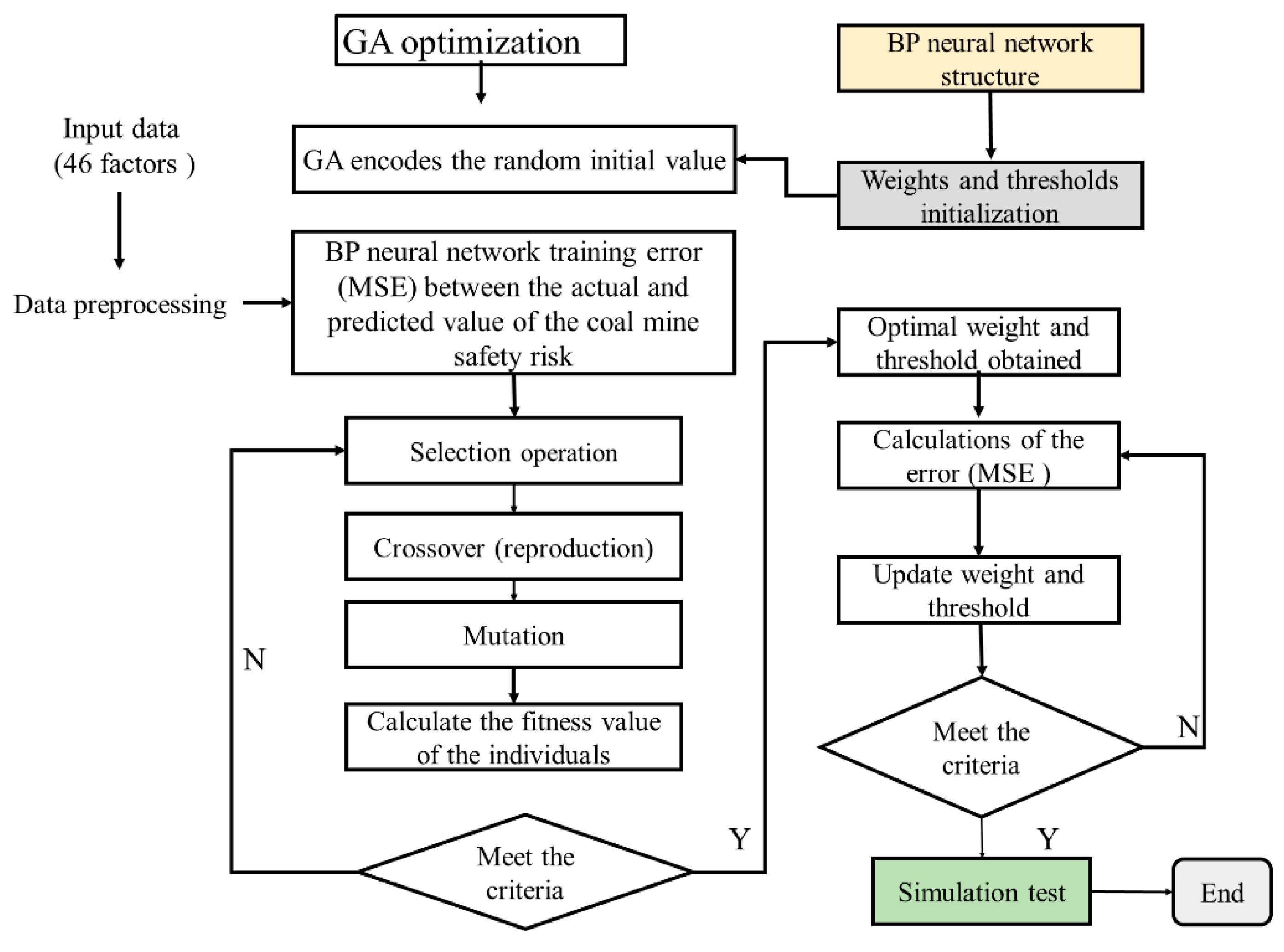
3.1.1. The GA-BP Neural Network
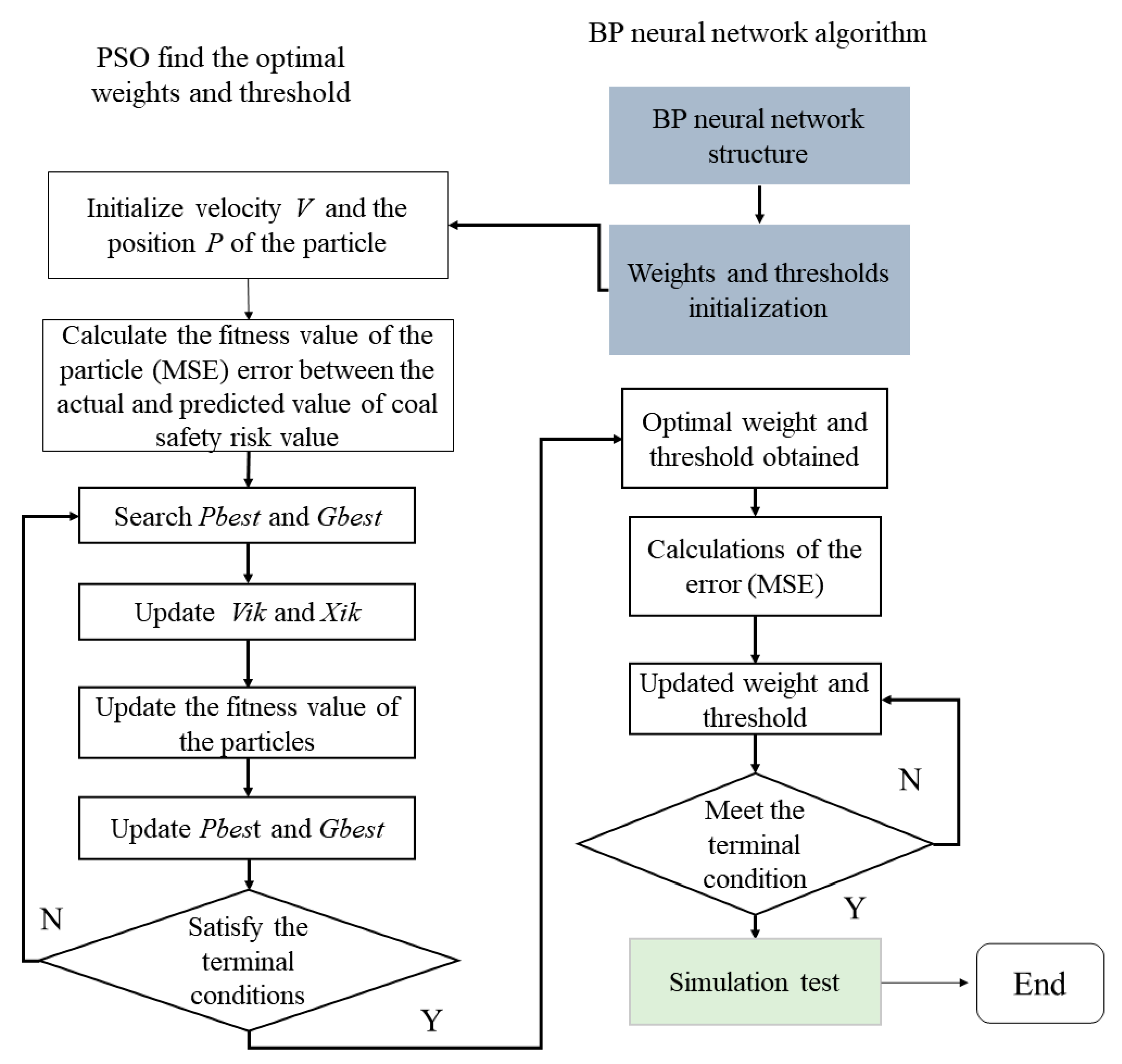
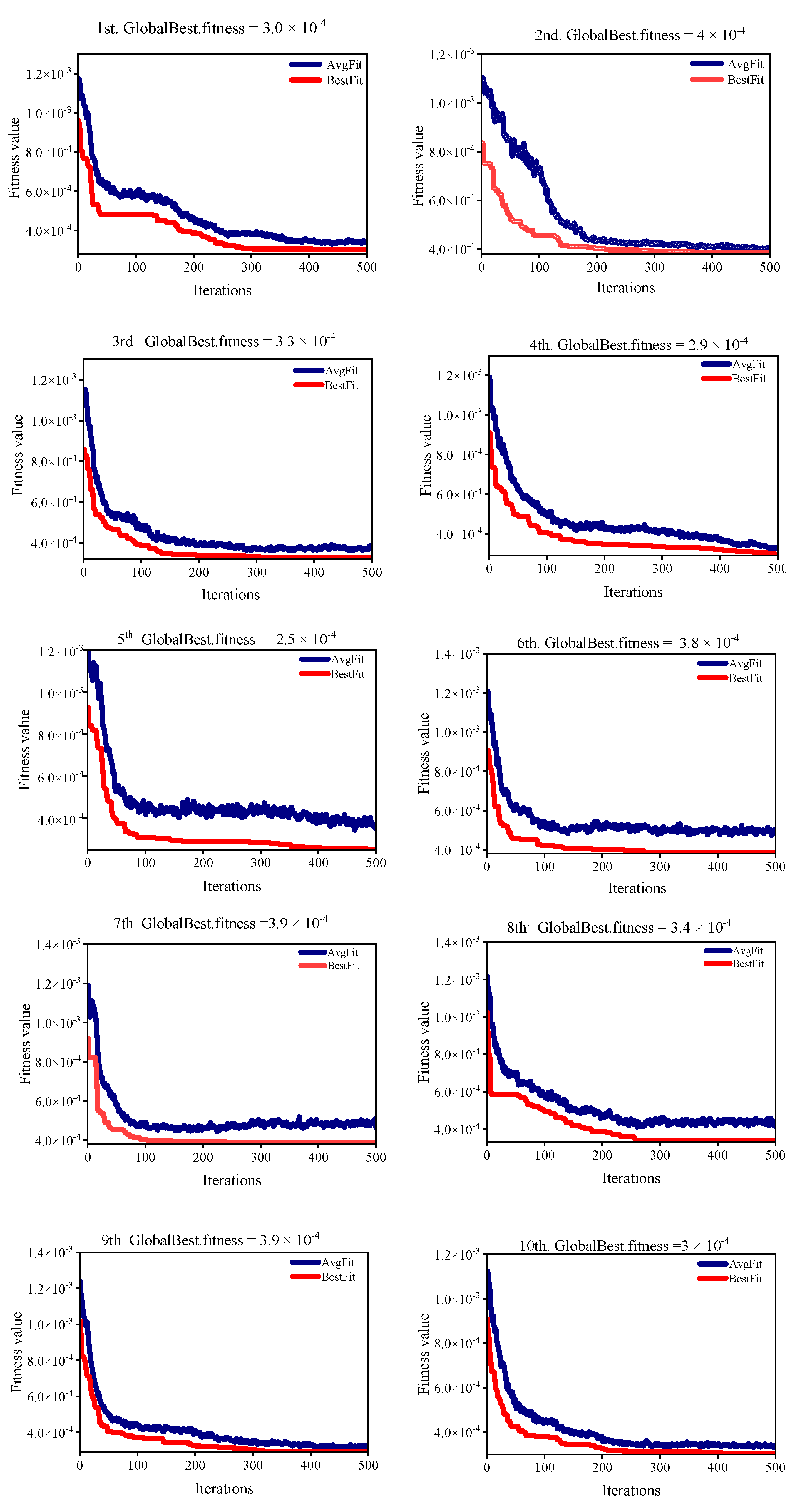
3.1.2. The PSO-BP Neural Network
The Optimized Parameters of the Network Model
Number of Particles in the Population
The Number of Iterations
Inertia Weight
The Inertia Weight Damping Ratio
Acceleration Coefficients
3.2. Model Evaluation Indicators
4. Result and Analysis
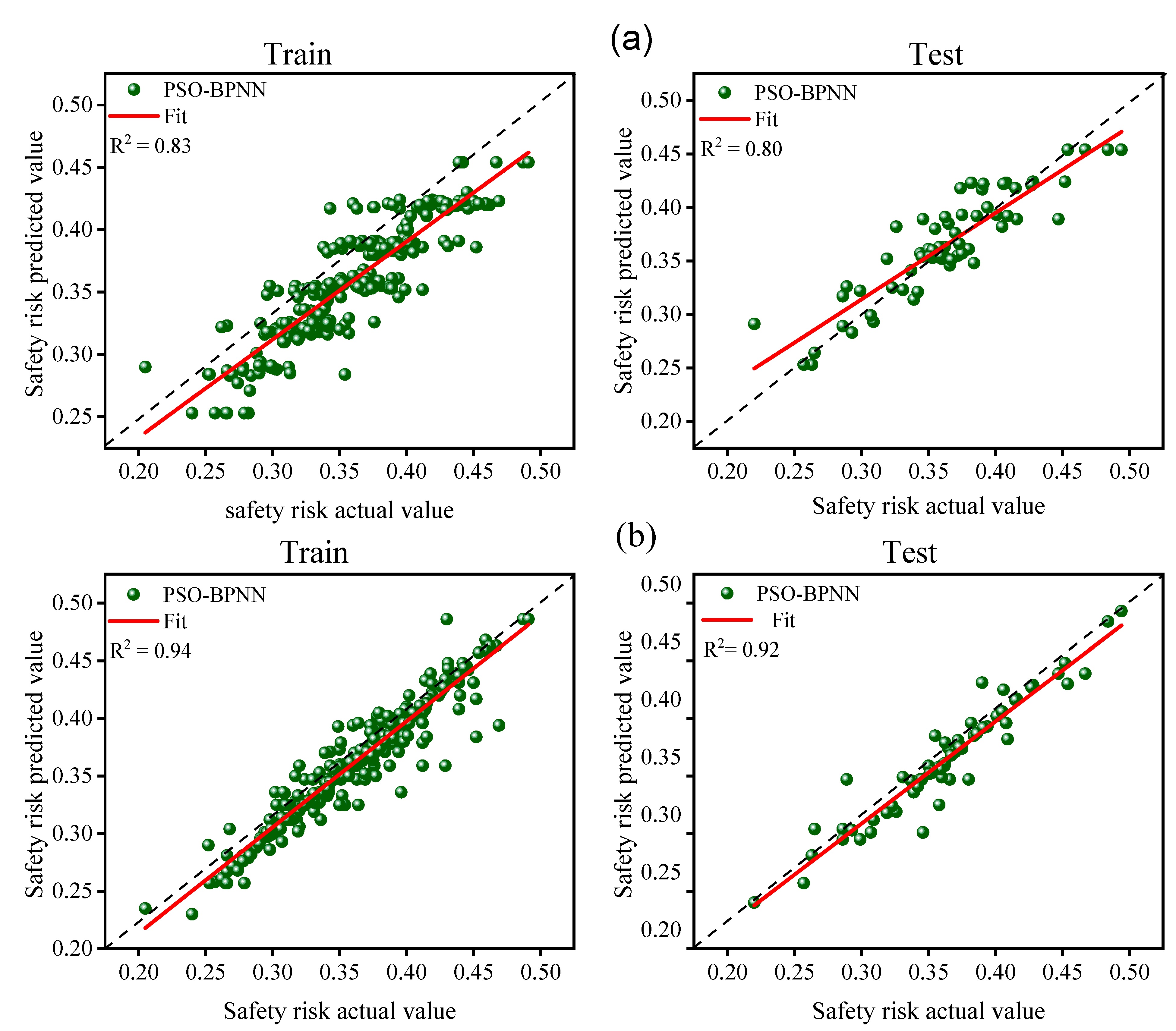
4.1. Results Analysis
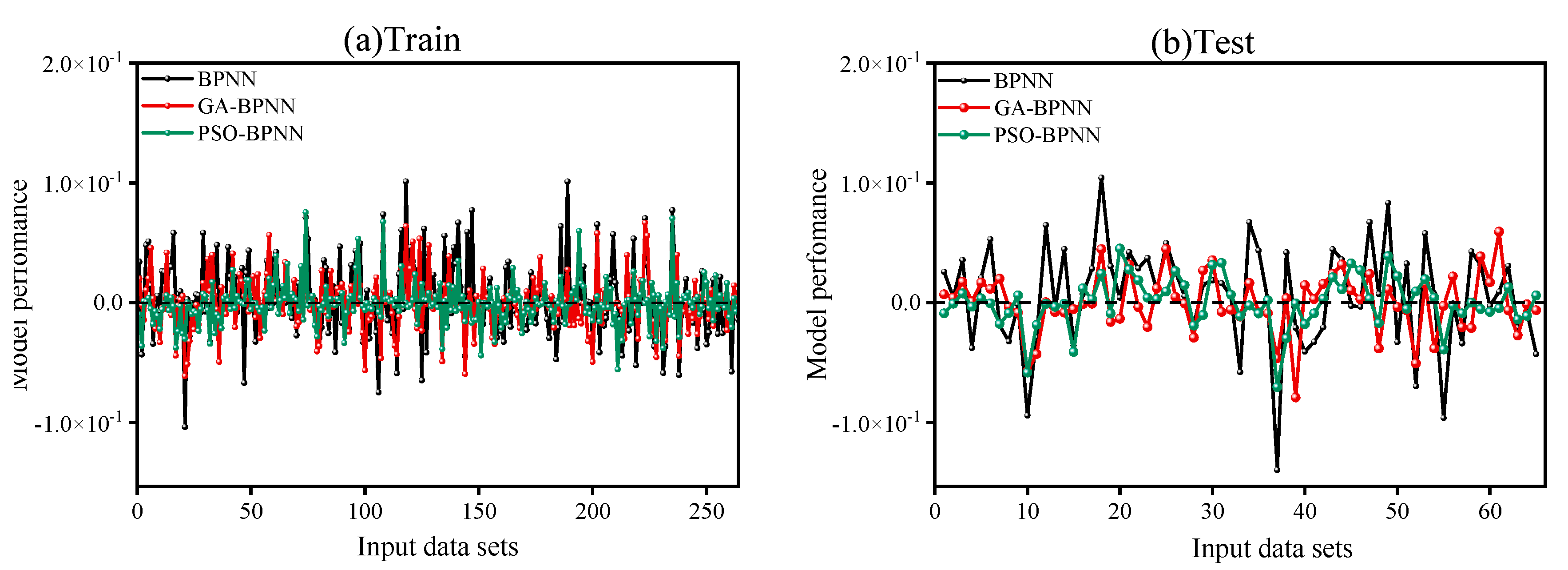
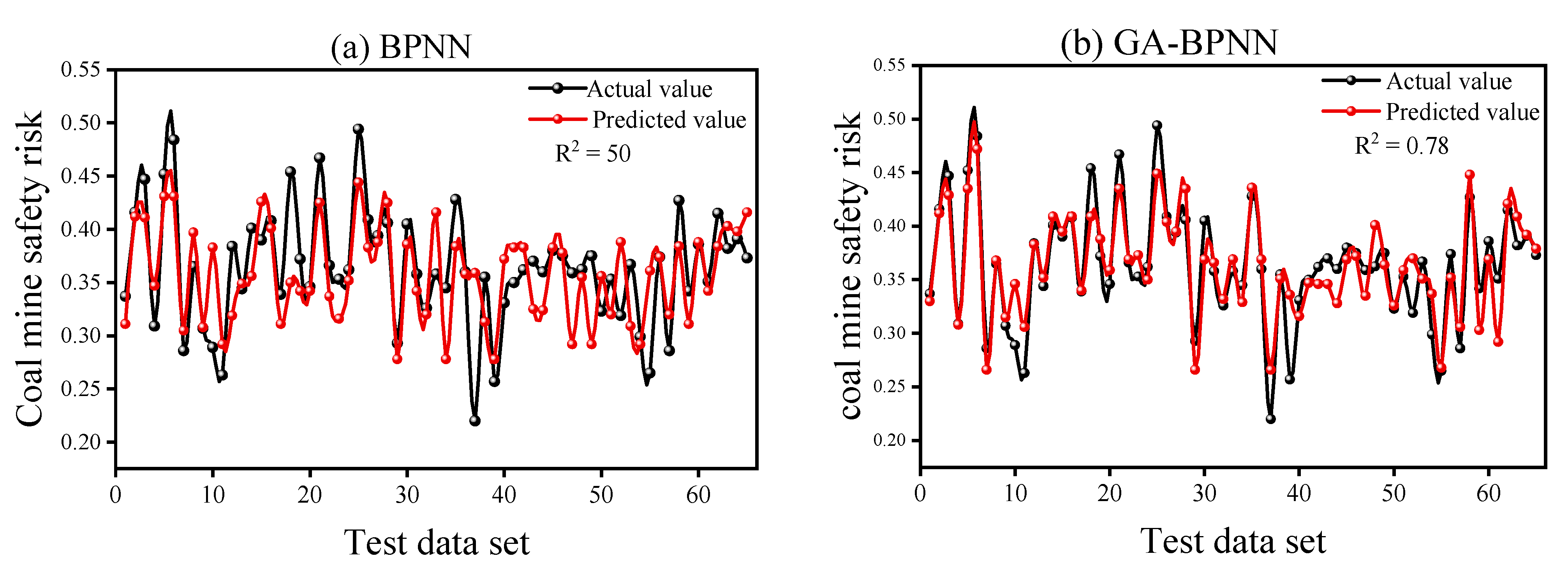
4.2. Comparative Analysis of Models
4.3. Limitations of the Study
5. Conclusions
Author Contributions
Funding
Institutional Review Board Statement
Informed Consent Statement
Data Availability Statement
Acknowledgments
Conflicts of Interest
Abbreviations
| OK | The output vector of the network in the k-ith layer |
| netk | The summation weighted at the output layer k |
| Wjk | The weight of hidden layer j and output layer k |
| yj | The output of the hidden layer j |
| xi | The input at the nodes in layer i |
| νij | The weight of the input layer and hidden layer |
| netj | the summation of the weighted input |
| wjk | The transfer function in the jth layer node |
| The neural network error | |
| The learning constant | |
| The error signal for the output layer O and hidden layer k | |
| Δwjk | Deviation error of the weight in the hidden layer j and output layer k |
| Δνiij | Derivation error of the weight in input layer I and hidden layer j |
| Xi | The position of the ith particle |
| Vi | The velocity of the particle |
| C1 | The personal learning coefficient |
| C2 | The global learning coefficient |
| The inertia weight parameter in the PSO algorithm | |
| Xnorm | Normalized data |
| Coefficient of determination | |
| Mean absolute percentage error | |
| Mean squared error |
References
- Paul, P.S.; Maiti, J. The role of behavioral factors on safety management in underground mines. Saf. Sci. 2007, 45, 449–471. [Google Scholar] [CrossRef]
- Senapati, A.; Bhattacherjee, A.; Chatterjee, S. Causal relationship of some personal and impersonal variates to occupational injuries at continuous miner worksites in underground coal mines. Saf. Sci. 2022, 146, 105562. [Google Scholar] [CrossRef]
- Petsonk, E.L.; Rose, C.; Cohen, R. Coal mine dust lung disease. New lessons from an old exposure. Am. J. Respir. Crit. Care Med. 2013, 187, 1178–1185. [Google Scholar] [CrossRef]
- Sovacool, B.K. The costs of failure: A preliminary assessment of major energy accidents, 1907–2007. Energy Policy 2008, 36, 1802–1820. [Google Scholar] [CrossRef]
- Li, S.; You, M.; Li, D.; Liu, J. Identifying coal mine safety production risk factors by employing text mining and Bayesian network techniques. Process Saf. Environ. Prot. 2022, 162, 1067–1081. [Google Scholar] [CrossRef]
- Wang, D.; Sui, W.; Ranville, J.F. Hazard identification and risk assessment of groundwater inrush from a coal mine: A review. Bull. Eng. Geol. Environ. 2022, 81, 421. [Google Scholar] [CrossRef]
- Tong, R.; Yang, Y.; Ma, X.; Zhang, Y.; Li, S.; Yang, H. Risk assessment of Miners’ unsafe behaviors: A case study of gas explosion accidents in coal mine, china. Int. J. Environ. Res. Public Health 2019, 16, 1765. [Google Scholar] [CrossRef] [PubMed]
- Kharzi, R.; Chaib, R.; Verzea, I.; Akni, A. A Safe and Sustainable Development in a Hygiene and Healthy Company Using Decision Matrix Risk Assessment Technique: A case study. J. Min. Environ. 2020, 11, 363–373. [Google Scholar]
- Hassanien, A.E.; Darwish, A.; Abdelghafar, S. Machine learning in telemetry data mining of space mission: Basics, challenging and future directions. Artif. Intell. Rev. 2020, 53, 3201–3230. [Google Scholar] [CrossRef]
- Ayvaz, S.; Alpay, K. Predictive maintenance system for production lines in manufacturing: A machine learning approach using IoT data in real-time. Expert Syst. Appl. 2021, 173, 114598. [Google Scholar] [CrossRef]
- Kashyap, R. Geospatial Big Data, Analytics and IoT: Challenges, Applications and Potential. In Cloud Computing for Geospatial Big Data Analytics: Intelligent Edge, Fog and Mist Computing; Springer: Berlin/Heidelberg, Germany, 2019; pp. 191–213. [Google Scholar]
- Manzoor, U.; Ehsan, M.; Radwan, A.E.; Hussain, M.; Iftikhar, M.K.; Arshad, F. Seismic driven reservoir classification using advanced machine learning algorithms: A case study from the lower Ranikot/Khadro sandstone gas reservoir, Kirthar fold belt, lower Indus Basin, Pakistan. Geoenergy Sci. Eng. 2023, 222, 211451. [Google Scholar] [CrossRef]
- Sahu, A.; Mishra, D.P. Coal mine explosions in India: Management failure, safety lapses and mitigative measures. Extr. Ind. Soc. 2023, 14, 101233. [Google Scholar] [CrossRef]
- Zheng, Z.; Wang, F.; Gong, G.; Yang, H.; Han, D. Intelligent technologies for construction machinery using data-driven methods. Autom. Constr. 2023, 147, 104711. [Google Scholar] [CrossRef]
- Kudashkina, K.; Corradini, M.G.; Thirunathan, P.; Yada, R.Y.; Fraser, E.D. Artificial Intelligence technology in food safety: A behavioral approach. Trends Food Sci. Technol. 2022, 123, 36–38. [Google Scholar] [CrossRef]
- Sadeghi, S.; Soltanmohammadlou, N.; Nasirzadeh, F. Applications of wireless sensor networks to improve occupational safety and health in underground mines. J. Saf. Res. 2022, 83, 8–25. [Google Scholar] [CrossRef] [PubMed]
- Ali, M.H.; Al-Azzawi, W.K.; Jaber, M.; Abd, S.K.; Alkhayyat, A.; Rasool, Z.I. Improving coal mine safety with internet of things (IoT) based Dynamic Sensor Information Control System. Phys. Chem. Earth Parts A/B/C 2022, 128, 103225. [Google Scholar] [CrossRef]
- Bai, G.; Xu, T. Coal mine safety evaluation based on machine learning: A BP neural network model. Comput. Intell. Neurosci. 2022, 2022, 5233845. [Google Scholar] [CrossRef]
- Cruz, I.A.; Chuenchart, W.; Long, F.; Surendra, K.; Andrade, L.R.S.; Bilal, M.; Liu, H.; Figueiredo, R.T.; Khanal, S.K.; Ferreira, L.F.R. Application of machine learning in anaerobic digestion: Perspectives and challenges. Bioresour. Technol. 2022, 345, 126433. [Google Scholar] [CrossRef]
- Agatonovic-Kustrin, S.; Beresford, R. Basic concepts of artificial neural network (ANN) modeling and its application in pharmaceutical research. J. Pharm. Biomed. Anal. 2000, 22, 717–727. [Google Scholar] [CrossRef]
- Wu, Y.; Gao, R.; Yang, J. Prediction of coal and gas outburst: A method based on the BP neural network optimized by GASA. Process Saf. Environ. Prot. 2020, 133, 64–72. [Google Scholar] [CrossRef]
- Zheng, Y.; Zhong, H.; Fang, Y.; Zhang, W.; Liu, K.; Fang, J. Rockburst prediction model based on entropy weight integrated with grey relational BP neural network. Adv. Civ. Eng. 2019, 2019, 34. [Google Scholar] [CrossRef]
- Qi, S.; Jin, K.; Li, B.; Qian, Y. The exploration of internet finance by using neural network. J. Comput. Appl. Math. 2020, 369, 112630. [Google Scholar] [CrossRef]
- Chong, H.Y.; Yap, H.J.; Tan, S.C.; Yap, K.S.; Wong, S.Y. Advances of metaheuristic algorithms in training neural networks for industrial applications. Soft Comput. 2021, 25, 11209–11233. [Google Scholar] [CrossRef]
- Zhong, K.; Wang, Y.; Pei, J.; Tang, S.; Han, Z. Super efficiency SBM-DEA and neural network for performance evaluation. Inf. Process. Manag. 2021, 58, 102728. [Google Scholar] [CrossRef]
- Yang, L.; Birhane, G.E.; Zhu, J.; Geng, J. Mining employees safety and the application of information technology in coal mining. Front. Public Health 2021, 9, 709987. [Google Scholar] [CrossRef]
- Chen, J.; Huang, S. Evaluation model of green supply chain cooperation credit based on BP neural network. Neural Comput. Appl. 2021, 33, 1007–1015. [Google Scholar] [CrossRef]
- Rumelhart, D.E.; Hinton, G.E.; Williams, R.J. Learning Representations by Backpropagating Errors. Nature 1986, 323, 533–536. [Google Scholar] [CrossRef]
- López-Monroy, A.P.; García-Salinas, J.S. Neural networks and deep learning. In Biosignal Processing and Classification Using Computational Learning and Intelligence; Academic Press: Cambridge, MA, USA, 2022; pp. 177–196. [Google Scholar]
- Jana, D.K.; Bhunia, P.; Adhikary, S.D.; Bej, B. Optimization of effluents using artificial neural network and support vector regression in detergent industrial wastewater treatment. Clean. Chem. Eng. 2022, 3, 100039. [Google Scholar] [CrossRef]
- Shen, S.L.; Elbaz, K.; Shaban, W.M.; Zhou, A. Real-time prediction of shield moving trajectory during tunnelling. Acta Geotech. 2022, 17, 1533–1549. [Google Scholar] [CrossRef]
- Hosseini, V.R.; Mehrizi, A.A.; Gungor, A.; Afrouzi, H.H. Application of a physics-informed neural network to solve the steady-state Bratu equation arising from solid biofuel combustion theory. Fuel 2023, 332, 125908. [Google Scholar] [CrossRef]
- Saeed, A.; Li, C.; Gan, Z.; Xie, Y.; Liu, F. A simple approach for short-term wind speed interval prediction based on independently recurrent neural networks and error probability distribution. Energy 2022, 238, 122012. [Google Scholar] [CrossRef]
- Zhang, S.Z.; Chen, S.; Jiang, H. A back propagation neural network model for accurately predicting the removal efficiency of ammonia nitrogen in wastewater treatment plants using different biological processes. Water Res. 2022, 222, 118908. [Google Scholar] [CrossRef]
- Feng, C.; Zhang, J.; Zhang, W.; Hodge, B.M. Convolutional neural networks for intra-hour solar forecasting based on sky image sequences. Appl. Energy 2022, 310, 118438. [Google Scholar] [CrossRef]
- Rodzin, S.; Bova, V.; Kravchenko, Y.; Rodzina, L. Deep Learning Techniques for Natural Language Processing. In Artificial Intelligence Trends in Systems, Proceedings of the 11th Computer Science On-line Conference, July 2022; Springer International Publishing: Cham, Switzerland, 2022; Volume 2, pp. 121–130. [Google Scholar]
- Wen, T.; Xiao, Y.; Wang, A.; Wang, H. A novel hybrid feature fusion model for detecting phishing scam on Ethereum using deep neural network. Expert Syst. Appl. 2023, 211, 118463. [Google Scholar] [CrossRef]
- Rajawat, A.S.; Jain, S. Fusion deep learning based on back propagation neural network for personalization. In Proceedings of the 2nd International Conference on Data, Engineering and Applications (IDEA), Bhopal, India, 28–29 February 2020; IEEE: New York, NY, USA, 2010; pp. 1–7. [Google Scholar]
- Kennedy, J.; Eberhart, R. Particle swarm optimization. In Proceedings of the IEEE International Conference on Neural Networks, Perth, WA, Australia, 27 November–1 December 1995; Volume 4, pp. 1942–1948. [Google Scholar]
- Pontani, M.; Conway, B.A. Particle swarm optimization applied to space trajectories. J. Guid. Control Dyn. 2010, 33, 1429–1441. [Google Scholar] [CrossRef]
- Jain, M.; Saihjpal, V.; Singh, N.; Singh, S.B. An Overview of Variants and Advancements of PSO Algorithm. Appl. Sci. 2022, 12, 8392. [Google Scholar] [CrossRef]
- Fallahi, S.; Taghadosi, M. Quantum-behaved particle swarm optimization based on solitons. Sci. Rep. 2022, 12, 13977. [Google Scholar] [CrossRef]
- Arrif, T.; Hassani, S.; Guermoui, M.; Sánchez-González, A.; Taylor, R.A.; Belaid, A. GA-GOA hybrid algorithm and comparative study of different metaheuristic population-based algorithms for solar tower heliostat field design. Renew. Energy 2022, 192, 745–758. [Google Scholar] [CrossRef]
- Punyakum, V.; Sethanan, K.; Nitisiri, K.; Pitakaso, R.; Gen, M. Hybrid differential evolution and particle swarm optimization for Multi-visit and Multi-period workforce scheduling and routing problems. Comput. Electron. Agric. 2022, 197, 106929. [Google Scholar] [CrossRef]
- Mousavirad, S.J.; Rahnamayan, S. CenPSO: A novel center-based particle swarm optimization algorithm for large-scale optimization. In Proceedings of the 2020 IEEE International Conference on Systems, Man, and Cybernetics (SMC), Toronto, ON, Canada, 11–14 October 2020; pp. 2066–2071. [Google Scholar]
- Lv, Z.; Wang, L.; Han, Z.; Zhao, J.; Wang, W. Surrogate-assisted particle swarm optimization algorithm with Pareto active learning for expensive multi-objective optimization. IEEE/CAA J. Autom. Sin. 2019, 6, 838–849. [Google Scholar] [CrossRef]
- Premkumar, M.; Jangir, P.; Sowmya, R.; Alhelou, H.H.; Heidari, A.A.; Chen, H. MOSMA: Multi-objective slime mould algorithm based on elitist non-dominated sorting. IEEE Access 2020, 9, 3229–3248. [Google Scholar] [CrossRef]
- Naji, H.R.; Shadravan, S.; Jafarabadi, H.M.; Momeni, H. Accelerating sailfish optimization applied to unconstrained optimization problems on graphical processing unit. Eng. Sci. Technol. Int. J. 2022, 32, 101077. [Google Scholar]
- Robinson, E.; Sutin, A.R.; Daly, M.; Jones, A. A systematic review and meta-analysis of longitudinal cohort studies comparing mental health before versus during the COVID-19 pandemic in 2020. J. Affect. Disord. 2022, 296, 567–576. [Google Scholar] [CrossRef] [PubMed]
- Marini, F.; Walczak, B. Particle swarm optimization (PSO). A tutorial. Chemom. Intell. Lab. Syst. 2015, 149, 153–165. [Google Scholar] [CrossRef]
- Rahnamayan, S.; Wang, G.G. Toward effective initialization for large-scale search spaces. Trans Syst. 2009, 8, 355–367. [Google Scholar]
- Khare, A.; Rangnekar, S. A review of particle swarm optimization and its applications in solar photovoltaic system. Appl. Soft Comput. 2013, 13, 2997–3006. [Google Scholar] [CrossRef]
- Sigarchian, S.G.; Orosz, M.S.; Hemond, H.F.; Malmquist, A. Optimum design of a hybrid PV–CSP–LPG microgrid with Particle Swarm Optimization technique. Appl. Therm. Eng. 2016, 109, 1031–1036. [Google Scholar] [CrossRef]
- Han, W.; Yang, P.; Ren, H.; Sun, J. Comparison study of several kinds of inertia weights for PSO. In Proceedings of the 2010 IEEE International Conference on Progress in Informatics and Computing, Shanghai, China, 1–12 December 2010; IEEE: New York, NY, USA, 2010; Volume 1, pp. 280–284. [Google Scholar]
- Liang, J.J.; Qin, A.K.; Suganthan, P.N.; Baskar, S. Comprehensive learning particle swarm optimizer for global optimization of multimodal functions. IEEE Trans. Evol. Comput. 2006, 10, 281–295. [Google Scholar] [CrossRef]
- Jiao, B.; Lian, Z.; Gu, X. A dynamic inertia weight particle swarm optimization algorithm. Chaos Solitons Fractals 2008, 37, 698–705. [Google Scholar] [CrossRef]
- Eberhart, R.C.; Shi, Y. Comparison between genetic algorithms and particle swarm optimization. In Proceedings of the Evolutionary Programming VII: 7th International Conference, EP98, San Diego, CA, USA, 25–27 March 1998; Springer: Berlin/Heidelberg, Germany, 1998; pp. 611–616. [Google Scholar]
- Parsopoulos, K.E.; Vrahatis, M.N. Recent approaches to global optimization problems through particle swarm optimization. Nat. Comput. 2002, 1, 235–306. [Google Scholar] [CrossRef]
- Clerc, M.; Kennedy, J. The particle swarm-explosion, stability, and convergence in a multidimensional complex space. IEEE Trans. Evol. Comput. 2002, 6, 58–73. [Google Scholar] [CrossRef]
- Deng, G.-F.; Lin, W.-T.; Lo, C.-C. Markowitz-based portfolio selection with cardinality constraints using improved particle swarm optimization. Expert Syst. Appl. 2012, 39, 4558–4566. [Google Scholar] [CrossRef]
- Trivedi, V.; Varshney, P.; Ramteke, M. A simplified multi-objective particle swarm optimization algorithm. Swarm Intell. 2020, 14, 83–116. [Google Scholar] [CrossRef]
- Singh, N.; Singh, S.B.; Houssein, E.H. Hybridizing salp swarm algorithm with particle swarm optimization algorithm for recent optimization functions. Evol. Intell. 2022, 15, 1–34. [Google Scholar] [CrossRef]
- Zhang, M.; Liu, D.; Wang, Q.; Zhao, B.; Bai, O.; Sun, J. Detection of alertness-related EEG signals based on decision fused BP neural network. Biomed. Signal Process. Control 2022, 74, 103479. [Google Scholar] [CrossRef]
- Yu, F.; Xu, X. A short-term load forecasting model of natural gas based on optimized genetic algorithm and improved BP neural network. Appl. Energy 2014, 134, 102–113. [Google Scholar] [CrossRef]
- Ghaffari, A.; Abdollahi, H.; Khoshayand, M.R.; Bozchalooi, I.S.; Dadgar, A.; Rafiee-Tehrani, M. Performance comparison of neural network training algorithms in modeling of bimodal drug delivery. Int. J. Pharm. 2006, 327, 126–138. [Google Scholar] [CrossRef]
- Rodger, J.A. A fuzzy nearest neighbor neural network statistical model for predicting demand for natural gas and energy cost savings in public buildings. Expert Syst. Appl. 2014, 41, 1813–1829. [Google Scholar] [CrossRef]
- Ren, C.; An, N.; Wang, J.; Li, L.; Hu, B.; Shang, D. Optimal parameters selection for BP neural network based on particle swarm optimization: A case study of wind speed forecasting. Knowl. Based Syst. 2014, 56, 226–239. [Google Scholar] [CrossRef]
- Singh, P.; Dwivedi, P. Integration of new evolutionary approach with artificial neural network for solving short term load forecast problem. Appl. Energy 2018, 217, 537–549. [Google Scholar] [CrossRef]
- Lage, P.L.C. An analytical solution to the population balance equation with coalescence and breakage-the special case with constant number of particles. Chem. Eng. Sci. 2002, 53, 599–601. [Google Scholar]
- Shi, X.H.; Liang, Y.C.; Lee, H.P.; Lu, C.; Wang, L.M. An improved GA and a novel PSO-GA-based hybrid algorithm. Inf. Process. Lett. 2005, 93, 255–261. [Google Scholar] [CrossRef]
- Adam, P.P.; Napiorkowski, J.J.; Piotrowska, A.E. Population size in particle swarm optimization. Swarm Evol. Comput. 2020, 58, 100718. [Google Scholar]
- Zhang, H.; Li, H.; Tam, C.M. Particle swarm optimization for resource-constrained project scheduling. Int. J. Proj. Manag. 2006, 24, 83–92. [Google Scholar] [CrossRef]
- Lobo, F.G.; Lima, C.F. Adaptive Population Sizing Schemes in Genetic Algorithms. Parameter Setting Evol. Algorithms 2007, 54, 185–204. [Google Scholar]
- Kentzoglanakis, K.; Poole, M. Particle swarm optimization with an oscillating inertia weight. In Proceedings of the 11th Annual Conference on Genetic and Evolutionary Computation, Montreal, QC, Canada, 8–12 July 2009; pp. 1749–1750. [Google Scholar]
- He, M.; Liu, M.; Wang, R.; Jiang, X.; Liu, B.; Zhou, H. Particle swarm optimization with damping factor and cooperative mechanism. Appl. Soft Comput. 2019, 76, 45–52. [Google Scholar] [CrossRef]
- Rao, R.V.; Pawar, P.J.; Shankar, R. Multi-objective optimization of electrochemical machining process parameters using a particle swarm optimization algorithm. Proc. Inst. Mech. Eng. Part B J. Eng. Manuf. 2008, 222, 949–958. [Google Scholar] [CrossRef]
- Song, Y.; Chen, Z.; Yuan, Z. New chaotic PSO-based neural network predictive control for nonlinear process. IEEE Trans. Neural Netw. 2007, 18, 595–601. [Google Scholar] [CrossRef]
- Gogtay, N.J.; Thatte, U.M. Principles of correlation analysis. J. Assoc. Physicians India 2017, 65, 78–81. [Google Scholar] [PubMed]
- Wang, Z.; Zhang, J.; Wang, J.; He, X.; Fu, L.; Tian, F.; Liu, X.; Zhao, Y. A Back Propagation neural network based optimizing model of space-based large mirror structure. Optik 2019, 179, 780–786. [Google Scholar] [CrossRef]
- Davide, C.; Warrens, M.J.; Jurman, G. The coefficient of determination R-squared is more informative than SMAPE, MAE, MAPE, MSE and RMSE in regression analysis evaluation. PeerJ Comput. Sci. 2021, 7, e623. [Google Scholar]
- Zhu, C.; Zhang, J.; Liu, Y.; Ma, D.; Li, M.; Xiang, B. Comparison of GA-BP and PSO-BP neural network models with initial BP model for rainfall-induced landslides risk assessment in regional scale: A case study in Sichuan, China. Nat. Hazards 2020, 100, 173–204. [Google Scholar] [CrossRef]
- Ma, C.; Zhao, L.; Mei, X.; Shi, H.; Yang, J. Thermal error compensation of high-speed spindle system based on a modified BP neural network. Int. J. Adv. Manuf. Technol. 2017, 89, 3071–3085. [Google Scholar] [CrossRef]
- Deng, Y.; Xiao, H.; Xu, J.; Wang, H. Prediction model of PSO-BP neural network on coliform amount in special food. Saudi J. Biol. Sci. 2019, 26, 1154–1160. [Google Scholar] [CrossRef] [PubMed]
- Lin, S.W.; Chen, S.C.; Wu, W.J.; Chen, C.H. Parameter determination and feature selection for back-propagation network by particle swarm optimization. Knowl. Inf. Syst. 2009, 21, 249–266. [Google Scholar] [CrossRef]
- Jiang, L.; Wang, X. Optimization of online teaching quality evaluation model based on hierarchical PSO-BP neural network. Complexity 2020, 7, 1–12. [Google Scholar] [CrossRef]


| Optimization Parameters | Values |
|---|---|
| The number of particles in the population (SwarmSize) | 50 |
| The maximum number of iterations | 500 |
| Inertia weight (W) | 0.60 |
| The inertia weight damping ratio | 0.40 |
| The personal learning coefficient (C1) | 2.5 |
| The global learning coefficient (C2) | 2.5 |
| Model No. | MSE [×10−4] | MAPE (%) | R2 | |||
|---|---|---|---|---|---|---|
| Train | Test | Train | Test | Train | Test | |
| 1 | 2.9 | 3.7 | 4.1 | 4.7 | 0.84 | 0.83 |
| 2 | 5.4 | 5.5 | 5.0 | 5.1 | 0.83 | 0.80 |
| 3 | 3.5 | 2.6 | 3.6 | 4.9 | 0.86 | 0.84 |
| 4 | 3.5 | 3.0 | 4.3 | 4.2 | 0.85 | 0.86 |
| 5 | 1.1 | 2.0 | 1.2 | 2.6 | 0.94 | 0.92 |
| 6 | 3.7 | 3.8 | 3.6 | 4.8 | 0.87 | 0.91 |
| 7 | 3.5 | 4.3 | 4.3 | 4.2 | 0.88 | 0.87 |
| 8 | 2.1 | 2.3 | 4.0 | 3.7 | 0.85 | 0.81 |
| 9 | 2.4 | 3.9 | 3.7 | 4.1 | 0.87 | 0.83 |
| 10 | 2.2 | 2.3 | 3.7 | 4.7 | 0.83 | 0.85 |
| Model | MSE | MAPE (%) | R2 | |||
|---|---|---|---|---|---|---|
| Train | Test | Train | Test | Train | Test | |
| BPNN | 1.3 × 10⁻³ | 1.5 × 10⁻³ | 6 | 9.7 | 0.64 | 0.50 |
| GA-BPNN | 3.2 × 10⁻⁴ | 4.2 × 10⁻⁴ | 4.2 | 5.1 | 0.82 | 0.78 |
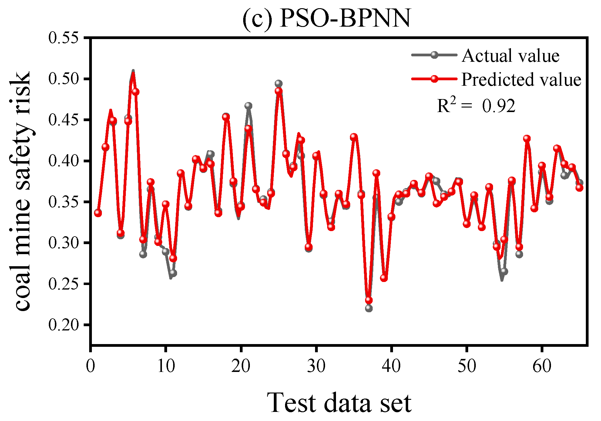
| PSO-BPNN | 1.1 × 10⁻⁴ | 2.0 × 10⁻⁴ | 3.1 | 4.3 | 0.94 | 0.92 |
| Model Prediction Improvement | ||
|---|---|---|
| Train | Test | |
| GA-BPNN | 58.9% | 65.7% |
| PSO-BPNN | 89.3% | 85.2% |
Disclaimer/Publisher’s Note: The statements, opinions and data contained in all publications are solely those of the individual author(s) and contributor(s) and not of MDPI and/or the editor(s). MDPI and/or the editor(s) disclaim responsibility for any injury to people or property resulting from any ideas, methods, instructions or products referred to in the content. |
© 2023 by the authors. Licensee MDPI, Basel, Switzerland. This article is an open access article distributed under the terms and conditions of the Creative Commons Attribution (CC BY) license (https://creativecommons.org/licenses/by/4.0/).
Share and Cite
Mulumba, D.M.; Liu, J.; Hao, J.; Zheng, Y.; Liu, H. Application of an Optimized PSO-BP Neural Network to the Assessment and Prediction of Underground Coal Mine Safety Risk Factors. Appl. Sci. 2023, 13, 5317. https://doi.org/10.3390/app13095317
Mulumba DM, Liu J, Hao J, Zheng Y, Liu H. Application of an Optimized PSO-BP Neural Network to the Assessment and Prediction of Underground Coal Mine Safety Risk Factors. Applied Sciences. 2023; 13(9):5317. https://doi.org/10.3390/app13095317
Chicago/Turabian StyleMulumba, Dorcas Muadi, Jiankang Liu, Jian Hao, Yining Zheng, and Heqing Liu. 2023. "Application of an Optimized PSO-BP Neural Network to the Assessment and Prediction of Underground Coal Mine Safety Risk Factors" Applied Sciences 13, no. 9: 5317. https://doi.org/10.3390/app13095317
APA StyleMulumba, D. M., Liu, J., Hao, J., Zheng, Y., & Liu, H. (2023). Application of an Optimized PSO-BP Neural Network to the Assessment and Prediction of Underground Coal Mine Safety Risk Factors. Applied Sciences, 13(9), 5317. https://doi.org/10.3390/app13095317