Automatic Interpretation of Potential Field Data Based on Euler Deconvolution with Linear Background

Featured Application

Our method can be applied to gravity and magnetic data to obtain the distribution of underground field sources and fault structural characteristics. Additionally, compared with traditional Euler deconvolution, it can obtain more reliable Euler solutions.

Abstract

Euler deconvolution is a popular technique used for analyzing potential field data because it requires little prior information. However, the reliability of Euler solutions can be impacted by interference from adjacent field sources, or background fields. In this manuscript, we present an effective Euler deconvolution algorithm that accounts for linear background fields. Our algorithm, called improved finite-difference Euler deconvolution, builds upon the finite-difference method and is less susceptible to interference from nearby sources. We use this algorithm to achieve a joint estimation of the coefficients of the source coordinates, the structure index, and the linear background trend. Compared to Euler deconvolution methods based on differential similarity transformations, which also account for linear background fields, our method is easier to understand and implement programmatically and is faster. We tested our method using both 2D and 3D synthetic data, and the results indicate that our algorithm has better computational accuracy than the finite-difference algorithm and is comparable to the Euler deconvolution algorithm based on differential similarity transformations. In addition, our method was shown to be effective when tested on real data.

1. Introduction

Gravity exploration and magnetic exploration are the earliest and most widely used methods of geophysical exploration. They have been applied in mineral exploration, oil and gas surveys, and the geological mapping of different scales. In the above-mentioned applications, the calculation of the depth of the field source is one of the most important interpretation objectives, for which a number of automated methods have been proposed to quickly determine the depth, width, horizontal position and shape index of a geological body. The most widely used among these methods are Werner deconvolution [1,2,3], Euler deconvolution [4,5,6,7], analytic signal [8,9,10,11] and DEXP [12,13]. Among these methods, Euler deconvolution does not require a priori knowledge about anomalous source magnetization as far as it is homogeneous throughout the anomalous body and requires neither high-speed computers nor efficient algorithms.

Euler deconvolution is a semiautomatic interpretation technique proposed by Reid et al. [5] which allows the fast processing of large data sets. The technique is based on the Euler equation for homogeneous functions and relates potential field measurements and their gradients. In Euler deconvolution, a sliding data window operator is applied in a piecewise way over the whole data set. Using the measured data inside the window, Euler deconvolution estimates the source positions by solving linear equations. However, because of the interference from adjacent field sources (background field data), the calculated solution is inconsistent with the source position. The background field is one of the main factors affecting the accuracy of inversion results. To reduce its influence, many methods have been developed. These methods can generally be divided into three categories.

Firstly, taking into account a constant background, the method that was developed earliest is the most popularly applied way to deal with background. Thompson [4] creatively added a constant term to the Euler equation to correct the deviation of the inversion result, and this indeed reduces the influence of background on Euler solutions to a certain degree. Reid et al. [5] implemented Thompson’s suggested approach to gridded data. After that, many people adopted this strategy, which treats the background field as a constant. Hsu [14] used the high-order vertical derivative of the anomaly to replace the measured anomaly for Euler deconvolution. The Hilbert transform of constant is zero, and Nabighian and Hansen [15] used the Hilbert transform of the anomaly to replace the measured anomaly in Euler deconvolution. Gerovska [16] considered the product of the structural index (SI) and background as a constant and proposed a finite-difference Euler deconvolution algorithm based on the finite-difference method. To some extent, the accuracy of inversion results was improved by taking the background field as constant. However, the background field data actually varies with the coordinates.

Second, taking into account a linear background, Stavrev [17] proposed a Euler algorithm based on the properties of the differential similarity transformation (DST), and the algorithm linearizes Euler’s equation in the case of a linear background. When the central point of similarity (CPS) coincides with the source singular point, the operator becomes a zero at all observation points. Gerovska et al. proposed two algorithms: MaGSoundDST [18] and MaGSoundFDST [19]. MaGSoundDST is also based on the differential similarity transformation, and when the CPS coincides with a source’s singular point, the property of DST of a magnetic or a gravity anomaly becomes zero or linear at observation points. In each sliding window, a series of assumed structural indices are used to calculate a 3D function that evaluates the linearity of the DST. MaGSoundFDST is based on the linearity of the finite-difference similarity transformation. When the central point of similarity (CPS) of the transformation coincides with a source field’s singular point and a correct N value is used, the FDST of a potential field anomaly becomes zero or linear at all observation points. In each sliding window, a field measured at two different observation levels and a set of structural indices are needed. The three methods described above are among the few algorithms that account for a linear background. In terms of anti-interference ability against noise, MaGSoundFDST is better than the MaGSoundDST and DST algorithms, because it does not need derivatives of measured data. In terms of calculation speed, DST is faster [19,20]. In general, the calculation accuracy of the Euler solutions that take into account linear background is better than that of the first-class algorithms.

Third, taking into account a nonlinear background, Pasteka [21] introduced an interference polynomial to the right-hand side of the Euler equation to reduce the influence of the background field. Dewangan [22] proposed a Euler deconvolution with a nonlinear background. The background is approximated using a rational function, and a nonlinear optimization technique (e.g., precondition conjugate gradient) is applied to calculate the solutions. Up to now, few authors apply the Euler deconvolution with nonlinear background to real data.

In this paper, we propose a new method to improve the accuracy of Euler inversion results, which is less susceptible to interference from nearby sources. The proposed method is based on the finite-difference algorithm and can estimate depth, shape, and the coefficient of the background field simultaneously. In addition, we applied the new approach to 2D and 3D datasets.

2. Methodology

The classical formulation of Euler deconvolution can be written as

$$x_0\frac{\partial T}{\partial x}+y_0\frac{\partial T}{\partial y}+z_0\frac{\partial T}{\partial z}-N(T-B)=x\frac{\partial T}{\partial x}+y\frac{\partial T}{\partial y}+z\frac{\partial T}{\partial z}$$

(1)

where x, y and z are the observation positions. $T,\frac{\partial T}{\partial x},\frac{\partial T}{\partial y}\mathrm{and}\frac{\partial T}{\partial z}$ are the potential field data and their gradients with respect to the variables x, y, and z. x₀, y₀ and z₀ are the source positions. B is the background value, and N is the structural index (SI).

In Euler deconvolution, the SI is generally assumed to be constant in each sliding-window. Assuming that for all the points in a window the background B is constant, the product of N and B are constant and we can write

$$NB=(x_c-x_0)(\frac{\partial T}{\partial x}{)}_c+(y_c-y_0\left)\right(\frac{\partial T}{\partial y}{)}_c+(z_c-z_0)(\frac{\partial T}{\partial z}{)}_c+N{T}_c$$

(2)

where c is the central window point. Substituting Equation (2) into Equation (1), we can obtain

$$\begin{array}{c}{x}_0(\frac{\partial T_i}{\partial x}-\frac{\partial T_c}{\partial x})+y_0(\frac{\partial T_i}{\partial y}-\frac{\partial T_c}{\partial y})+z_0(\frac{\partial T_i}{\partial z}-\frac{\partial T_c}{\partial z})-N(T_i-T_c)\\ =x_i\frac{\partial T_i}{\partial x}+y_i\frac{\partial T_i}{\partial y}+z_i\frac{\partial T_i}{\partial z}-x_c\frac{\partial T_c}{\partial x}-y_c\frac{\partial T_c}{\partial y}-z_c\frac{\partial T_c}{\partial z}\end{array}$$

(3)

where i is the window point. Equation (3) is linear with an unknown source position and SI, and the least squares method can be applied to solve the unknown parameters. It is the basic equation of the finite-difference Euler deconvolution algorithm proposed by Gerovska [16]. However, the method limits itself to accounting for only a constant background.

To some extent, the finite-difference Euler deconvolution method improves the accuracy of Euler solutions. However, the background field is not constant and always varies with the position. In Euler deconvolution, 5~10 times the grid interval may be a good choice for the window size [23] and we consider approximating the background as a linear function in a window more realistic, especially in the case of closely located anomalies that interfere with each other. In this paper, we assume that $B=ax+by+cz+d$, and that NB varies with x, y, and z. Substituting B into Equation (1),

$$\begin{array}{c}{x}_0(\frac{\partial T}{\partial x}-a)+y_0(\frac{\partial T}{\partial y}-b)+z_0(\frac{\partial T}{\partial z}-c)-N(T-ax-by-cz-d)\\ =x(\frac{\partial T}{\partial x}-a)+y(\frac{\partial T}{\partial y}-b)+z(\frac{\partial T}{\partial z}-c)\end{array}$$

(4)

In Equation (4), d is constant and hence, N*d can be treated as a constant. Based on the finite-difference Euler deconvolution algorithm, for all the window locations, we can write

$$\begin{array}{l}Nd=x_c\frac{\partial T_c}{\partial x}+y_c\frac{\partial T_c}{\partial y}+z_c\frac{\partial T_c}{\partial z}-x_0\frac{\partial T_c}{\partial x}-y_0\frac{\partial T_c}{\partial y}-z_0\frac{\partial T_c}{\partial z}+a{x}_0+b{y}_0+c{z}_0\\ +N{T}_c-Na{x}_c-Nb{y}_c-Nc{z}_c-a{x}_c-b{y}_c-c{z}_c\end{array}$$

(5)

c is the central window point. Substituting Nd into Equation (4), we can obtain a new formula:

$$\begin{array}{l}{x}_0(\frac{\partial T_i}{\partial x}-\frac{\partial T_c}{\partial x})+y_0(\frac{\partial T_i}{\partial y}-\frac{\partial T_c}{\partial y})+z_0(\frac{\partial T_i}{\partial z}-\frac{\partial T_c}{\partial x})+a(N+1\left)\right(x_i-x_c)\\ +b(N+1\left)\right(y_i-y_c)+c(N+1\left)\right(z_i-z_c)+N(T_c-T_i)\\ =x_i\frac{\partial T_i}{\partial x}+y_i\frac{\partial T_i}{\partial y}+z_c\frac{\partial T_i}{\partial z}-x_c\frac{\partial T_c}{\partial x}-y_c\frac{\partial T_c}{\partial y}-z_c\frac{\partial T_c}{\partial z}\end{array}$$

(6)

The obtained equation, Equation (6), derived from Euler’s homogeneity equation for a case when the measured field contains a homogeneous anomalous field and a linear background, B is linear to the coordinates of the field source. Therefore, the source parameters and the coefficient of the background field can be estimated simultaneously. If N is given, there are only six unknown parameters, which can be obtained by solving overdetermined equations.

If we make the following abbreviations,

$$\begin{array}{l}\delta T_{xi}=\frac{\partial T_i}{\partial x}-\frac{\partial T_c}{\partial x},\delta T_{yi}=\frac{\partial T_i}{\partial y}-\frac{\partial T_c}{\partial y},\delta T_{zi}=\frac{\partial T_i}{\partial z}-\frac{\partial T_c}{\partial z}\\ \delta T_i=T_i-T_c,\delta x=x_i-x_c,\delta y=y_i-y_c,\delta z=z_i-z_c,\\ \delta xyT{=}_i\frac{\partial T_i}{\partial x}+y_i\frac{\partial T_i}{\partial y}+z_c\frac{\partial T_i}{\partial z}-x_c\frac{\partial T_c}{\partial x}-y_c\frac{\partial T_c}{\partial y}-z_c\frac{\partial T_c}{\partial z}\end{array}$$

(7)

from Equation (6) for every grid point of a sliding window, we obtain

$$\begin{array}{l}{x}_0\delta T_{xi}+y_0\delta T_{yi}+z_0\delta T_{zi}+a(N+1)\delta x+\\ b(N+1)\delta y+c(N+1)\delta z+N\delta T_i=\delta xyT\end{array}$$

(8)

or, in a matrix form,

$$\mathrm{Gp}=\mathrm{y}$$

(9)

where p represents the unknown parameters, G is a coefficient matrix, composed of the field anomaly, the gradient of the anomaly and the coordinate points within the window, and y is a vector of the sums of the product differences of the coordinates and the respective gradients of the field. The least squares value of p is given by

$$\mathrm{p}=({\mathrm{G}}^{\mathrm{T}}\mathrm{G}{)}^{-1}{\mathrm{G}}^{\mathrm{T}}\mathrm{y}$$

(10)

Theoretically, the background function can be regarded as a higher-order functional form (e.g., 2-order or 3-order) and the finite-difference method can still be applied to the Euler equation. Owing to the complexity and unknown nature of the background function, the variation form of the function is unknown. When the selected window size is large, treating the background function as a high-order case is reasonable. However, a large window size may lead to missing small-scale field sources. Therefore, in practical applications, the window size should not be too large. Windows containing between 5 × 5 and 10 × 10 grid points may be the best choice [23]. If the selected order of the background field is high (e.g., 2, 3, etc.), it will lead to overfitting and more valuable anomalies being separated, and this will eventually lead to inaccurate inversion results. Hence, accounting for a linear background in the anomalous field, the Euler deconvolution may perform well in the presence of interfering fields.

In the next section, we will compare the inversion accuracy of our algorithm with that of the Euler inversion algorithm based on DST and the finite-difference Euler deconvolution algorithm.

3. Model Test

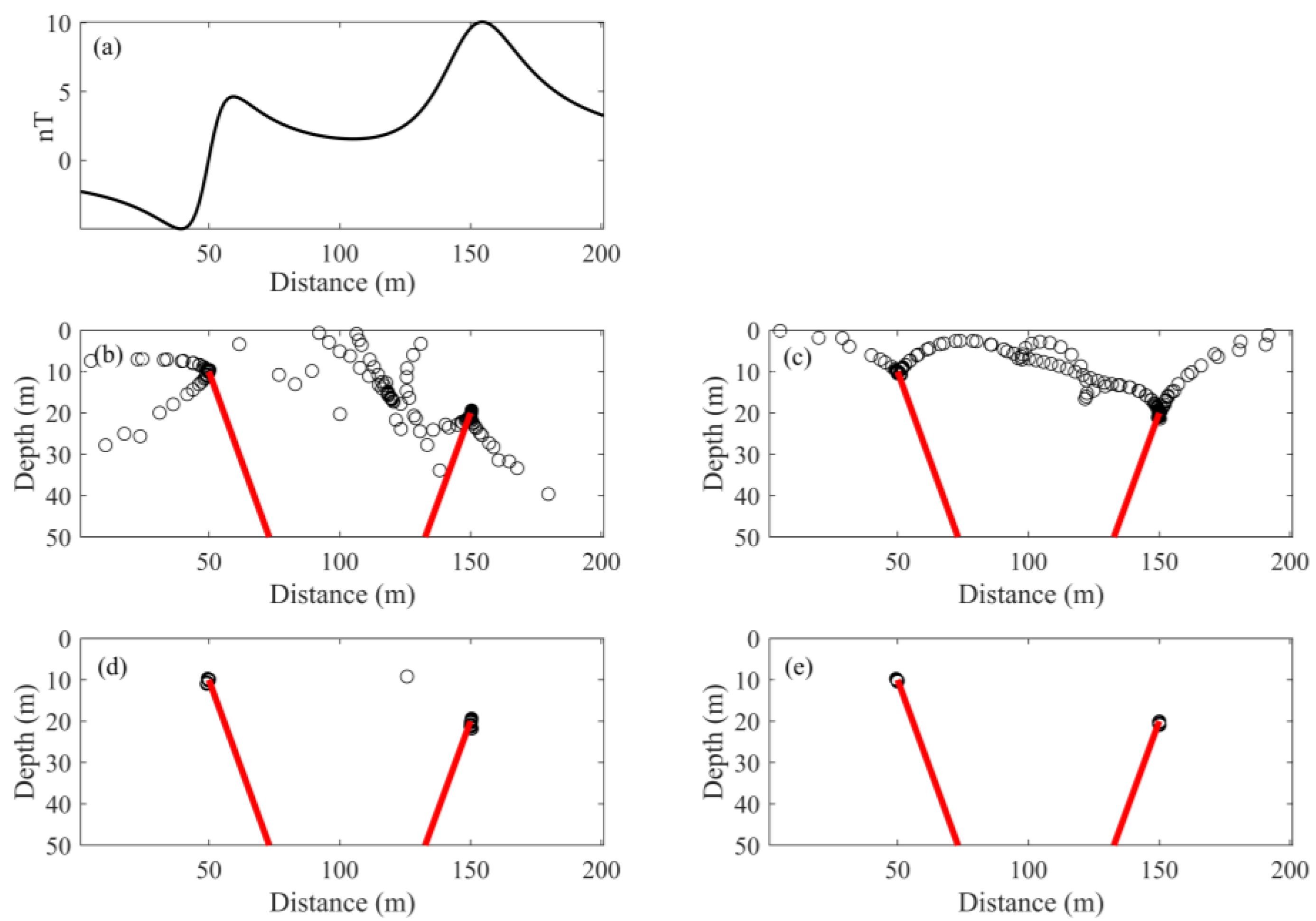
3.1. Test 1: Two Dykes Model Test

To test our method, 2D model data were used, and they were generated from the original code that Cooper [24] provided. Figure 1a shows the synthetic magnetic profile generated by two dykes (I = −60°; D = −22°). Figure 1b,c shows the original inversion results generated by the finite-difference Euler deconvolution algorithm and the improved algorithm, respectively. After performing the two Euler deconvolution algorithms, the moving-rate selection method (Liu et al. [25,26]) with the same parameter was applied to select solutions. The basic idea of the selection method is that when the sliding windows are near the source, the solutons are almost the same. If the distance between the Euler results produced by adjacent windows is less than n times the grid spacing (n < 1), the solutions will be saved. Figure 1d,e shows the results after distinguishing them from Figure 1b,c. According to Figure 1b–e, we can easily find that our method has higher accuracy. For noise-corrupted data (0.5% random Gaussian noise), our method can still produce more reliable solutions (Figure 2).

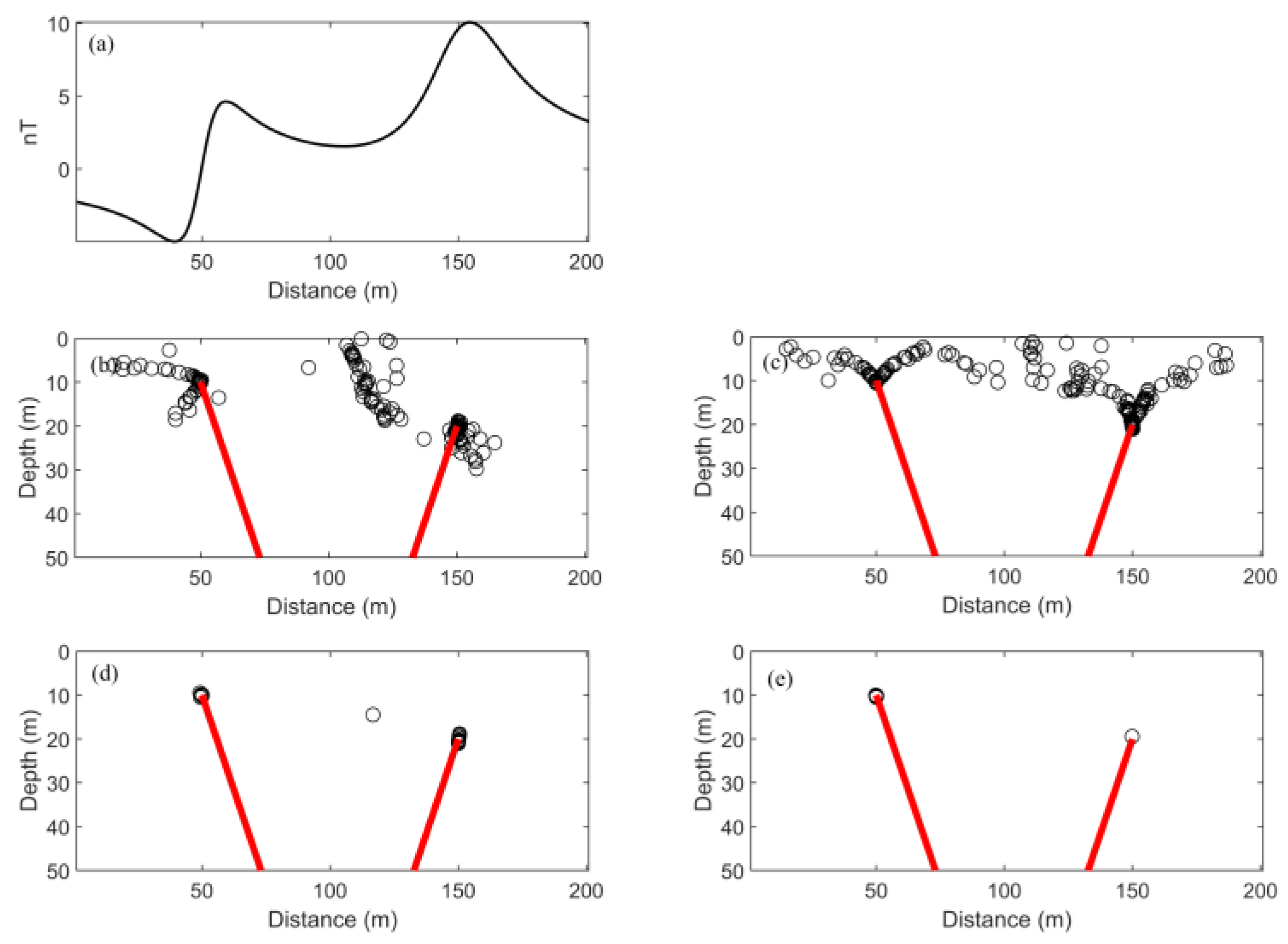
3.2. Test 2: Linear Background

Here, we use a synthetic example with a linear background field with a trend to test our algorithm. Gravity anomaly is produced by a vertical prism, and a linear background is added to the original data (Figure 3). The geometric and physical parameters of this model are listed in

Table 1. Parameters of model 2.

Length along x (km)	Length along y (km)	Thickness along z (km)	Depth to Top (m)	Density (g/cm3)
20	20	5	1.5	0.3

. The grid interval is 1.2 km.

When performing Euler deconvolution, a window size of 11 × 11 is selected and solutions are rejected if the vertical derivative of gravity at the center of the window is negative. Figure 4a displays the original results obtained by applying finite-difference Euler deconvolution to the data in Figure 3c. Figure 4b exhibits the original results obtained by applying the improved finite-difference Euler deconvolution method to the data in Figure 3c. Figure 4c shows the original results obtained by applying Euler deconvolution based on DST to the data in Figure 3c. The selected solutions in Figure 4a–c are shown in Figure 4d,e. The results indicate that our method can better distinguish abnormal boundaries compared to finite-difference Euler deconvolution. Moreover, the distribution of solutions generated by our method and DST Euler deconvolution is almost identical.

Noisy Data

Figure 3d shows the theoretical anomaly corrupted with (1%) random Gaussian noise. In this section, solutions are only saved if the vertical derivative of gravity of the window center is positive. The original Euler solutions, produced by finite-difference Euler deconvolution, our method, and DST Euler deconvolution, are presented in Figure 5a–c. The results, after being selected according to the above criterion, are shown in Figure 5d–f. Based on the data from Figure 5, it can be observed that the distribution of Euler solutions generated by our method and that generated by the DST method are nearly identical.

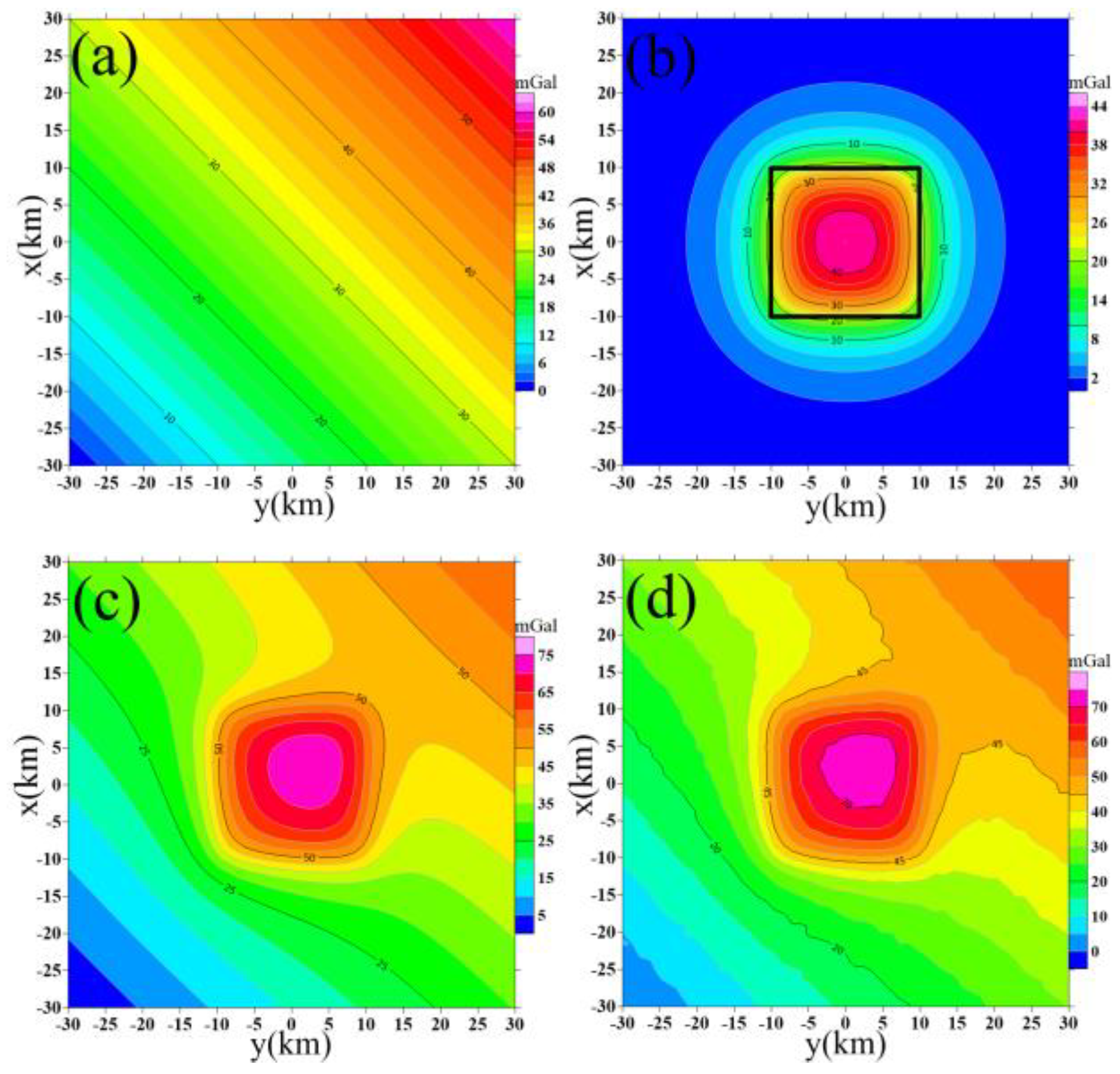
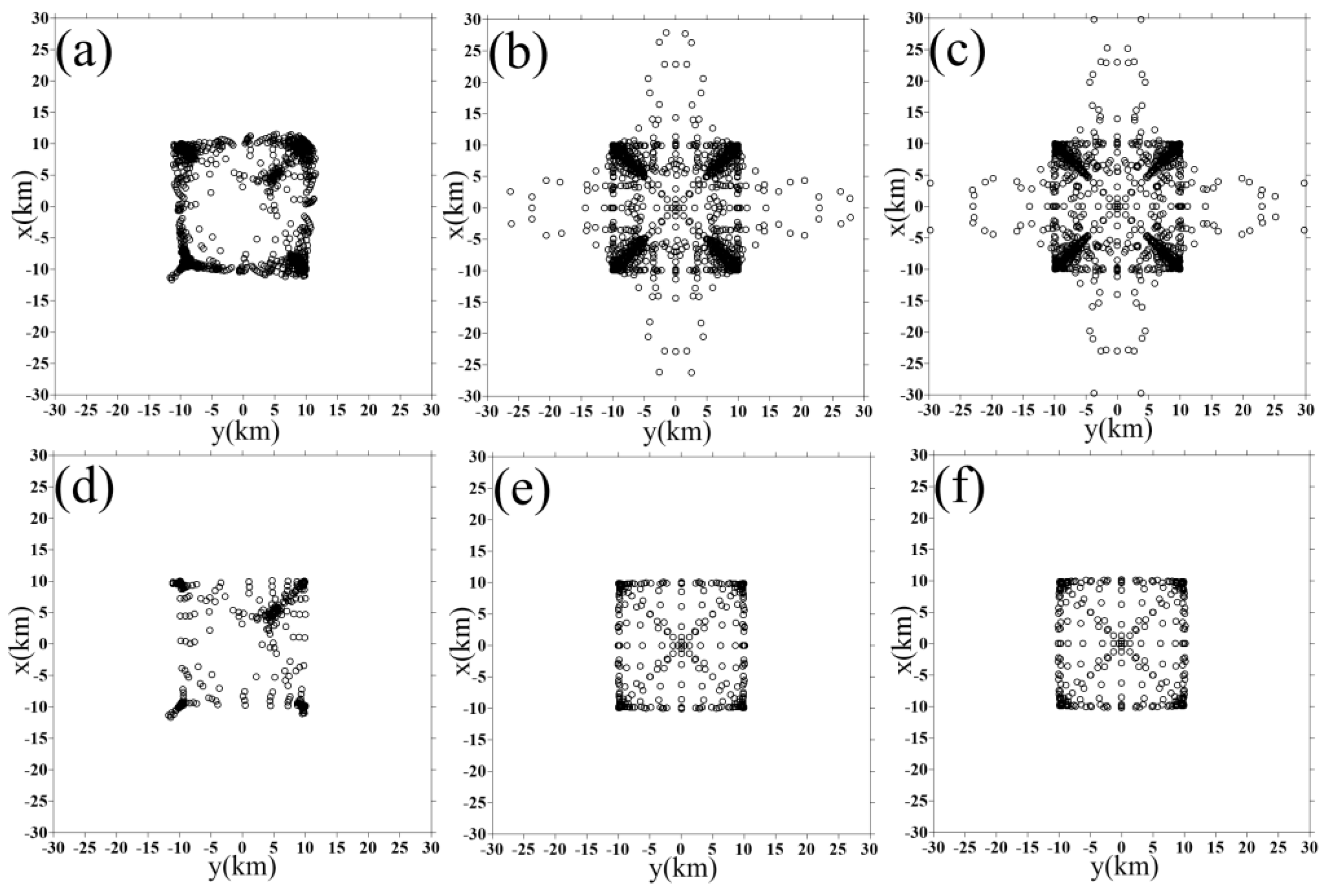
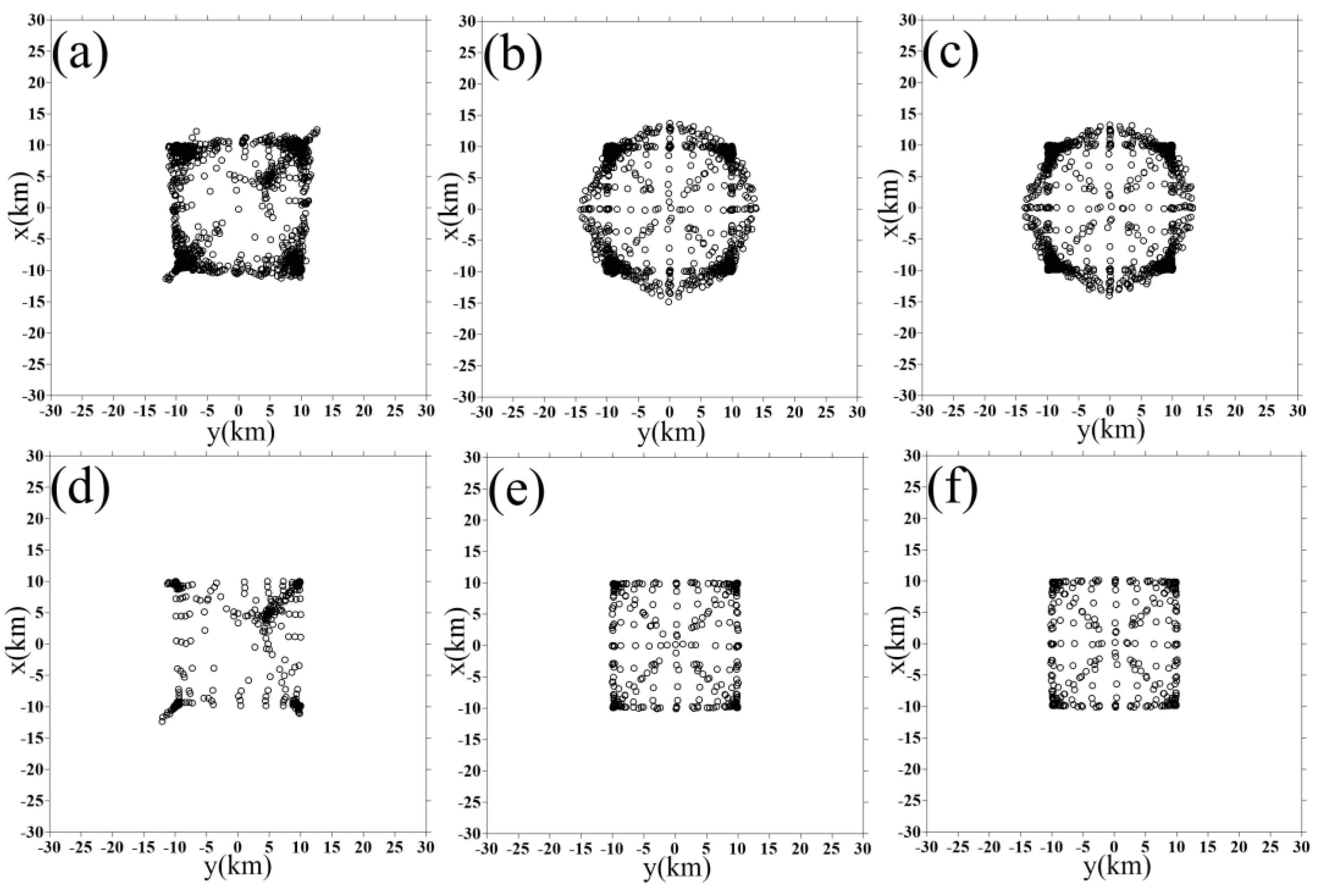
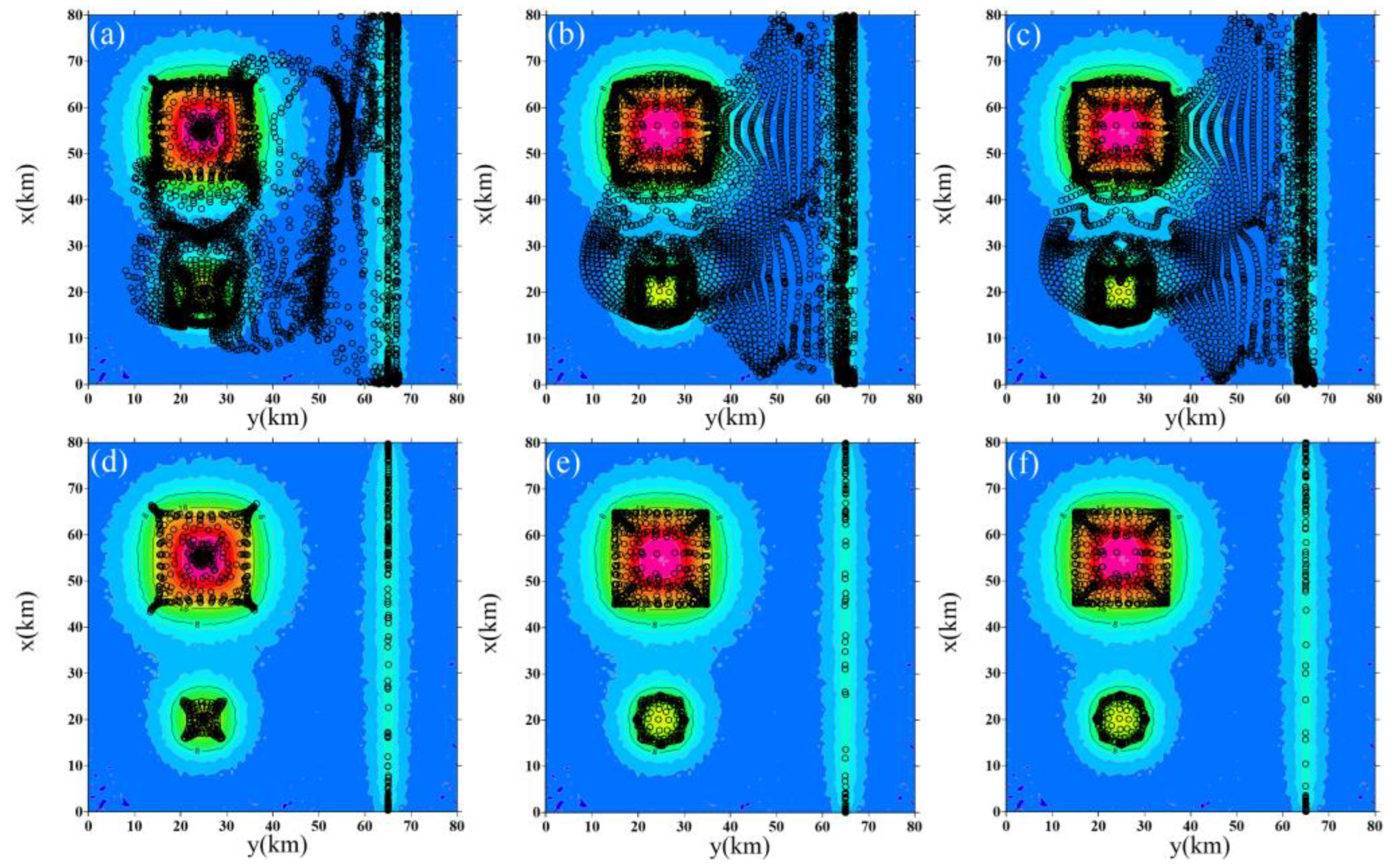
3.3. Test 3: Vertical Prisms Model Test

The third model test contains three vertical prisms. This is the same model used to test new ways to improve the confidence of structural interpretation by an improved Euler inversion and phase congruency method for the field data by Wang et al. [27]. The geometric and physical parameters of this model are listed in

Table 2. Parameters of model 3.

Cuboid No.	Length along x (km)	Length along y (km)	Thickness along z (km)	Depth to Top (m)	Density (g/cm3)
A1	20	20	5	1.5	0.3
A2	10	10	4	2	0.3
A2	80	1	5	1	0.3

. Figure 6a shows the gravity anomaly resulting from these prisms. The input data grid has 101 × 101 points.

Solutions are calculated using a window size of 7 × 7 grid points and solutions are rejected if the vertical derivative of gravity of the window center is negative. Figure 7a shows the original results obtained from applying the finite-difference Euler deconvolution to the data in Figure 6. Figure 7d shows the results after selection. Figure 7b shows the original results obtained from applying the improved Finite-difference Euler deconvolution method to the data in Figure 6. Figure 7e shows the results after selection. Figure 7c shows the original results obtained from applying the Euler deconvolution based on DST to the data in Figure 6a. Figure 7f shows the results after selection.

Comparing Figure 7d and Figure 7e (or Figure 7a and Figure 7b), we can easily find that our algorithm better depicts the boundary of the prisms, and the inversion result is more accurate. Next, we will compare the inversion effects of the improved finite-difference Euler deconvolution method and Euler deconvolution based on DST. Comparing Figure 7e and Figure 7f (or Figure 7b and Figure 7c), we can find that the distribution shapes of the solutions generated by the two algorithms are almost the same. In Figure 7e,f, the mean value of all the x_0-estimate is 39,617 and 39,397, and the mean value of all the y_0-estimate is 39,161 and 38,898. The difference is less than the grid spacing. For these two methods, the difference of z_0-estimate is also far less than the grid interval. The difference in the mean value of the estimated x₀, y₀, and z₀ in Figure 7b,c is also far smaller than the grid interval. To further compare the accuracy of the two algorithms, two profiles are selected. Figure 8 shows the solutions. When the sliding window is in or near the projection area of field sources A1 and A2, the solutions generated from our algorithm and the DST Euler deconvolution algorithm are the same. However, when the sliding window is in or near the projection area of source A3, the solutions generated from the two algorithms are slightly different, and they also reflect the source position.

Noisy Data

To further test the stability of our method, we apply it to noise-corrupted data. Figure 6b shows the gravity anomaly corrupted with (2%) random Gaussian noise. Figure 9 shows the results of the Euler deconvolution methods. Based on the results, we find that, in contrast with solutions generated by the finite-difference Euler deconvolution, solutions obtained by our method can better delineate the features of the causative source. Moreover, Figure 9 also shows that the estimated solutions including depths generated by our method are the same as those obtained by the Euler deconvolution method based on DST.

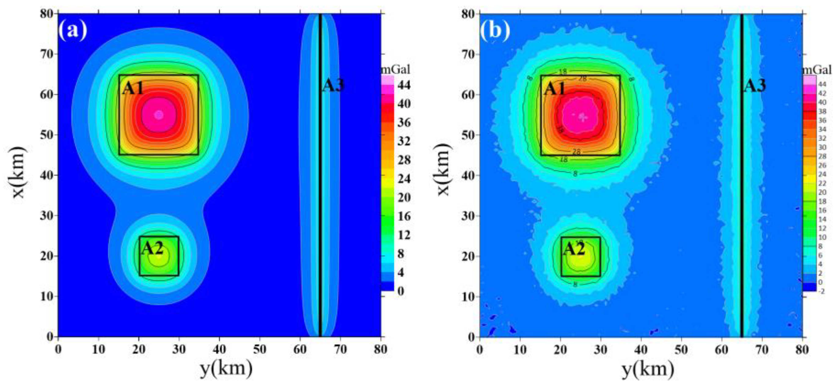
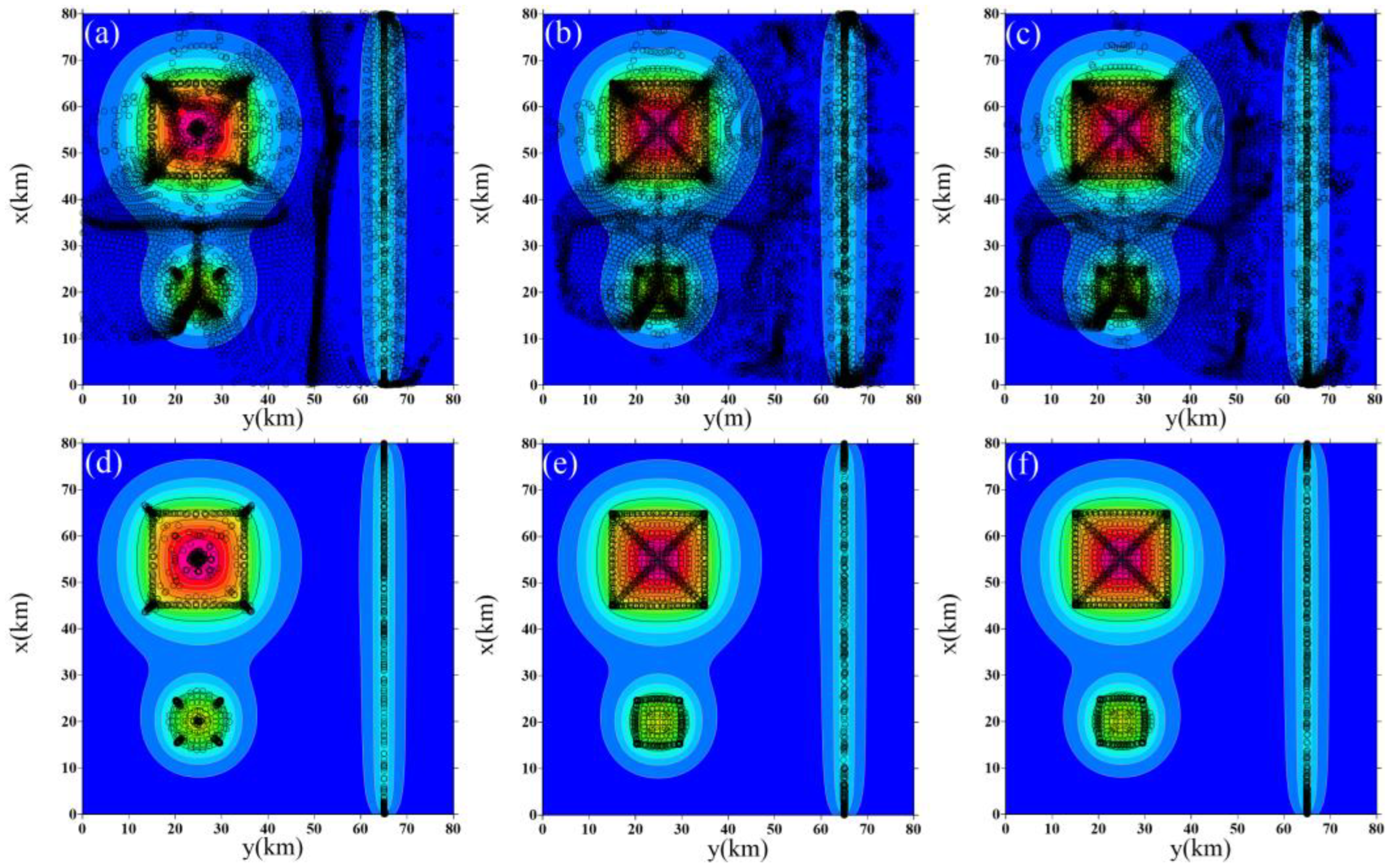
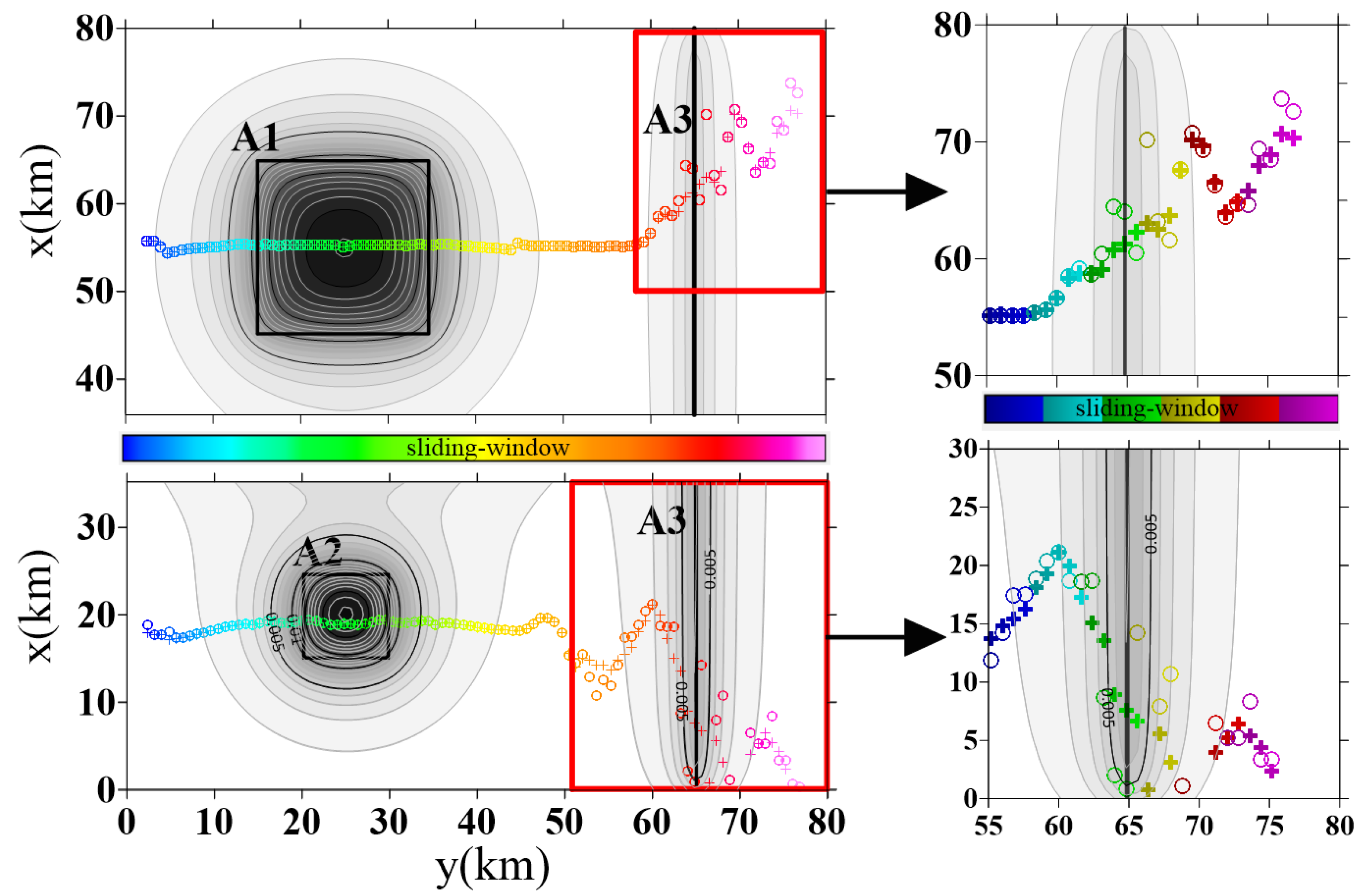
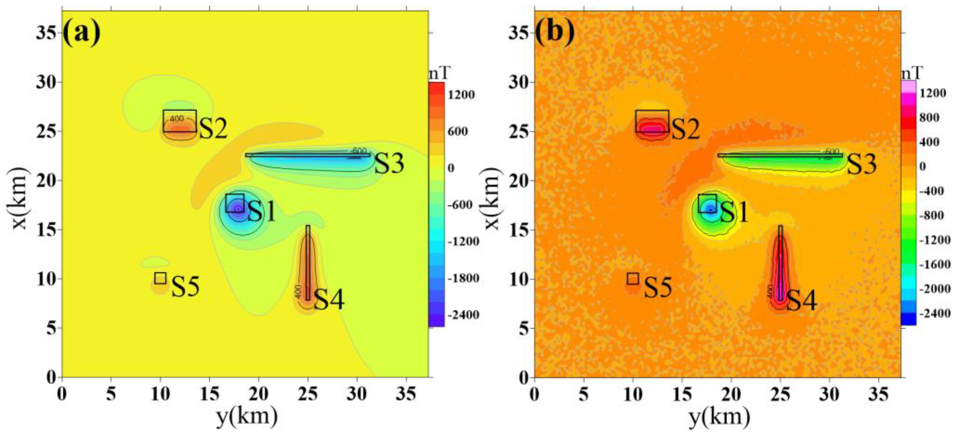
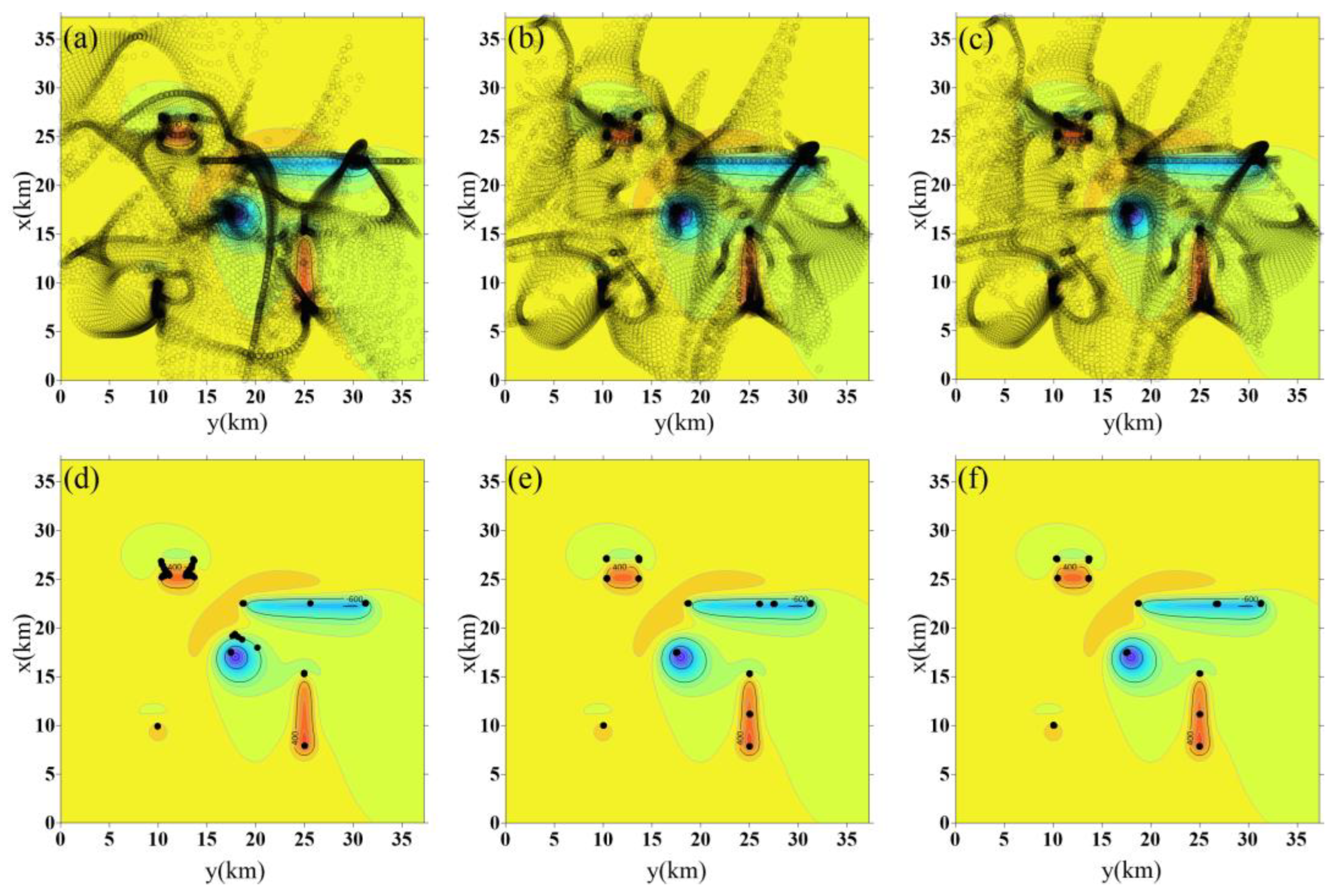
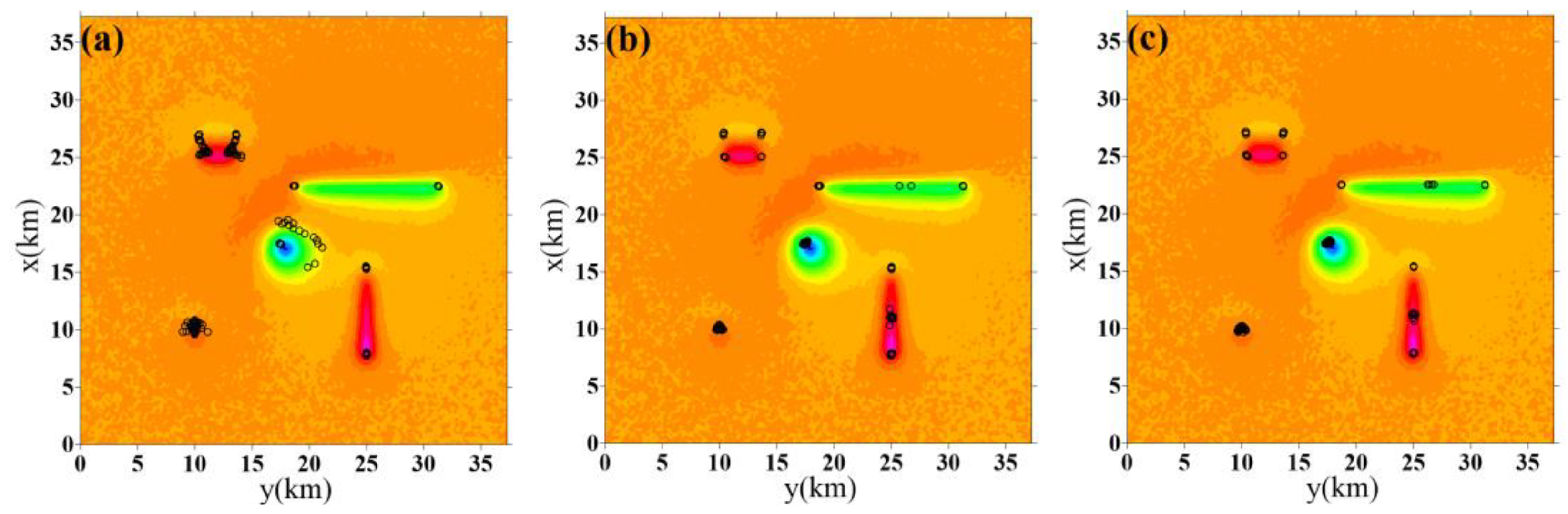
3.4. Test 4: Complex Model Test

This model has been widely used by many authors to test the accuracy of their algorithms [16,18,19,22,26,27,28].

Table 3. Estimated and true coordinates of singular points; 0 represents the true position of the sources, 1 represents the inversion results obtained by our method, and 2 represents the inversion results obtained by the DST algorithm.

Source	x0	x1	x2	y0	y1	y2	z0	z1	z2	N0	N1	N2
S1 sphere	17.5	17.50	17.50	17.5	17.52	17.53	3	3.06	3.04	3	3.11	3.07
S2 sill	25	25.09	25.11	10.5	10.39	10.42	1	0.80	0.85	1	0.69	0.77
	25	25.07	25.09	13.5	13.62	13.60	1	0.82	0.86	1	0.68	0.75
	27	27.12	27.11	13.5	13.65	13.64	1	0.72	0.71	1	0.25	0.25
	27	27.12	27.11	10.5	10.33	10.34	1	0.73	0.72	1	0.25	0.25
S3 Dyke	22.5	22.51	22.51	19	18.72	18.72	1	0.84	0.84	1	1.13	1.13
	22.5	22.50	22.50	31	31.25	31.25	1	0.85	0.85	1	1.13	1.13
S4 Horioz. rod	8	7.88	7.88	25	25.00	25.00	1.5	1.49	1.49	2	2.00	2.00
	15.25	15.32	15.33	25	25.00	25.00	1.5	1.41	1.42	2	1.83	1.84
S5 sphere	10	10.01	10.02	10	10.03	10.03	2	1.97	1.95	3	2.92	2.91

shows the parameters of the model, and Figure 10a shows the model location and the magnetic anomaly. Models S2, S4, and S5 are normally magnetized along the direction of the ambient field (D = 2.4°, I = 59°). Models S1 and S3 are reversely magnetized. In this test, for different algorithms, solutions were calculated using a window size of 11 × 11 (2.75 × 2.75 km) grids. To obtain reliable solutions, we accept solutions according to the following criteria: If the horizontal gradient in the window center is larger than the mean value of the horizontal gradient [29], if the estimated depth lies between 0 km and 3.5 km, if the estimated SI is between 0 and 3, and if the distance between THE two solutions obtained from THE adjacent windows is less than the grid interval.

Figure 11a–c shows the original Euler solutions generated by finite-difference Euler deconvolution, improved finite-difference Euler deconvolution, and Euler deconvolution based on DST, respectively. Figure 11d–f shows the Euler solutions after selection based on the above strategy. Comparing Figure 11a and Figure 11b, we can find that the horizontal distributions of the estimated solutions generated from the two methods are different. Additionally, by analyzing the selected Euler solutions (Figure 11d,e), we find that the selected solutions generated by our method are more helpful to locate the source positions.

Comparing Figure 11b,c, we can find that the horizontal distribution of the original position estimates is almost the same. In Figure 11b,c, the mean values of all the x_0-estimate are 18.71 and 18.63, the mean values of all the y_0-estimate values are 17.12 and 17.06, and the mean values of the z_0-estimate are 1.497 and 1.503, respectively. Additionally, the difference between the mean value is less than the grid interval. To compare the precision of our method and that of Euler deconvolution based on DST, two profiles are selected. Figure 12 shows that the inversion results are nearly consistent. Table 3 shows the final estimated solutions, and by comparing them, we find that the results obtained from our algorithm are almost the same as those of Euler deconvolution based on DST. Based on the results of this model, we find that the precision of our algorithm and of Euler deconvolution based on DST is nearly the same.

Noisy Data

Figure 10b shows the noise-corrupted total-field anomaly data; the theoretical anomaly is corrupted with (2%) random Gaussian noise. Figure 13 shows the results of the Euler deconvolution methods. Based on the results, we find that there are some spurious solutions in Figure 13a, and the estimated horizontal solutions shown in Figure 13b,c are consistent with the horizontal coordinates of singular points of the source. In addition, according to the results of tests 1–3, we find that comparing the solutions generated by finite-difference Euler deconvolution and Euler deconvolution based on DST, the resolution of the results obtained by our method is higher than that of the former and is the same as that of the latter.

Compared with other inversion methods, Euler deconvolution is not a time-consuming method because of the use of the sliding window strategy. However, for large-scale potential field exploration, the data to be inverted are large, and improving the processing speed is good for real-time viewing and interpreting Euler solutions, especially when different SIs and sliding window sizes are needed to obtain useful solutions. We resampled the data shown in Figure 10a and the grid interval is 2, 1/2, 1/4, and 1/6 times the original grid interval. Figure 14 shows the time spent in each inversion process. The result shows that the processing speed of Euler deconvolution based on DST is high, and that our method can take less time to accomplish the deconvolution.

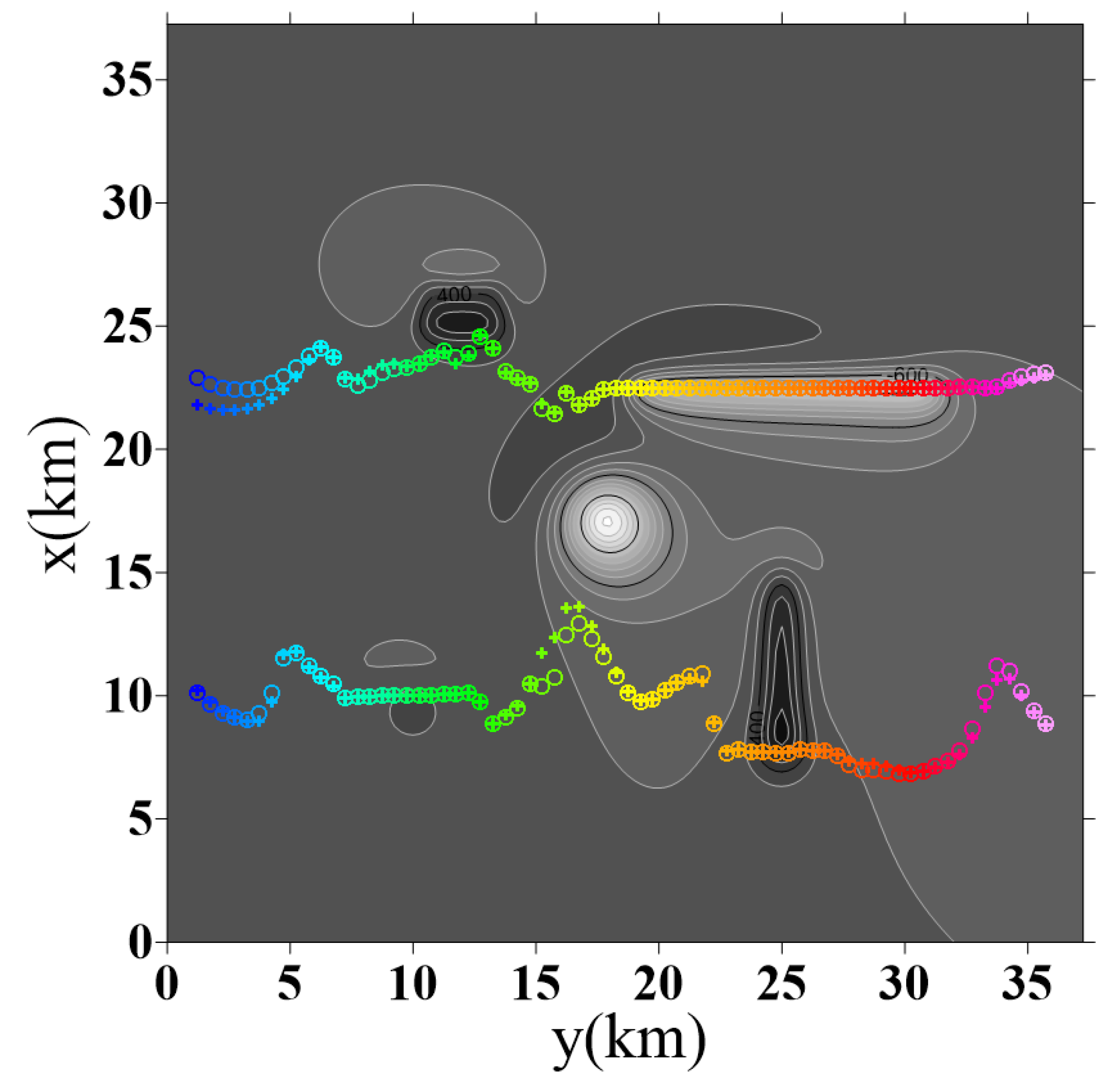
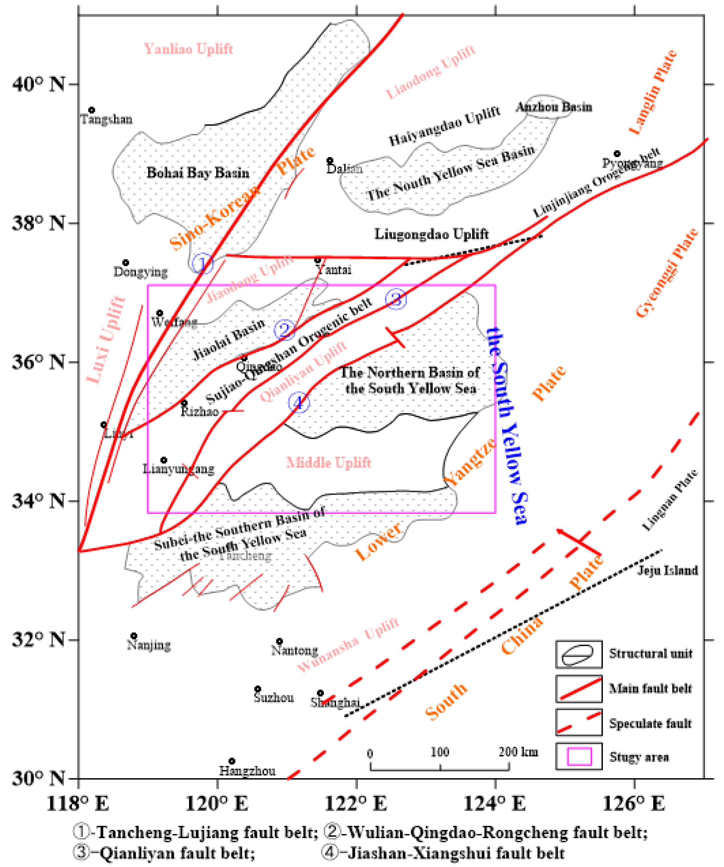
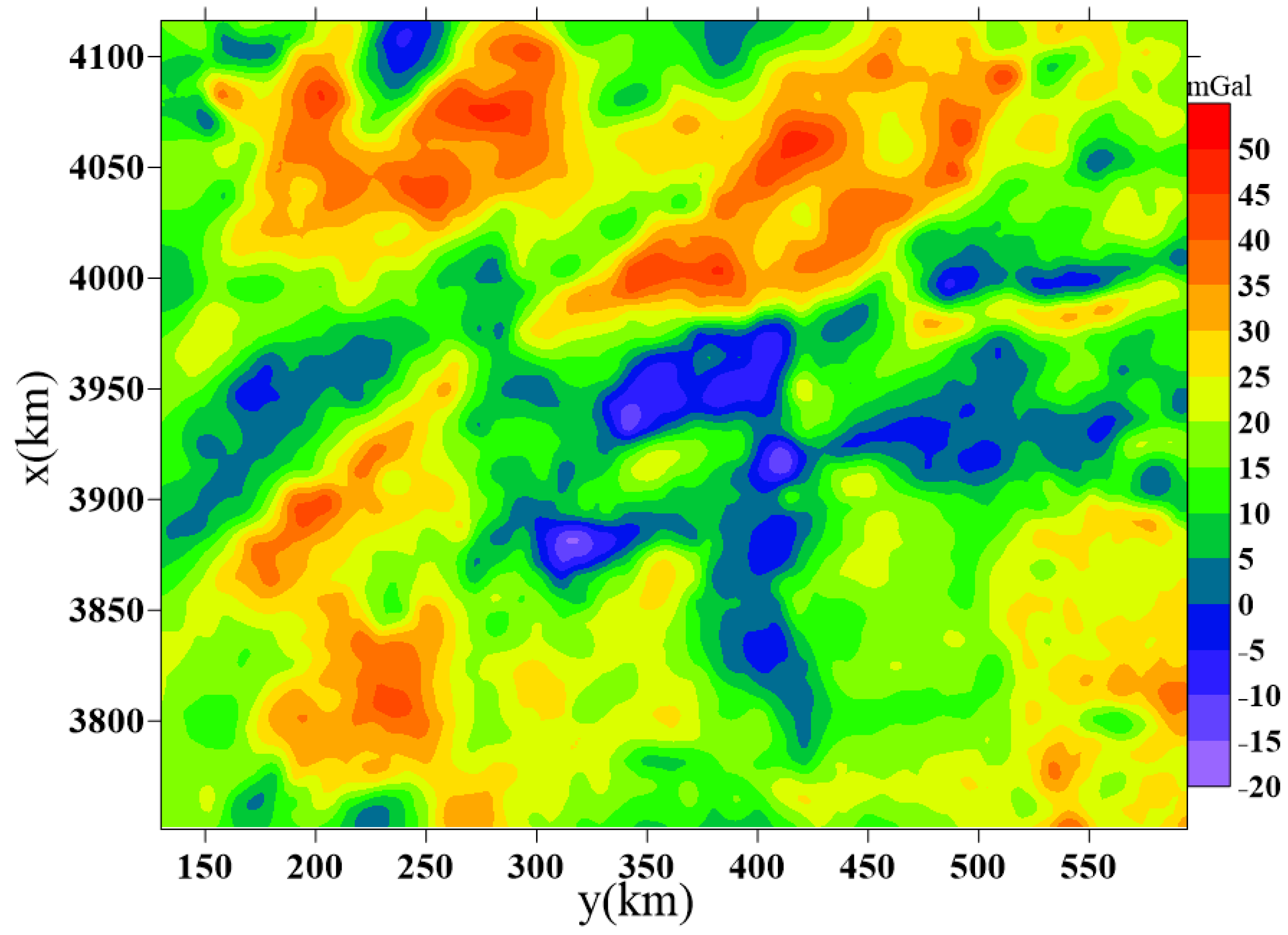
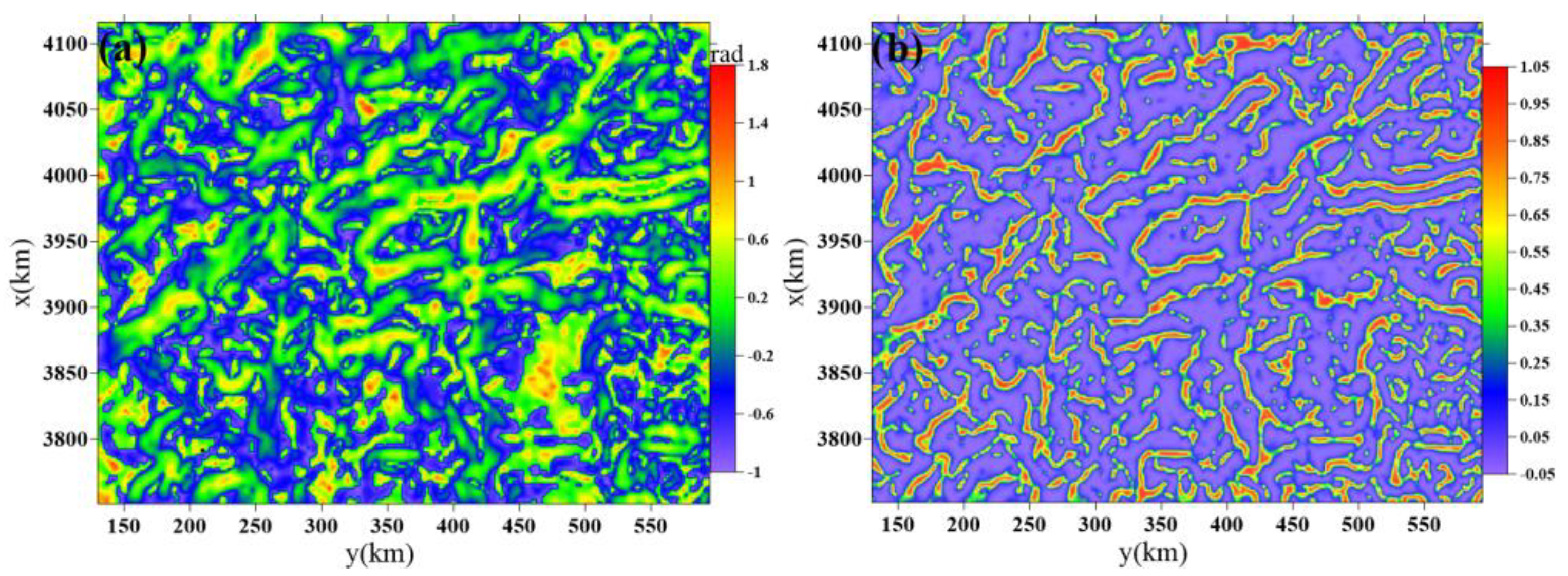
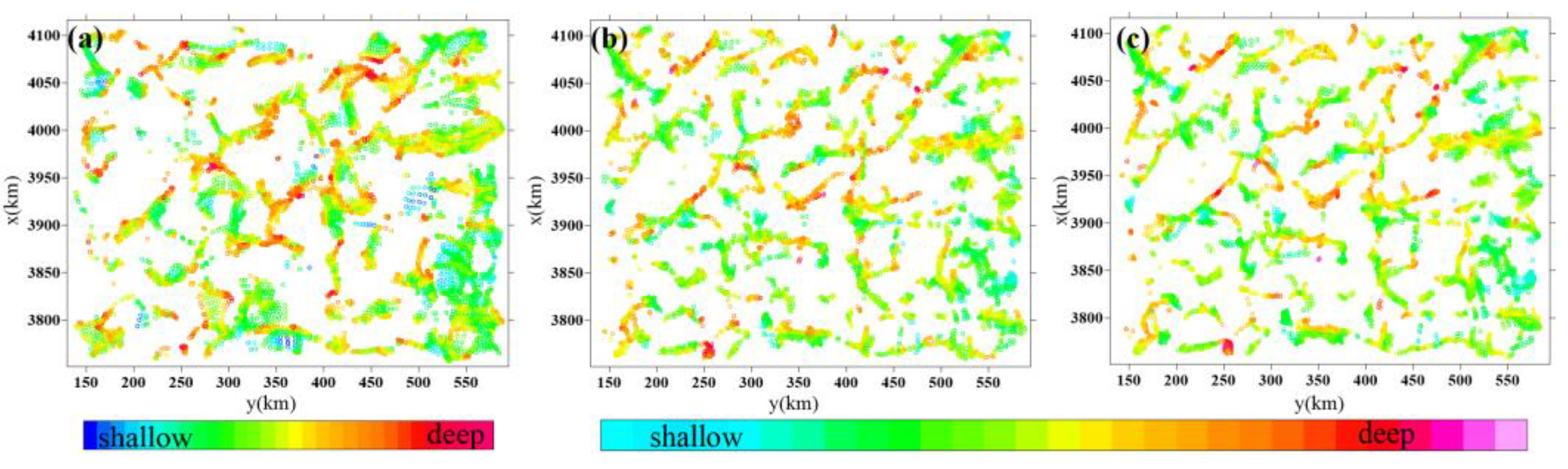
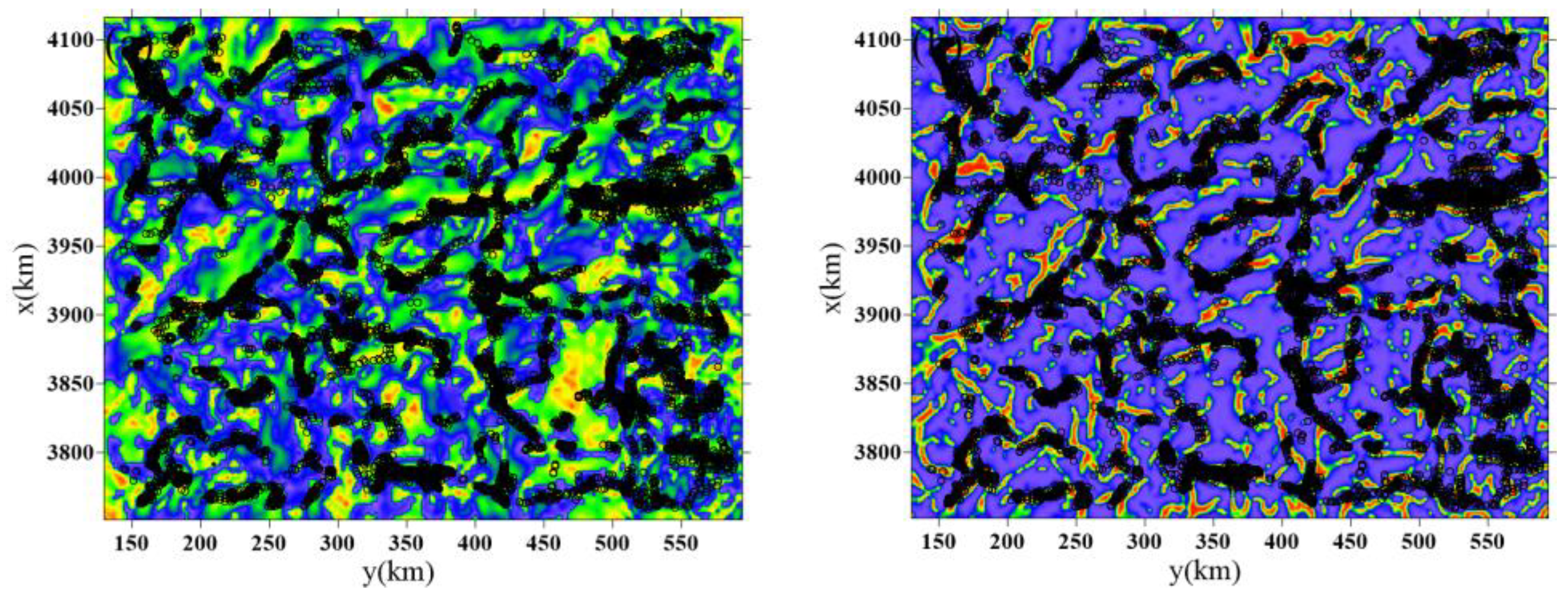
4. Application to Real Data

The study area (Figure 15), which straddles three major tectonic units, the Sino-Korean, Yangzi, and South China plates, underwent the consolidated diagenesis and reactivation of the Late Sibao Movement in the Mesoproterozoic Era and of the Jinning Movement in the Neoproterozoic Era, forming a two-layer crystalline basement of Meso-Neoproterozoic shallow metamorphic rock and Archean-Paleoproterozoic deep metamorphic rock [30,31,32]. Under the influence of the multi-period tectonic movement reformations and the action of various tectonic stresses, the study area has successively experienced tectonic activities of various natures, such as extensional fault depressions, and strike-slip subsidence [33]. It is a marine-continent multi-cycle superimposed petroliferous basin that has been formed based on the pre-Sinian metamorphic basement.

Based on the collected density information about the study area [34,35], vertically, the density decreases gradually from deep to shallow; horizontally, the density of different tectonic units varies. This density difference facilitates our use of gravity data to study the tectonic distribution of the zone. Figure 16 shows the Bouguer gravity map of the region.

Next, we apply the enhanced total horizontal derivative, improved logistic filter (IL, [36]), and the Euler deconvolution method to the gravity data in this area. The IL is based on the logistic function and the horizontal gradient amplitude and outlines the source horizontal boundaries more clearly and with high accuracy and resolution. Figure 17a is the enhanced total horizontal derivative of the data in Figure 16, and Figure 17b shows the IL. Figure 18 shows the final Euler solutions. Before performing Euler deconvolution, the selected sliding window size is 11 × 11 (22 × 22 km), and the SI is 1.5. The same distinguishing method is applied to select the results generated by the three Euler algorithms, and the Euler solutions with a small standard error of estimated depth (top 30%) are saved.

In Figure 18, the depth of the solution is indicated by the color, so we do not ascribe much accuracy to these depths and prefer to use the descriptors ‘shallow’ and ‘deep’. By comparing Figure 18a and Figure 18b, we find that the distribution of Euler solutions generated from finite-difference Euler deconvolution and improved finite-difference Euler deconvolution is different, and our algorithm shows more detail. The depth range in Figure 18a is 0.1~21.9 km, and the depth range in Figure 18b is 0.4~22.8 km. By comparing Figure 18b and Figure 18c, we find that the distribution of Euler solutions generated from our method and DST Euler deconvolution is almost the same, including the estimated depth. By comparing the Euler solutions and the edge detection results, we find that their distribution patterns are very similar (Figure 19). Additionally, this fully demonstrates the effectiveness of our method. The distribution of the Euler soluitons and the peaks of the IL present a good correlation with some faults in the region, which are shown by Xu [32].

Based on the stratigraphic distribution, structural trend, geomorphological characteristics, and distribution of magmatic rocks [33], the Euler solutions (NE (NNE)) are consistent with the regional tectonic trend. Additionally, the Euler results indicate that NEE-NE trending faults are distributed throughout the region, with NE-NEE trending faults being predominantly found in the northern basin and northwest areas outside the basin, and near-EW trending faults are mainly present in the central uplift area. These observations are mainly attributed to the influence of Tanlu fault strike–slip activity and its nearby north–south stress control [32,34].

5. Conclusions

In this paper, we present a new method for reducing the influence of background fields on Euler results, called improved finite-difference Euler deconvolution. It is based on the finite-difference method and accounts for a linear background field. We demonstrated our algorithm on synthetic and real potential field data and compared the results with those of finite-difference Euler deconvolution and Euler deconvolution based on DST. The inversion results show that our method can simultaneously estimate the source position, SI, and the coefficient of the linear background field, and that the precision of its results is higher than the results computed by the finite-difference Euler deconvolution method. The inversion results also show that the accuracy of the inversion results is close to that of the results of the DST inversion algorithm, even in the case of strong interference and noise.

References

1. Werner, R.T. Interpretation of Magnetic Anomalies at Sheet-Like Bodies. Sver. Geol. Unders. Ser. C Arsb. 1953, 6, 413–449. [Google Scholar]
2. Hansen, R.O.; Simmonds, M. Multiple-source Werner deconvolution. Geophysics 1993, 58, 1792–1800. [Google Scholar] [CrossRef]
3. Hansen, R.O. 3D multiple-source Werner deconvolution for magnetic data. Geophysics 2005, 70, L45–L51. [Google Scholar] [CrossRef]
4. Thompson, D.T. EULDPH: A new technique for making computer-assisted depth estimates from magnetic data. Geophysics 1982, 47, 31–37. [Google Scholar] [CrossRef]
5. Reid, A.B.; Allsop, J.M.; Granser, H.; Millett, A.T.; Somerton, I.W. Magnetic interpretation in three dimensions using Euler deconvolution. Geophysics 1990, 55, 80–91. [Google Scholar] [CrossRef]
6. Barbosa, V.; Silva, J.B.C.; Medeiros, W.E. Stability analysis and improvement of structural index estimation in Euler deconvolution. Geophysics 1999, 64, 48–60. [Google Scholar] [CrossRef]
7. Stavrev, P.; Reid, A. Degrees of homogeneity of potential fields and structural indices of Euler deconvolution. Geophysics 2007, 72, L1–L12. [Google Scholar] [CrossRef]
8. Nabighian, M.N. The analytic signal of two-dimensional magnetic bodies with polygonal cross-section: Its properties and use for automated anomaly interpretation. Geophysics 1972, 37, 507–517. [Google Scholar] [CrossRef]
9. Nabighian, M.N. Additional comments on the analytic signal of two-dimensional magnetic bodies with polygonal cross-section. Geophysics 1974, 39, 85–92. [Google Scholar] [CrossRef]
10. Nabighian, M.N. Toward a three-dimensional automatic interpretation of potential field data via generalized Hilbert transforms: Fundamental relations. Geophysics 1984, 49, 780–786. [Google Scholar] [CrossRef]
11. Bastani, M.; Pedersen, L.B. Automatic interpretation of magnetic dike parameters using the analytical signal technique. Geophysics 2001, 66, 551–561. [Google Scholar] [CrossRef]
12. Fedi, M. DEXP: A fast method to determine the depth and the structural index of potential fields sources. Geophysics 2007, 72, I1–I11. [Google Scholar] [CrossRef]
13. Abbas, M.A.; Fedi, M. Automatic DEXP imaging of potential fields independent of the structural index. Geophys. J. Int. 2014, 199, 1625–1632. [Google Scholar] [CrossRef]
14. Hsu, S.-K. Imaging magnetic sources using Euler’s equation. Geophys. Prospect. 2002, 50, 15–25. [Google Scholar] [CrossRef]
15. Nabighian, M.N.; Hansen, R.O. Unification of Euler and Werner deconvolution in three dimensions via the generalized Hilbert transform. Geophysics 2001, 66, 1805–1810. [Google Scholar] [CrossRef]
16. Gerovska, D.; Stavrev, P.; Araúzo-Bravo, M. Finite-difference Euler Deconvolution Algorithm Applied to the Interpretation of Magnetic Data from Northern Bulgaria. Pure Appl. Geophys. 2005, 162, 591–608. [Google Scholar] [CrossRef]
17. Stavrev, P.Y. Euler deconvolution using differential similarity transformations of gravity or magnetic anomalies. Geophys. Prospect. 1997, 45, 207–246. [Google Scholar] [CrossRef]
18. Gerovska, D.; Araúzo-Bravo, M.J.; Stavrev, P.; Whaler, K. MaGSoundDST—3D automatic inversion of magnetic and gravity data based on the differential similarity transform. Geophysics 2010, 75, L25–L38. [Google Scholar] [CrossRef]
19. Gerovska, D.; Araúzo-Bravo, M.J.; Whaler, K.; Stavrev, P.; Reid, A. Three-dimensional interpretation of magnetic and gravity anomalies using the finite-difference similarity transform. Geophysics 2010, 75, L79–L90. [Google Scholar] [CrossRef]
20. Gerovska, D.; Arauzo-Bravo, M.J.; Whaler, K. A Comparison of Three Automatic Interpretation Techniques for Magnetic and Gravity Data. In Proceedings of the 72nd EAGE Conference and Exhibition Incorporating SPE EUROPEC 2010, Barcelona, Spain, 14–17 June 2010; p. 161-00120. [Google Scholar]
21. Pasteka, R. The role of the interference polynomial in the Euler deconvolution algorithm. Boll. Geofis. Teor. Appl. 2006, 47, 171–180. [Google Scholar]
22. Dewangan, P.; Ramprasad, T.; Ramana, M.V.; Desa, M.; Shailaja, B. Automatic Interpretation of Magnetic Data Using Euler Deconvolution with Nonlinear Background. Pure Appl. Geophys. 2007, 164, 2359–2372. [Google Scholar] [CrossRef]
23. Reid, A.B.; Ebbing, J.; Webb, S.J. Avoidable Euler Errors-the use and abuse of Euler deconvolution applied to potential fields. Geophys. Prospect. 2014, 62, 1162–1168. [Google Scholar] [CrossRef]
24. Cooper, G. Obtaining dip and susceptibility information from Euler deconvolution using the Hough transform. Comput. Geosci. 2006, 32, 1592–1599. [Google Scholar] [CrossRef]
25. Liu, Q.; Yao, C.; Zheng, Y. Euler deconvolution of potential field based on damped least square method. Chin. J. Geophys. 2019, 62, 3710–3722. (In Chinese) [Google Scholar] [CrossRef]
26. Qiang, L.; Changli, Y.; Yao, L.; Junjun, Y.; Zelin, L. Euler solution selecting method based on the damping factor. Acta Geophys. 2022, 70, 1551–1564. [Google Scholar] [CrossRef]
27. Wang, J.; Meng, X.; Li, F. New improvements for lineaments study of gravity data with improved Euler inversion and phase congruency of the field data. J. Appl. Geophys. 2017, 136, 326–334. [Google Scholar] [CrossRef]
28. Gerovska, D.; Araúzo-Bravo, M.J. Automatic interpretation of magnetic data based on Euler deconvolution with unprescribed structural index. Comput. Geosci. 2003, 29, 949–960. [Google Scholar] [CrossRef]
29. Yao, C.L.; Guan, Z.N.; Wu, Q.B.; Zhang, Y.W.; Liu, H.J. An analysis of Euler deconvolution and its improvement. Geophys. Geochem. Explor. 2004, 28, 150–155. [Google Scholar]
30. Wang, L.W. Basic characteristics of geology and prospects of oil andgas production in the Southern Huanghai Sea basin. Mar. Geol. Quat. Geol. 1989, 9, 41–50. [Google Scholar]
31. Cai, Q.Z. Oil & Gas Geology in China Seas; Ocean Press: Beijing, China, 2005. [Google Scholar]
32. Li, J.B. Regional Oceanography of China Seas Marine Geology; Ocean Press: Beijing, China, 2012. [Google Scholar]
33. Xu, W.Q.; Yuan, B.Q.; Liu, B.L.; Yao, C.L. Multiple gravity and magnetic potential field edge detection methods and their application to the boundary of fault structures in northern South Yellow Sea. Geophys. Geochem. Explor. 2020, 44, 962–974. [Google Scholar] [CrossRef]
34. Wanyin, W.; Jinlan, L.; Zhiyun, Q.; Yijian, H.; Dongsheng, C. A research on Mesozoic thickness using satellite gravity anomaly in the southern Yellow Sea. China Offshore Oil Gas 2004, 16, 151–156. [Google Scholar]
35. Yao, C.L. Research of Gravity-Magnetic-Seismic Integrated Inversion Technology and Processing &Interpretation of Gravity and Magnetic Data in the Yellow Sea and Adjacent Regions; China University of Geosciences: Beijing, China, 2005. [Google Scholar]
36. Pham, L.T.; Van Vu, T.; Le Thi, S.; Trinh, P.T. Enhancement of Potential Field Source Boundaries Using an Improved Logistic Filter. Pure Appl. Geophys. 2020, 177, 5237–5249. [Google Scholar] [CrossRef]
Figure 1. Synthetic magnetic profile and Euler solutions. (a) Synthetic magnetic profile generated by two dykes shown in Figure 1b below (red lines). (b) Original Euler solutions generated by finite-difference Euler deconvolution. (c) Priginal Euler solutions generated by the improved method. (d,e) The selected solutions from (b,c); solutions are selected according to the moving-rate selection method.
Applsci 13 05323 g001
Figure 2. Noise-corrupted synthetic magnetic profile and Euler solutions. (a) Synthetic magnetic profile generated by two dykes (red lines in Figure 2), corrupted with 0.5% random Gaussian noise shown in Figure 2b below. (b) Original Euler solutions generated by finite-difference Euler deconvolution. (c) Original Euler solutions generated by the improved method. (d,e) Selected solutions from (b,c); solutions are selected according to the moving-rate selection method.
Applsci 13 05323 g002
Figure 3. Synthetic anomaly data. (a) Linear background. (b) Theoretical gravity anomaly generated by a prism (black line represents the field source boundary). (c) Synthetic anomaly (a + b). (d) Synthetic anomaly corrupted with 1% Gaussian random noise.
Applsci 13 05323 g003
Figure 4. Euler solutions. (ac) Original Euler solutions generated by the finite-difference Euler deconvolution, our method, and the DST method. Solutions are saved if the vertical derivative of gravity of the window center is not negative. (df) Selected Euler solutions.
Applsci 13 05323 g004
Figure 5. Euler solutions obtained from the noise-corrupted model. (ac) Original Euler solutions generated by finite-difference Euler deconvolution, our method, and the DST method. Solutions are saved if the vertical derivative of gravity of the window center is not negative. (df) Selected Euler solutions.
Applsci 13 05323 g005
Figure 6. True location of synthetic prisms (the black rectangles) and the gravity anomaly produced by them. (a) Theoretical gravity anomaly. (b) Theoretical gravity anomaly corrupted with 2% Gaussian random noise.
Applsci 13 05323 g006
Figure 7. Original and selected Euler solutions (The base map shows the distribution of magnetic anomalies). (a) Original Euler solutions generated by finite-difference Euler deconvolution. (b) Original Euler solutions generated by improved finite-difference Euler deconvolution. (c) Priginal Euler solutions generated by the euler deconvolution based on DST. (df) Solutions distinguished from (ac); Solutions are saved if the vertical derivative of gravity of the window center is positive.
Applsci 13 05323 g007
Figure 8. Two profiles are selected for inversion, different colors represent different window positions. + represents the solutions obtained by DST. ○ represents the solutions obtained by our method.
Applsci 13 05323 g008
Figure 9. Original and selected Euler solutions (The base map shows the distribution of magnetic anomalies). (a) Original Euler solutions generated by finite-difference Euler deconvolution. (b) Original Euler solutions generated by improved finite-difference Euler deconvolution. (c) Original Euler solutions generated by Euler deconvolution based on DST. (df) Solutions distinguished from (ac).
Applsci 13 05323 g009
Figure 10. Model location and the magnetic anomaly generated by the five models. (a) Noise-free total-field anomaly. (b) Noise-corrupted total-field anomaly (2% random Gaussian noise). Table 3 shows the details of the model.
Applsci 13 05323 g010
Figure 11. Distributions of the Euler solutions obtained from the three algorithms (The base map shows the distribution of magnetic anomalies). (a) Finite-difference Euler deconvolution algorithm. (b) Our algorithm. (c) DST Euler deconvolution algorithm. (df) Solutions after distinguished from (ac), and the selection method is described in the previous paragraph above Figure 6.
Applsci 13 05323 g011
Figure 12. Inversion results from two profiles; different colors represent different window positions. + represents the solutions obtained by DST. ○ represents the solutions obtained by our method.
Applsci 13 05323 g012
Figure 13. Filtered Euler solutions from different algorithms (The base map shows the distribution of magnetic anomalies). (a) Finite-difference Euler deconvolution algorithm. (b) Our algorithm. (c) Euler deconvolution algorithm based on DST.
Applsci 13 05323 g013
Figure 14. Time spent in each inversion process. Circles of different colors represent different mesh sizes.
Applsci 13 05323 g014
Figure 15. Sketch map of the tectonic location of the northern basin of the south of the Yellow Sea and its adjacent area (modified from Xu [30]).
Applsci 13 05323 g015
Figure 16. The Bouguer gravity map of the study area.
Applsci 13 05323 g016
Figure 17. Edge recognition results. (a) Enhanced total horizontal derivative. (b) IL (unitless).
Applsci 13 05323 g017
Figure 18. Results of Euler deconvolution. (a) Final Euler solutions generated by finite-difference Euler deconvolution. (b) Final Euler solutions generated by improved finite-difference Euler deconvolution. (c) Final Euler solutions generated by Euler deconvolution based on DST.
Applsci 13 05323 g018
Figure 19. Edge recognition results and the Euler solutions generated by our method. (a) Figure 17a + Figure 18b. (b) Figure 17b + Figure 18b.
Applsci 13 05323 g019