Article

Machine Learning for Short-Term Prediction of Ship Motion Combined with Wave Input

1
Marine Design & Research Institute of China, Shanghai 200011, China
2
China State Shipbuilding Corporation Limited, Shanghai 200011, China
*
Author to whom correspondence should be addressed.
Appl. Sci. 2023, 13(9), 5298; https://doi.org/10.3390/app13095298
Submission received: 25 February 2023 / Revised: 18 March 2023 / Accepted: 21 April 2023 / Published: 24 April 2023
(This article belongs to the Special Issue Advances in Nautical Engineering and Maritime Transport)

Abstract

:
There is a response relationship between wave and ship motion. Based on the LSTM neural network, the mapping relationship between the wave elevation and ship roll motion is established. The wave elevation and ship motion duration data obtained by the CFD simulation are used to predict ship roll motion with different input data schemes. The results show that the prediction scheme considering the wave elevation input can predict ship roll motion. Compared with the direct prediction scheme based on the roll data input, the prediction scheme considering the wave elevation input factor can greatly improve the prediction accuracy and effective advance prediction time. Different wave elevation data inputs have different prediction effects. The advance prediction duration will increase with the increase in the input wave elevation position and the ship distance. The simultaneous input of multi-point wave elevation greatly increases the amount of data, allowing the trained model to utilize a greater data depth. This not only improves the advance prediction duration of the prediction model, but it also enhances the robustness of the model, making the prediction results more stable.

1. Introduction

Ships present random motion under the action of irregular waves. The violent motion of ships harms their navigation and operation. Wave is the main incentive factor of the ship oscillation motion. If the mapping relationship between wave elevation near the ship and ship motion can be established, the ship motion can be predicted in a very short time. Its motion attitude for a period of time in the future can be known in advance, so as to ensure the safety of the ship’s operation at sea.
The very short-term prediction of ship motion refers to the prediction of a ship’s motion in the next few seconds to tens of seconds. Triantafyllou and Bodson (1983) [1] used the Kalman filter (KF) method to study the very short-term prediction of the ship motion. Through the characteristics of the ship motion and the corresponding assumptions, the mechanical principle was used to analyze the force on the ship. The state equation of the ship sway motion was derived, so as to obtain the multi-step ship motion predictor based on the KF method. The KF method needs an accurate ship motion state equation. Because the sea state environment often changes, the hydrodynamic parameters are not stable enough, which makes it difficult to obtain an accurate ship motion state equation. Zhao et al. (2004) [2] used minor component analysis (MCA) to predict ship motion a long time ahead with consistent accuracy. The prediction error is almost the same for the 5 s and 20 s predictions. Li et al. (2017) [3] used a nonlinear autoregressive exogenous (NARX) network combining 29 ship state attributes to predict heading, roll, and pitch. Their study showed that modeling and analyzing based on the NARX network was helpful in generating the data-driven model for the ship motion prediction. Suhermi et al. (2018) [4] combined the depth neural network (DNN) and the auto-regressive (AR) model to predict the ship roll data. The results show that the mixed model has better prediction accuracy than the single depth feedforward neural network and AR model. Duan et al. (2015) [5] developed a novel order selection approach based on ship impulse response function (IRF). Additionally, the AR model using the IRF order selection is designated as an IRF-AR model. The simulation results of an S175 container ship showed the superiority of the IRF-AR model to the conventional model in prediction accuracy, efficiency, and algorithm adaptation. Yin et al. (2018) [6] established an ensemble mechanism by combining the discrete wavelet transform and variable radial basis function (RBF) networks. The effectiveness of the proposed discrete wavelet transform (DWT)-based real-time roll prediction scheme was demonstrated by short-term ship roll motion prediction experiments based on the actual ship roll motion measurements collected. Li and Hong (2019) [7] optimized the least squares support vector regression (SVR) model through the chaotic cloud particle swarm optimization algorithm and combined it with the periodogram estimation method. They developed this hybrid model algorithm for predicting ship motion and carried out prediction analysis with two sets of real ship data. The results show that the hybrid model has better prediction accuracy than the classical prediction model. Based on the SVR, Duan et al. (2015) [8] proposed a hybrid model for forecasting the nonlinear and non-stationary short-term prediction of ship motion. The difficulty of processing non-stationary data in the SVR model was overcome by using the mode decomposition (EMD) technology, which has higher accuracy for the very short-term prediction results of the ship motion.
In recent years, the artificial neural network has been widely used in the ship motion prediction. The cyclic neural network is a kind of time recursive neural network that can process the information of sequence structure. Shen (2005) [9] established a diagonal recurrent neural network (RNN) model for large ship motion prediction. The results were compared with the AR prediction method and the periodogram prediction method. The prediction results show the feasibility of the algorithm.
The long short-term memory (LSTM) neural network [10] is a special cyclic neural network. Its special gating structure makes it have the ability of long-term memory and can process time series data more effectively. Wang et al. (2017) [11] used the LSTM neural network and traditional RNN and AR models to carry out a comparative analysis of ship motion prediction, proving that the LSTM neural network has better prediction accuracy. D’Agostino et al. (2021) [12] assessed and compared the performance of RNN, LSTM, and gated recurrent units (GRU) models using a data set obtained from computational fluid dynamics (CFD) simulations of a self-propelled destroyer-type vessel. The objective was to obtain about a prediction of 20 s ahead. The three methods provided promising and comparable results.
Zhang et al. (2019) [13] carried out prediction research on USV roll data by combining the convolution neural network (CNN) and LSTM neural network. The results proved that the combined prediction model has better a prediction effect. The EMD-LSTM combined forecasting model established by Zhang et al. (2020) [14] has better forecasting accuracy than the single LSTM model. Peng et al. (2019) [15] integrated the particle swarm optimization algorithm (PSO) and the EMD algorithm on the LSTM neural network algorithm. The results show that the hybrid model can effectively improve the prediction accuracy. Geng et al. (2023) [16] proposed a prediction algorithm based on EMD and adaptive PSO-LSTM with the sliding window approach. The simulation results demonstrate that the proposed model performs well in terms of predicting the nonlinear and nonstationary ship roll and pitch. Zhang et al. (2021) [17] combined an attention mechanism (AM) with LSTM, and carried out prediction tests using real ship data. The results show that this method has better prediction performance than other common methods. Sun et al. (2022) [18] used the LSTM neural network and Gaussian process regression (GPR) to predict the ship rolling angle and pitch angle. The model yielded reliable interval prediction results without reducing the forecasting accuracy of the LSTM model, which verified the effectiveness and advancement of the hybrid model. Wang et al. (2021) [19] proposed a ship roll angle prediction method based on the bidirectional long short-term memory network (BLSTM) and temporal pattern attention mechanism (TPA). Compared with the LSTM model and the SVM model, the combined model had a significant reduction in errors. Later, Wang et al. (2021) [20] proposed the single input single output (SISO) and multiple input single output (MISO) methods to predict ship motion based on deep learning. The methods achieved good prediction accuracy. Table 1 summarizes the relevant machine learning models for the short-term perdition of ship motion.
At present, most scholars used the LSTM neural network to predict ship motion in the very short-term, mostly based on the data of ship motion itself, while there are few reports on the research of ship motion prediction based on wave elevation data. In fact, in the process of ship operation at sea, especially at zero speed, waves are the main excitation of ship movement. The wave itself has the memory effect. If the ship movement can be predicted in the very short-term by using the wave elevation data as the input feature, the prediction duration and prediction accuracy can be effectively improved in theory. In order to verify the effectiveness of the scheme, this paper, based on the LSTM neural network model, combined with wave elevation and ship motion duration data to study the very short-term prediction of ship roll motion.

2. LSTM for Ship Motion Prediction

2.1. LSTM Theory

The LSTM unit structure is composed of the forgetting gate, input gate, output gate, and unit state. The unit structure is shown in Figure 1. At the current time t, there are three input parameters of the LSTM network: input value xt at the current time (such as wave elevation), output value ht−1 at the previous time (such as roll motion), and unit state Ct−1 at the previous time. There are two output parameters: the current time output value ht and the current time unit state Ct. Through the activation function σ, the LSTM realizes the control of the three gates, so as to preserve and forget the historical information. Referring to study [21] for the specific principle of the mathematical expression of the gating structure.
The function of forgetting gate determines how many Ct−1 unit states need to be retained until the current moment. The mathematical expression is as follows:
f t = σ ( W f [ h t 1 , x t ] + b f )
where Wf is the vector weight; bf is the offset vector quantity. The gate will read the two input values, xt and ht−1, and activate the function σ (sigmoid function) that controls the output of a value between 0 and 1 to Ct−1, where 0 represents the complete rejection of Ct−1 and 1 represents the complete retention of Ct−1.
The function of the input gate determines how much new data need to be saved to the cell state Ct. The mathematical expression is as follows:
i t = σ ( W i [ h t 1 , x t ] + b i )
C ˜ t = tanh ( W c [ h t 1 , x t ] + b c )
C t = f t C t 1 + i t C ˜ t
The gate needs two steps to realize the new unit state Ct. The first step is to determine which information needs to be updated through Equation (2), and calculate the temporary state at the current time through Equation (3). The second step is to obtain the new unit state Ct at the current time through Equation (4).
The function of the output gate controls how much of the unit state Ct needs to be output to ht. The mathematical expression is as follows:
o t = σ ( W o [ h t 1 , x t ] + b o )
h t = o t tanh ( C t )
The door activates the function through Equation (5) σ to determine the output part ot in the cell state Ct, and then determine the final output value ht through Equation (6).

2.2. LSTM Theory

The main process of the ship motion prediction model based on the LSTM neural network includes data preprocessing, model parameter setting, model training, prediction data, and prediction result evaluation.
Normalization can reduce the impact of the data magnitude differences, accelerate convergence speed, and improve computational efficiency. All data in this study are normalized first, and then LSTM training is conducted. After the prediction, the data are restored by anti-normalization processing. The normalization method is expressed as follows:
x = x x min x max x min
where x* is the normalized value of x; xmax and xmin represent the maximum and minimum values of x, respectively.
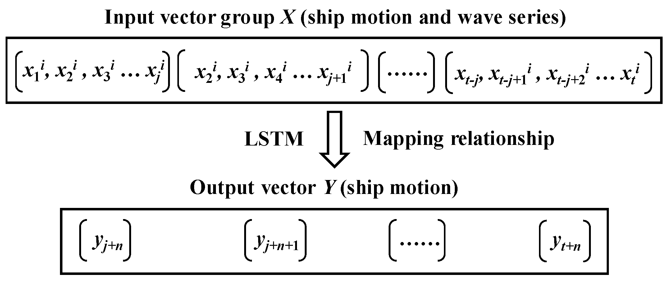
The LSTM neural network can realize a multi-feature input, as shown in Figure 2. When training, it is necessary to establish the mapping relationship between the input duration data xti and the output duration data yt; where i represents the number of input feature types. First, the input duration data group is slided to form the input vector group X. The window length j is the number of input steps. The output vector group Y is the output data yj+n corresponding to each window, where n is the number of advance prediction steps and is used to control the advance prediction duration. The advance prediction duration is n times the sample data sampling interval. The wave elevation input data are used to predict the ship motion. When n = 1, the prediction model predicts the ship motion attitude at the current time. When n > 1, the prediction model predicts the ship motion attitude corresponding to the n-th data moment in the future. The maximum absolute error (MAE) and the root mean square error (RMSE) are used to evaluate the forecast results. The MAE represents the error of the data peak point, while the RMSE represents the overall prediction error.

3. Ship Motion Data

In this study, the motion of ships in irregular waves is simulated by the CFD method. The time-history data of the ship motion and wave elevation at different positions on the ship’s side are obtained for the study of the short-term prediction of ship motion. The test ship is DTMB5415 with scale ratio of 1/51. The ship parameters are listed in Table 2. The simulated working condition is the roll and heave motion of the ship with zero speed in the beam wave sea state of level five. The sea wave spectrum adopts the Pierson–Moskowitz spectrum. The significant wave height at the model scale is 0.078 m. The average wave period is 0.98 s.
The CFD solver is STAR-CCM+. The computation model is based on solving the Reynolds time-averaged Navier–Stokes (RANS) equation combined with the shear stress transport (SST) k-ω formulation. The interface of water and air is captured using the volume of the fluid method with a second-order high resolution interface capturing (HRIC) scheme. The mesh updates caused by the ship motion are processed using the dynamic overlapping mesh technology. An irregular wave is generated through the velocity entry boundary condition. A damping source method is used to eliminate the reflection of waves from the open boundary. The time stepping method is a second-order implicit scheme. The algorithm of the semi-implicit method for pressure-linked equations (SIMPLE) is used to couple the pressure and velocity fields. The computational grid is generated by the trimmer mesher. The boundary layer of the hull surface is divided by a prism layer grid. The thickness of the first layer of the grid adjacent to the hull surface is 2 mm, to ensure that the Y+ value on the ship’s wetted surface is within 100. In order to ensure the accuracy of the wave surface generation and propagation, the grid in the vicinity of the wave surface is refined along the wave height and wavelength directions. The numbers of grid per average wave height and per average wavelength is 6 and 40, respectively. In addition, the local refinement of the grid is performed around the border area between the background grid and the overlapping grid. The computational time step is 0.001 s, approximately 1/1000 of the average wave period.
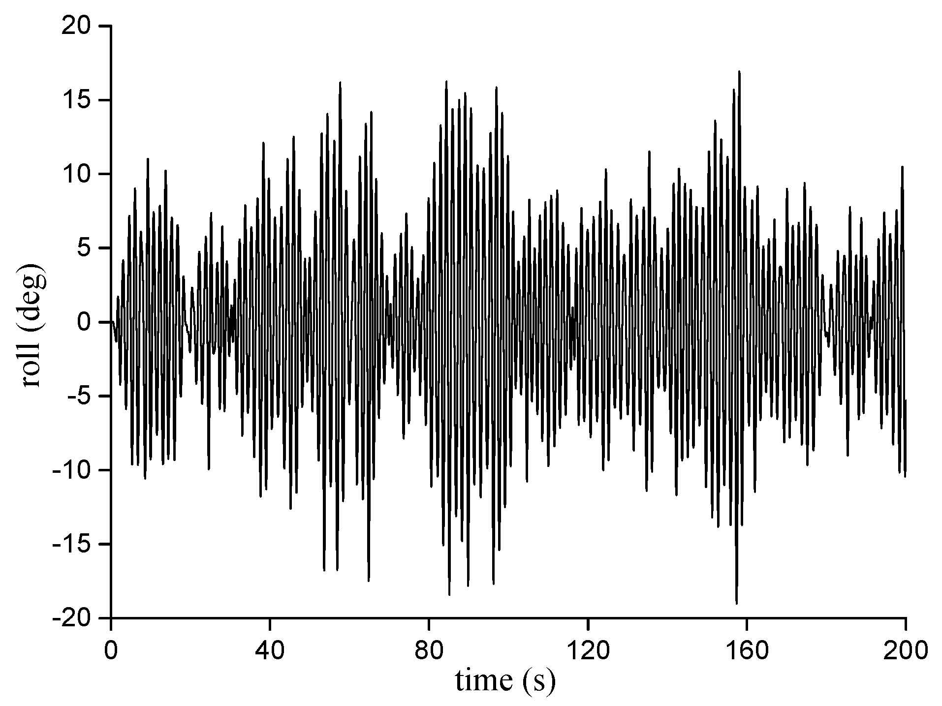
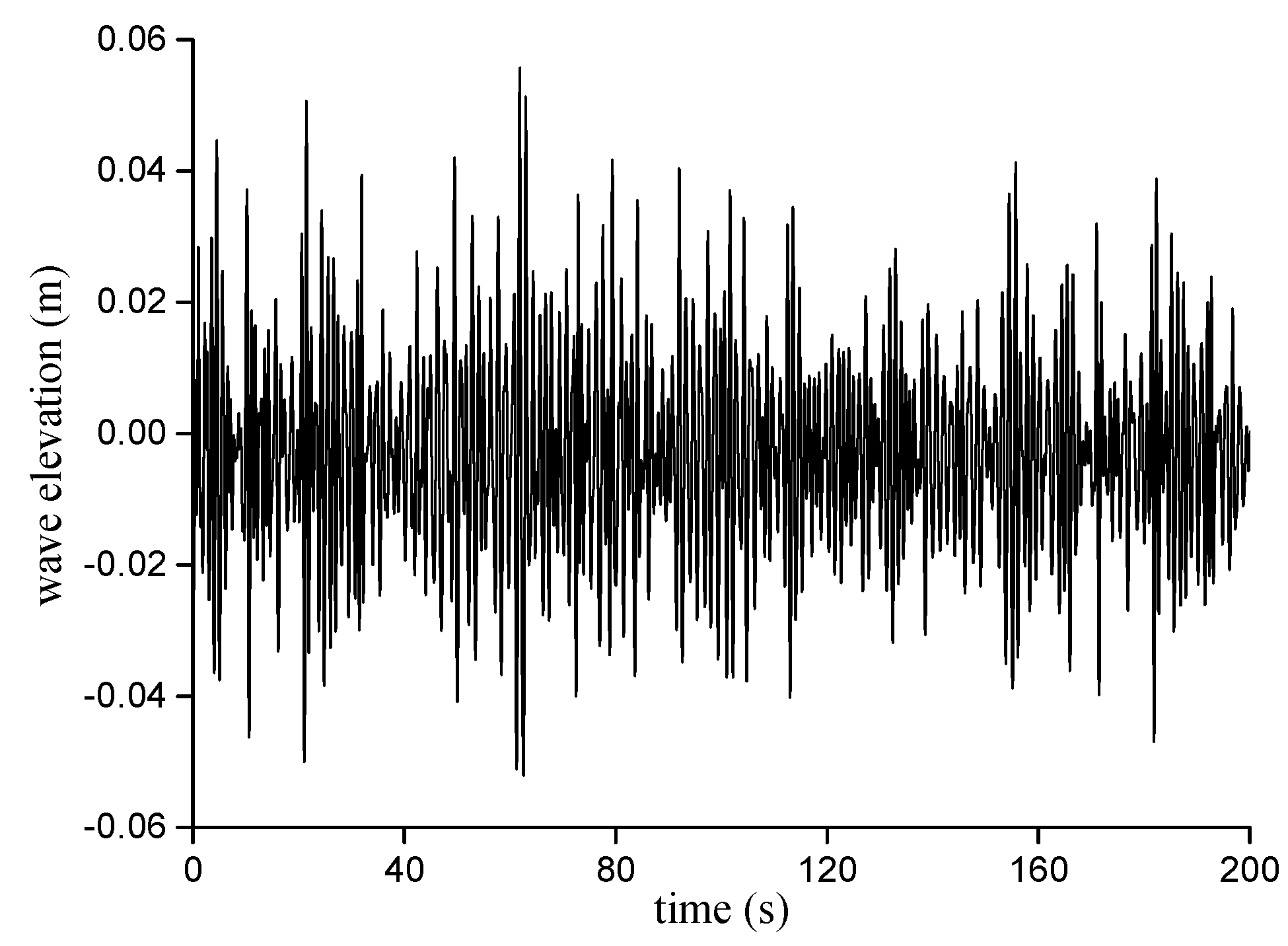
There are four groups of monitoring data in the CFD simulation. One group is the ship roll motion data. Three groups are the wave elevation data at the position 1 m, 3 m, and 5 m away from the ship side in the direction of the incoming wave. Figure 3 shows the ship rolling time-history. Figure 4 shows the wave elevation time-history at the position of 3 m away from the ship’s side. The number of simulation data in each group is 5000. The sampling interval is 0.04 s. The total duration is 200 s. The first 4000 data are selected for model training data. The data for model validation start from the 4500th component.

4. Prediction based on LSTM

4.1. Prediction Solely Using Roll Data

Based on the LSTM model, the roll motion duration data are used as the input feature to directly predict the roll motion with a different advance time. The advance forecast steps n is tested from 5 to 70. The sampling interval is 0.04 s. The advance forecast duration in the model scale is from 0.2 s to 2.8 s, which is converted to 1.4 s to 20 s in full scale.
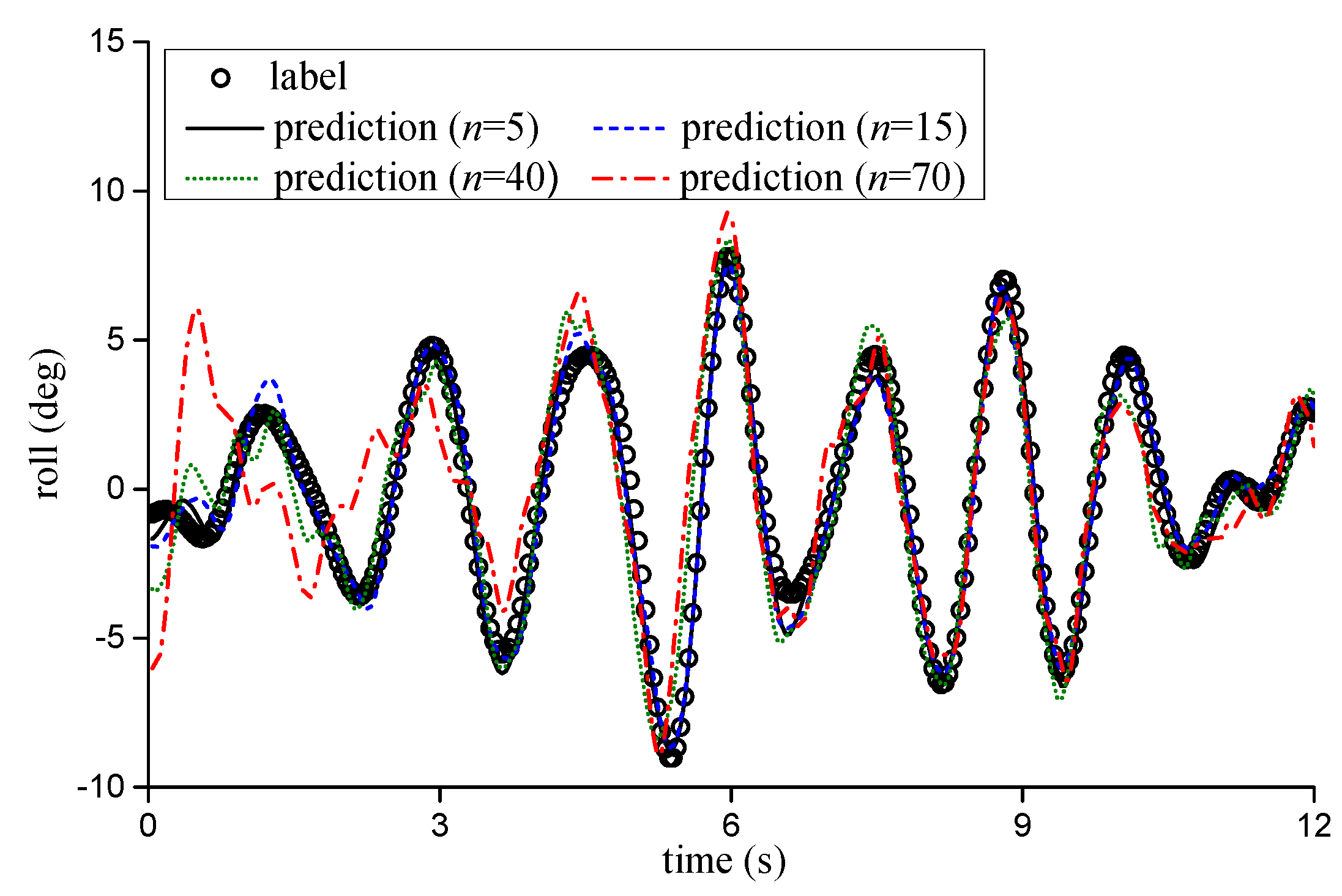
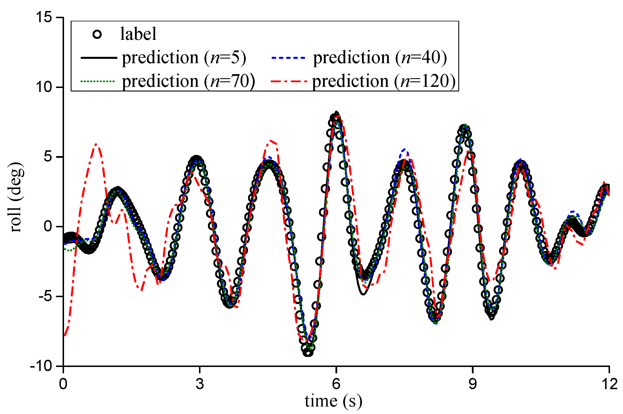
The roll prediction errors solely based on the roll data are shown in Table 3. The comparison between the predicted values of the advance prediction steps n of 5, 15, 40, and 70 and the sample data in the time series are shown in Figure 5. When the number of the advance prediction step is 5, the prediction accuracy is the best. The prediction results are basically matched with the sample values. When the prediction interval step is 70, the accuracy of the prediction results is poor. There is a large deviation between the prediction value and the sample value. This is because the correlation between the time series data weakens the prediction accuracy, which gradually declines with the increase in the advance forecast duration. The results show that the number of effective advance prediction steps solely utilizing the input data of roll cannot exceed 70.

4.2. Prediction Combining with Single-Wave Data

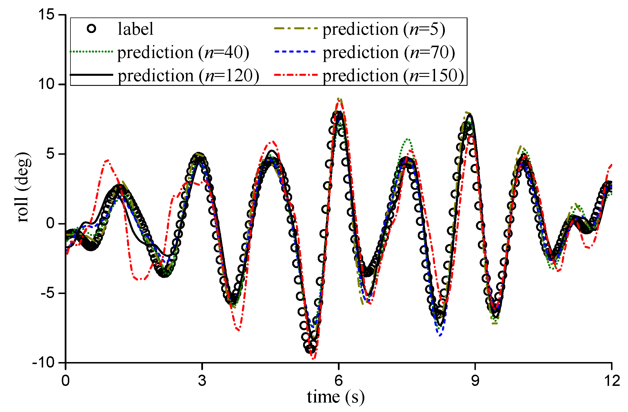
Combined with the ship roll data and the wave elevation data, the roll motion is predicted for a different advance time. The advance prediction steps n based on the wave elevation input at 1 m from the ship’s side are 5, 10, 15, 20, 30, 40, 50, 60 and 70. The number of advance prediction steps based on the wave elevation input at 3 m from the ship’s side increases to 120. The number of advance prediction steps based on the wave elevation input at 5 m from the ship’s side increases to 160. The errors of the prediction results with different input schemes are summarized in Table 4. The results solely based on the ship’s own roll data are also listed in the table. Figure 6, Figure 7 and Figure 8 show the comparison between the time series of roll prediction and the sample data.
Compared with the prediction results solely based on roll input, when the wave elevation data at 1 m from the ship’s side are also taken as the input feature, the overall prediction accuracy is greatly improved. Because the wave is the excitation of the ship rolling, the wave and roll data are related. When roll data and wave elevation data are used as input features for training, the LSTM can mine more effective features for roll prediction. By comparing the prediction results of three wave data inputs, the longer the input wave measurement point is from the ship, the longer will the effective advance prediction time of the ship roll take to gradually increase, although the corresponding prediction accuracy still gradually declines. On the one hand, because of the memory effect of the waves, with the increase in the distance between waves and ships, the time of propagation in space needs to be longer, which can effectively improve the prediction duration. On the other hand, the response relationship between the wave and ship motions will weaken with the increase in distance, resulting in the decline of the prediction accuracy. Combined with the wave data at 5 m from the ship, the number of advance steps for ship roll prediction can reach 120.

4.3. Prediction Combining with Multiple-Wave Data

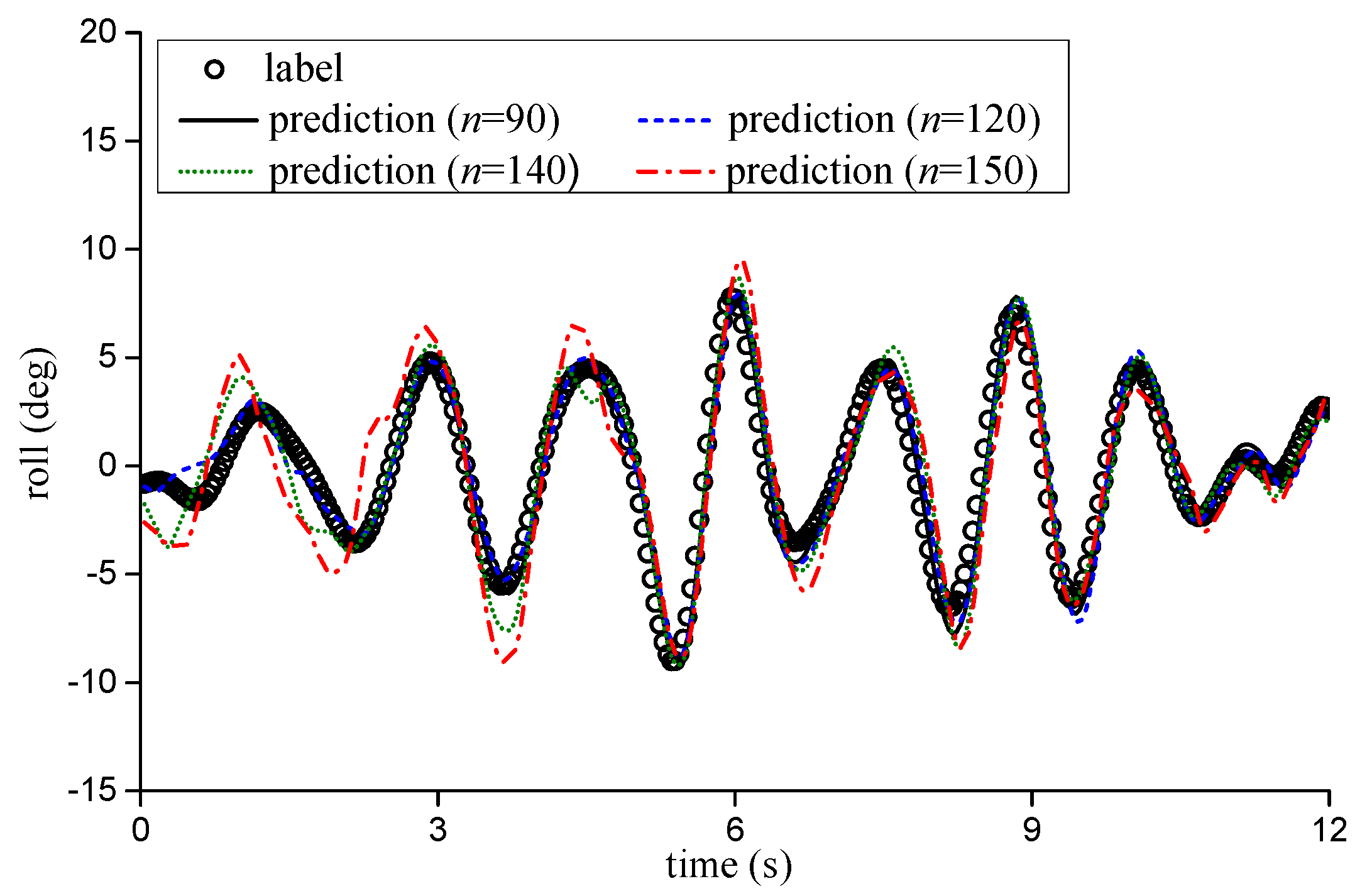
In order to explore the relationship between waves and ship motions, the effect of multiple-wave elevation data as input characteristics on the roll motion prediction is studied. Based on three sets of wave elevation data at 1 m, 3 m, and 5 m from the ship’s side, three different wave elevation data schemes and roll data are combined as input features for roll motion prediction. The three wave elevation input forms are based on the wave elevation data at 1 m and 3 m, at 3 m, and 5 m and at 1 m, 3 m, and 5 m. The comparison between the time series of the ship roll predicted based on different input schemes and the sample value is shown in Figure 9, Figure 10 and Figure 11. The roll prediction error is summarized in Table 5.
The prediction results based on multiple-wave data have better stability than those based on single-wave data. When the input scheme combines the wave elevation data of 1 m and 3 m from the ship, compared with the prediction scheme with the input wave height of 1 m from the ship, the prediction accuracy decreases with a small advance prediction step (n ≤ 30), but the prediction accuracy increases significantly in case of a large advance prediction step (n ≥ 40). Compared with the prediction scheme with the input wave height of 3 m from the ship, the prediction accuracy based on the two sets of wave input has greatly improved even if the number of advance prediction step is small. With the increase in the number of prediction steps, the prediction accuracy is equivalent to both. When the input scheme is combined with the wave data at 1 m, 3 m, and 5 m from the ship, the stability of the prediction results is improved to a certain extent compared with that based on the two sets of wave input, especially when the advance prediction step is smaller. The prediction accuracy is improved significantly. The number of advance step for the ship roll prediction can reach 150 by combining the three sets of the wave input scheme. Because the wave elevations at different locations have different optimal advance prediction durations, the LSTM neural network could extract the optimal weights of the multiple wave elevations. When the different advance prediction durations are used, the stability of the prediction could be improved as a whole.

5. Conclusions

Based on the LSTM neural network, this paper studies the very short-term prediction of the ship roll motion considering the wave elevation input. The influence of the wave data input on the prediction accuracy and the advance prediction duration is analyzed. Using the wave elevation and ship motion data, the feasibility of considering the wave elevation input to predict the ship roll motion is verified. The following conclusions are obtained.
(1)
Compared with the prediction results solely based on the roll data input, the roll motion prediction considering the wave elevation input greatly improves both the prediction accuracy and the advance prediction duration;
(2)
For single-wave data input, the LSTM model can mine the mapping relationship between the advance prediction duration and the distance of the wave height measurement points. The effective advance prediction time increases with the increase in the distance from the wave gauge to the ship;
(3)
Compared with the prediction results of the single-wave data input, the prediction of the multiple-wave data input has better stability for different advance times. As the amount of data increases, the overall advance prediction duration of the LSTM model improves, and the model also has better robustness for larger advance prediction durations.

Author Contributions

Conceptualization, X.T.; Y.S.; methodology, X.T.; software, X.T.; validation, X.T.; Y.S.; formal analysis, X.T.; investigation, X.T.; resources, X.T.; data curation, Y.S.; writing—original draft preparation, X.T.; writing—review and editing, X.T.; visualization, X.T.; supervision, Y.S.; project administration, X.T.; funding acquisition, Y.S. All authors have read and agreed to the published version of the manuscript.

Funding

This research received no external funding.

Institutional Review Board Statement

Not applicable.

Informed Consent Statement

Not applicable.

Data Availability Statement

Data is unavailable due to privacy.

Conflicts of Interest

The authors declare no conflict of interest.

References

  1. Triantafyllou, M.; Bodson, M.; Athans, M. Real time estimation of motions of a destroyer using Kalman filtering techniques. IEEE J. Ocean. Eng. 1983, 8, 9–20. [Google Scholar] [CrossRef]
  2. Zhao, X.; Xu, R.; Kwan, C. Ship-motion prediction: Algorithms and simulation results. In Proceedings of the IEEE International Conference on Acoustics, Montreal, QC, Canada, 17–21 May 2004; IEEE: New York, NY, USA; Volume 5, pp. 125–128. [Google Scholar]
  3. Li, G.; Kawan, B.; Wang, H.; Zhang, H. Neural-network-based modelling and analysis for time series prediction of ship motion. Ship Technol. Res. 2017, 64, 30–39. [Google Scholar] [CrossRef]
  4. Suhermi, N.; Prastyo, D.D.; Ali, B. Roll motion prediction using a hybrid deep learning and ARIMA model. Procedia Comput. Sci. 2018, 144, 251–258. [Google Scholar] [CrossRef]
  5. Duan, W.Y.; Huang, L.; Yang, H.; Wang, R. IRF-AR model for short-term prediction of ship motion. In Proceedings of the Twenty-Fifth International Offshore and Polar Engineering Conference, Hawaii, HI, USA, 21–26 June 2015. ISOPE-I-15-584. [Google Scholar]
  6. Yin, J.C.; Perakis, A.N.; Wang, N. A real-time ship roll motion prediction using wavelet transform and variable RBF network. Ocean. Eng. 2018, 160, 10–19. [Google Scholar] [CrossRef]
  7. Li, M.; Geng, J.; Hong, W. Periodogram estimation based on LSSVR-CCPSO compensation for forecasting ship motion. Nonlinear Dyn. 2019, 97, 2579–2594. [Google Scholar] [CrossRef]
  8. Duan, W.; Huang, L.; Han, Y. A hybrid AR-EMD-SVR model for the short-term prediction of nonlinear and non-stationary ship motion. J. Zhejiang Univ. Sci. A 2015, 16, 562–576. [Google Scholar] [CrossRef]
  9. Shen, Y. On the Neural Network Theory and its Application in Ship Motion Prediction. Ph.D. Thesis, Harbin Engineering University, Harbin, China, 2005. [Google Scholar]
  10. Hochreiter, S.; Schmidhuber, J. Long short-term memory. Neural Comput. 1997, 9, 1735–1780. [Google Scholar] [CrossRef] [PubMed]
  11. Wang, G.; Han, B.; Sun, W. Short-term prediction of ship motion based on LSTM. Ship Sci. Technol. 2017, 39, 69–72. [Google Scholar]
  12. D’Agostino, D.; Serani, A.; Stern, F.; Diez, M. Recurrent-type neural networks for real-time short-term prediction of ship motions in high sea state. arXiv 2021, arXiv:2105.1310. [Google Scholar] [CrossRef]
  13. Zhang, W.; Wu, P.; Peng, Y.; Liu, D. Roll motion prediction of unmanned surface vehicle based on coupled CNN and LSTM. Future Internet 2019, 11, 243. [Google Scholar] [CrossRef]
  14. Zhang, B.; Peng, X.; Gao, J. Ship motion attitude prediction based on ELM-EMD-LSTM integrated model. J. Ship Mech. 2020, 24, 1413–1421. [Google Scholar]
  15. Peng, X.; Zhang, B.; Zhou, H. An improved particle swarm optimization algorithm applied to long short-term memory neural network for ship motion attitude prediction. Trans. Inst. Meas. Control 2019, 41, 4462–4471. [Google Scholar] [CrossRef]
  16. Geng, X.; Li, Y.; Sun, Q. A Novel Short-Term Ship Motion Prediction Algorithm Based on EMD and Adaptive PSO–LSTM with the Sliding Window Approach. J. Mar. Sci. Eng. 2023, 11, 466. [Google Scholar] [CrossRef]
  17. Zhang, T.; Zheng, X.; Liu, M. Multiscale attention-based LSTM for ship motion prediction. Ocean. Eng. 2021, 230, 109066. [Google Scholar] [CrossRef]
  18. Sun, Q.; Tang, Z.; Gao, J.; Zhang, G. Short-term ship motion attitude prediction based on LSTM and GPR. Appl. Ocean. Res. 2022, 118, 102927. [Google Scholar] [CrossRef]
  19. Wang, Y.; Wang, H.; Zou, D.; Fu, H. Ship roll prediction algorithm based on Bi-LSTM-TPA combined model. J. Mar. Sci. Eng. 2021, 9, 387. [Google Scholar] [CrossRef]
  20. Wang, Y.; Wang, H.; Zhou, B.; Fu, H. Multi-dimensional prediction method based on Bi-LSTMC for ship roll. Ocean. Eng. 2021, 242, 110106. [Google Scholar] [CrossRef]
  21. Tang, G.; Lei, J.; Shao, C.; Hu, X.; Cao, W.; Men, S. Short-term prediction in vessel heave motion based on improved LSTM model. IEEE Access 2021, 9, 58067–58078. [Google Scholar] [CrossRef]
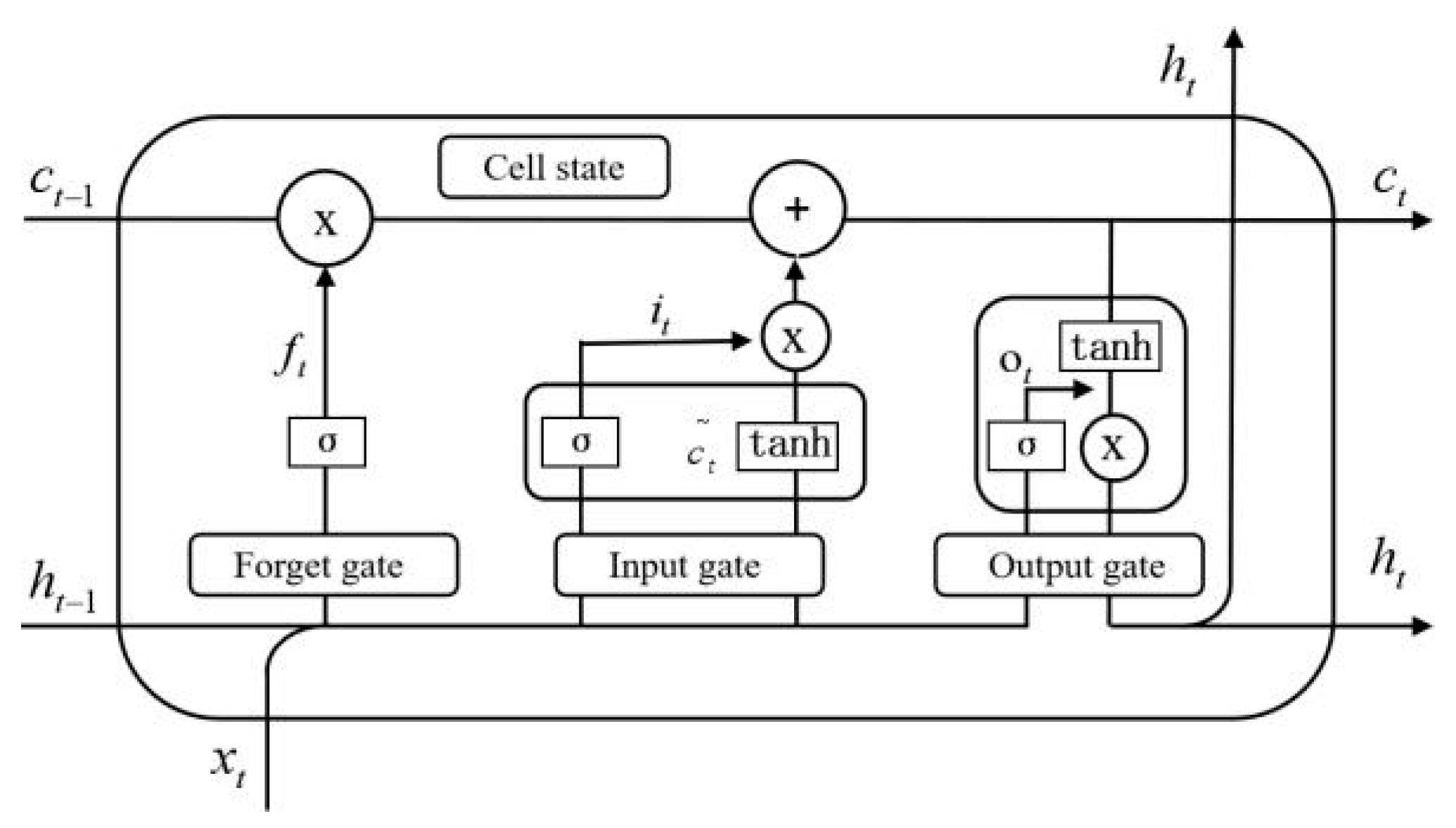
Figure 1. LSTM structure.
Applsci 13 05298 g001
Figure 2. LSTM input and output data mapping diagram.
Applsci 13 05298 g002
Figure 3. Time series of roll motion obtained by CFD simulation.
Applsci 13 05298 g003
Figure 4. Time series of wave elevation obtained by CFD simulation (wave probe 3 m from ship).
Applsci 13 05298 g004
Figure 5. Time series of roll prediction solely using data of roll input.
Applsci 13 05298 g005
Figure 6. Time series of roll prediction combining wave data 1 m from ship.
Applsci 13 05298 g006
Figure 7. Time series of roll prediction combining wave data 3 m from ship.
Applsci 13 05298 g007
Figure 8. Time series of roll prediction combining wave data 5 m from ship.
Applsci 13 05298 g008
Figure 9. Time series of roll prediction combining wave data 1 m and 3 m from ship.
Applsci 13 05298 g009
Figure 10. Time series of roll prediction combining wave data 3 m and 5 m from ship.
Applsci 13 05298 g010
Figure 11. Time series of roll prediction combining wave data 1 m, 3 m and 5 m from ship.
Applsci 13 05298 g011
Table 1. Summarization of machine learning models for ship motion prediction.
ModelInputReference
KFswayTriantafyllou and Bodson (1982) [1]
MCA6-DoF motionZhao et al. (2004) [2]
NARXstate attributeLi et al. (2017) [3]
DNN-ARrollSuhermi et al. (2018) [4]
IRF-ARheave, pitchDuan et al. (2015) [5]
DWT-RBFrollYin et al. (2018) [6]
SVR-PSOrollLi and Hong (2019) [7]
AR-EMD-SVRheave, pitchDuan et al. (2015) [8]
RNN6-DoF motionShen (2005) [9]
LSTMroll, pitchWang et al. (2017) [11]
GRUstate attributeD’Agostino et al. (2021) [12]
CNN-LSTMrollZhang et al. (2019) [13]
EMD-LSTMmotionZhang et al. (2020) [14]
PSO-EMD-LSTMroll, pitch, heavePeng et al. (2019) [15]
EMD-PSO-LSTMroll, pitchGeng et al. (2023) [16]
AM-LSTM6-DoF motionZhang et al. (2021) [17]
LSTM-GPRroll, pitchSun et al. (2022) [18]
BLSTM-TPArollWang et al. (2021) [19]
MISO-BLSTM-TPArollWang et al. (2021) [20]
Table 2. Ship information.
ParameterFull ScaleModel Scale (1/51)
Water line (m)142.182.79
Breadth (m)19.060.37
Draft (m)6.150.12
Displacement (m3)84240.0635
Table 3. Roll prediction solely using data of roll input.
Advance Prediction StepModel ScaleFull ScalePrediction Error (deg)
RMSEMAE
50.2 s1.4 s0.431.41
100.4 s2.9 s0.541.53
150.6 s4.3 s0.571.58
200.8 s5.7 s0.813.12
301.2 s8.6 s1.313.48
401.6 s11.4 s1.364.29
502.0 s14.3 s1.514.35
602.4 s17.1 s1.574.48
702.8 s20.0 s2.227.60
Table 4. Roll prediction combining with single-wave data (unit: deg).
Advance Prediction StepNo Wave Data1 m from Ship3 m from Ship5 m from Ship
RMSEMAERMSEMAERMSEMAERMSEMAE
50.431.410.280.980.441.390.792.48
100.541.530.250.980.511.580.842.84
150.571.580.260.900.501.580.862.94
200.813.120.270.770.561.641.043.10
301.313.480.351.010.531.920.872.55
401.364.290.501.290.531.630.902.20
501.514.351.023.200.551.800.852.22
601.574.481.243.690.561.670.942.71
702.227.601.853.900.571.720.912.25
800.661.910.962.59
900.942.430.922.47
1001.133.270.982.70
1101.695.671.002.47
1202.197.021.062.24
1301.233.13
1401.403.58
1501.945.03
1602.587.30
Table 5. Roll prediction combining with multiple-wave data (unit: deg).
Advance Prediction Step1 m and 3 m
from Ship
3 m and 5 m
from Ship
1 m, 3 m and 5 m
from Ship
RMSEMAERMSEMAERMSEMAE
50.290.970.421.170.321.12
100.290.880.481.450.401.38
150.321.150.491.650.301.01
200.371.280.511.550.320.92
300.381.180.541.370.391.20
400.451.160.601.520.471.46
500.561.570.601.600.561.59
600.541.690.661.890.601.66
700.601.650.631.860.611.82
800.712.320.681.930.621.60
900.962.940.692.040.651.85
1001.273.730.792.060.782.05
1101.654.290.932.510.902.32
1202.045.710.932.850.912.29
1301.112.811.102.36
1401.302.971.232.54
1501.934.551.924.27
1602.376.082.305.79
Disclaimer/Publisher’s Note: The statements, opinions and data contained in all publications are solely those of the individual author(s) and contributor(s) and not of MDPI and/or the editor(s). MDPI and/or the editor(s) disclaim responsibility for any injury to people or property resulting from any ideas, methods, instructions or products referred to in the content.