Article

Electronic Atlas of Climatic Changes in the Western Russian Arctic in 1950–2021 as Geoinformatic Support of Railway Development

by
Alexei D. Gvishiani
1,2,
Igor N. Rozenberg
3,
Anatoly A. Soloviev
1,2,
Andrey G. Kostianoy
1,4,5,
Sofia A. Gvozdik
1,6,*,
Ilya V. Serykh
1,4,
Roman I. Krasnoperov
1,
Nikolay V. Sazonov
7,
Irina A. Dubchak
3,
Anton B. Popov
1,
Evgenia A. Kostianaia
1,4 and
Georgy A. Gvozdik
1,6
1
Geophysical Center of the Russian Academy of Sciences, 119296 Moscow, Russia
2
Schmidt Institute of Physics of the Earth of the Russian Academy of Sciences, 123242 Moscow, Russia
3
Russian University of Transport, 127994 Moscow, Russia
4
Shirshov Institute of Oceanology of the Russian Academy of Sciences, 117997 Moscow, Russia
5
Sergei Witte Moscow University, 115432 Moscow, Russia
6
Geological Faculty, Lomonosov Moscow State University, 119234 Moscow, Russia
7
Research and Design Institute of Informatization, Automation and Communications in Railway Transport, 109029 Moscow, Russia
*
Author to whom correspondence should be addressed.
Appl. Sci. 2023, 13(9), 5278; https://doi.org/10.3390/app13095278
Submission received: 21 February 2023 / Revised: 8 April 2023 / Accepted: 18 April 2023 / Published: 23 April 2023
(This article belongs to the Collection Geoinformatics and Data Mining in Earth Sciences)

Abstract

:
The Arctic zone of the Russian Federation is one of the most intensively developing regions of the country. Amongst the major domains of economic and industrial growth and improvement is transport infrastructure and particularly the railway network. This area is being exposed to negative factors of rapid climate change that can significantly affect and compromise this activity. Thus, it is vital to take them into account during design, construction, and operation of the railway infrastructure facilities. This work details the production of a digital atlas comprising the 1950–2021 dynamics of the main hydrometeorological parameters: air and soil temperature, precipitation, wind speed, air and soil humidity, and snow cover thickness. The maps are based on climatic data derived from the MERRA-2 (Modern-Era Retrospective Analysis for Research and Applications, version 2) reanalysis. In total there are 459, which are arranged into 7 chapters. The atlas geographically covers the western part of the Russian Arctic encompassing the regions of quite intensive transport development, which includes the construction of the Northern Latitudinal Railway. Original algorithms of geospatial data processing and their further representation as well as the maps compiled in GIS environment are discussed. Comprehensive analysis of climatic changes in the region of the Russian Arctic including detailed quantitative evaluation over 40 years is given. In the Discussion, we focus on those changes of the regional climate which, from our point of view, are the most significant for consideration by railway operators. The obtained results contribute to framing the theoretical basis of design, development, and sustainable operation of the railway infrastructure in the Arctic and facilitate the decision-making process. This is the first experience of building a specialized climatic cartographic product for the needs of the Russian railways, and to our knowledge the first atlas such as that in the world. In the future, the amassed experience may be transferred to other regions of the Russian Federation as well as similar regions in Canada, Sweden and Highland China that are also subject to significant climate change.

1. Introduction

The Arctic zone of the Russian Federation (AZRF) is exposed to the factors of climate change that drastically affect numerous natural (seas, lakes, rivers, forests, tundra, landscapes, soils, biodiversity, etc.) and socio-economic (population, demography, human resources, employment, health of people, industry, oil and gas production, mining of coal, metal ores, diamonds, fishery, agriculture, forestry, water management, energy production and transportation, aerial, road, railway and water transport, etc.) systems of this territory [1]. On 10 October 2022, the Russian Federal Service for Hydrometeorology and Environmental Monitoring (Roshydromet) issued the “Third Assessment Report on Climate Change and its Consequences in the Territory of the Russian Federation” [1]. The major conclusion in this report states that the entire territory of the country is warming at an average rate of 0.51 °C per decade while the AZRF is warming at an average rate of 0.71 °C per decade. According to current forecasts, the area occupied by near-surface permafrost in the territory of Russia will decrease by the middle of the 21st century according to the SSP2-4.5 scenario by 22 ± 7% and for the SSP5-8.5 scenario by 28 ± 10% as compared to the period 1995–2014. By the end of the 21st century, this reduction is expected to be at the level of 40 ± 15% and 72 ± 20%, respectively [1,2].
The subarctic zone of Russia hosts vast oil and gas, sea, railway, and pipeline transport infrastructure worth hundreds of billions of dollars. This region being covered with permafrost is also vulnerable to climate change because the thawing of frozen layers due to significant ice content may cause an average soil settlement of 10–20 cm per year [2], which is critical for pile structures and the entire transport infrastructure in general [3,4]. Serykh et al. [5] showed that in 1999–2020, the Republic of Karelia, Murmansk and Arkhangelsk Oblasts (Regions) experienced significant climate warming at a rate from +0.9 °C to +1.5 °C as compared to previous years (1977–1998). A sharp increase in air temperature at a rate from +0.4 °C to +1.0 °C per decade resulted in the displacement of the +2 °C isotherm for 550 km northwards up to the White Sea southern part and induced the total disappearance of average negative temperatures in the Republic of Karelia, Murmansk and Arkhangelsk Oblasts.
The railway infrastructure in the subarctic territories of Russia is naturally operated in extremely difficult geological and climatic conditions, being exposed to the continuous negative impact of various external factors, leading to deformation of railway tracks and damage of artificial structures [1,3]. Thawing of permafrost soils and significant increase in average temperature cause further changes in the water balance of numerous rivers and lakes in this region. These processes intensify coastal abrasion, erosion, mudflows, floods, landslides, ground creep, rockfalls, rockslides, karst sinkholes, snow avalanches, etc. [1,3,5,6].
Isolated permafrost zones may still be found on the Kola Peninsula [7]. Russian railway facilities in this region are particularly vulnerable to the negative factors of regional climate change, considering their intense development. It is planned that the Murmansk section of the Oktyabrskaya Railway will increase transportation from 28 to 44 million tons per year by 2023, and by 2035 it should grow up to 100 million tons. At the same time, some railway sections are still single-track, which limits their carrying capacity [8].
Extensive railway infrastructure is located in the Northwestern and Ural Federal Districts of Russia. The Northwestern Federal District (NFD) covers 9.8% of the country’s territory; 9.5% of the Russian population lives here [9]. In this district, the railway infrastructure runs through the territory of the Republic of Karelia, Murmansk and Arkhangelsk Oblasts, the Komi Republic, and the Nenets Autonomous Okrug (District).
Let us consider the main aspects of the NFD economic development. The turnover of organizations of all types of economic activity in the first quarter of 2022 amounted to 175.7 billion dollars, or 176.2% of the level of the first quarter of 2021. Sales per capita were equal to 1110 dollars (the average parameter in Russia was 1002 dollars). The volume of investment in fixed capital in the economic and social development of the district in the first quarter of 2022 amounted to 5.4 billion dollars, or 103.4% of the level of the corresponding period in 2021. The consolidated budget of the NFD regions had a surplus of 2.3 billion dollars in the first quarter of 2022. Thus, revenues amounted to 7.5 billion dollars, and expenditures were 5.3 billion dollars.
The Ural Federal District (UFD) covers 10.6% of the territory of Russia; 8.4% of the Russian population lives here [10]. In this district, the railway infrastructure runs through the territory of Khanty-Mansi and Yamalo-Nenets Autonomous Okrugs. The turnover of organizations of all types of economic activity in the first quarter of 2022 was 147.3% compared with the same period in 2021, or 134.3 billion dollars. Sales per capita were equal to 949 dollars. The volume of investment in fixed assets of the district economy and social sphere in first quarter of 2022 amounted to 11.1 billion dollars, or 118.7% of the level of the corresponding period in 2021. The consolidated budget of the UFD regions in the first quarter of 2022 had a surplus of 1.6 billion dollars. Thus, revenues amounted to 6.6 billion dollars, and expenditures were 5.0 billion dollars.
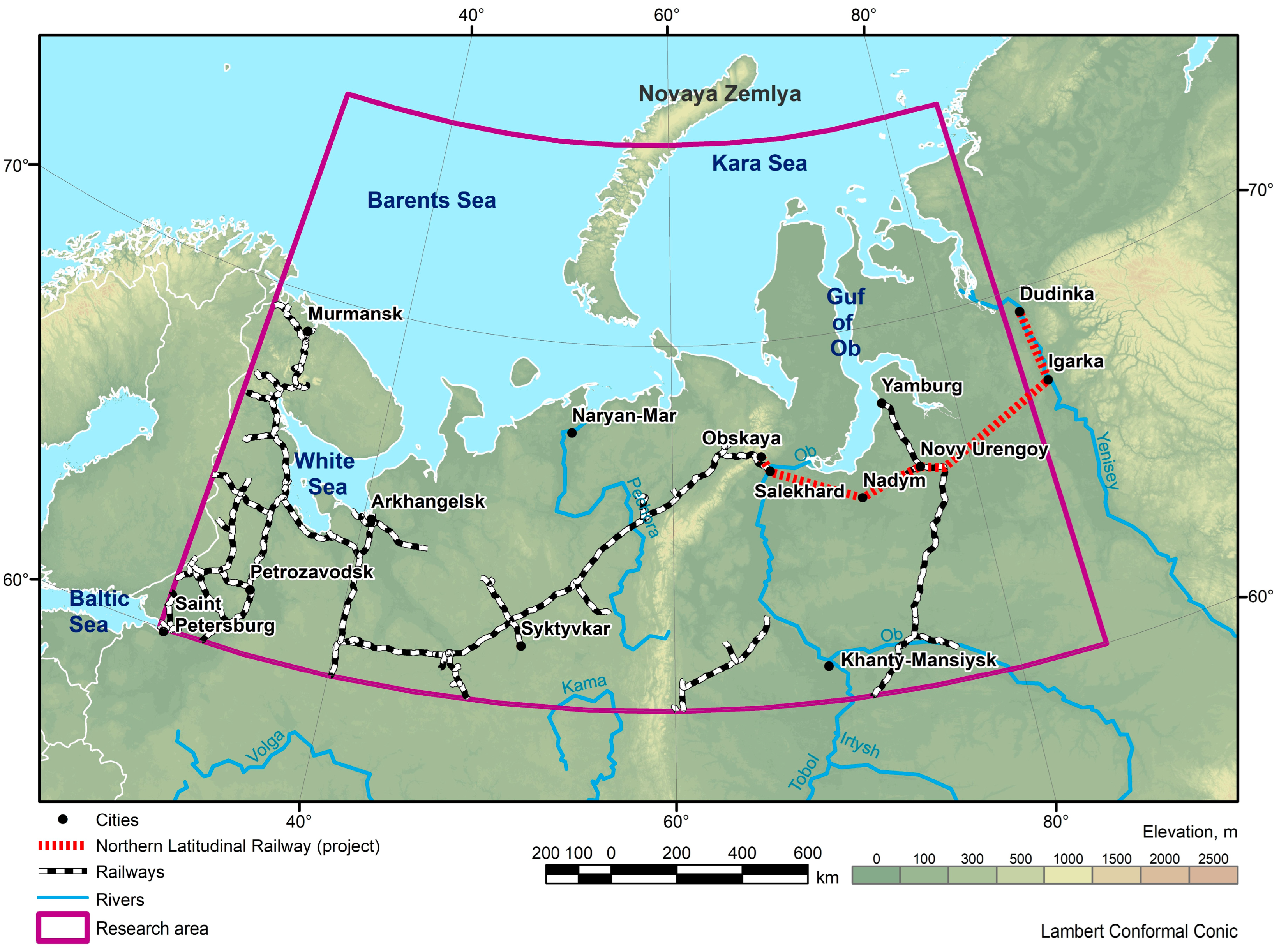
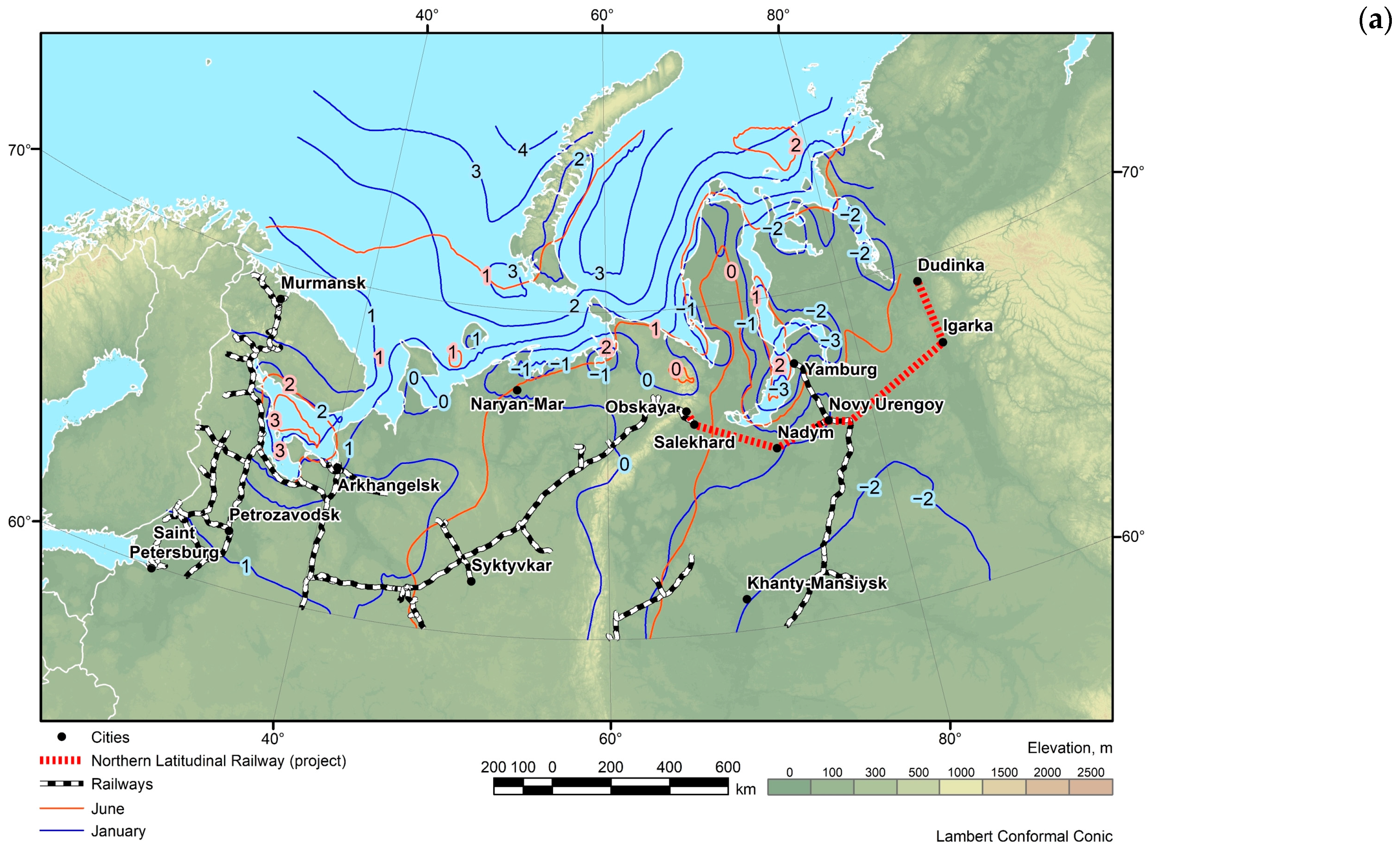
The abovementioned economic parameters indicate the accelerated development of these territories. In this regard, an extensive network of railways and smooth operation of their infrastructure has become increasingly important. For example, the current Northern Latitudinal Railway (NLR) project is critically important for the development of the Yamalo-Nenets Autonomous Okrug (YaNAO). NLR is a 686 km long railway that is being built along the line Obskaya–Salekhard–Nadym–Novy Urengoy–Korotchaevo in Figure 1. This projected railway will connect the western and eastern parts of the YaNAO [11]. It will sustain comprehensive economic growth of the northern territories, provide infrastructure for the development of gas-condensate and oil fields, and ensure the transportation of extracted natural resources. The implementation of the NLR project will form the infrastructure that will contribute to the expansion of the tanker fleet and efficient development of the Arctic resources. NLR will facilitate the direct access to the Northern Sea Route through the port of Sabetta in the Yamal Peninsula. This project will also produce jobs for the Russian railways and servicing industries [12]. After the project completion, the estimated traffic volume will be about 24 million tons, primarily as gas condensate and oil cargo.
As the part of the NLR implementation, construction of the Bovanenkovo–Sabetta railway section or the so-called NLR-2 project is planned. In the future, up to 2030, it is planned to extend the railway from Korotchaevo eastwards to the Yuzhno-Russkoye oil and gas field (122 km) and from this point to the port of Igarka via Ermakovo (482 km). As a farther perspective, there are plans to build the Igarka–Dudinka railway eastwards with a subsequent connection to the Norilsk railway in Figure 1. This project is called the “eastern arm” of the NLR.
In this regard, research on climate change in the Republic of Karelia, Murmansk and Arkhangelsk Oblasts, Komi Republic, Yamalo-Nenets and Khanty-Mansi Autonomous Okrugs using modern geoinformatic tools is extremely important for the Russian railways’ operation.
The core goal of the present work is the production of the digital atlas for tracking climatic variations of basic hydrometeorological parameters in the western part of the Russian Arctic (60–75° N, 30–85° E) over 1950–2021 based on the MERRA-2 atmospheric reanalysis dataset. The article describes the main hydrometeorological parameters forming the atlas: surface air temperature, total precipitation, wind speed at the Earth’s surface, soil temperature, soil moisture content, air humidity, and snow cover thickness. The methodology of the map compilations is described in detail. For each of the parameters, we present its brief characteristics, methods of measurement, and provide examples of the different map types. Comprehensive assessment of regional changes in climatic parameters was previously performed for the Russian Arctic, e.g., for the Barents Sea [13]. The most significant results of studying the inter-annual variability of certain climatic parameters directly affecting the smooth railway operation are thoroughly discussed. In conclusion, we agree in favor of atlas expansion that will ensure the theoretical basis for sustainable development and operation of the Russian railways in the Arctic zone.
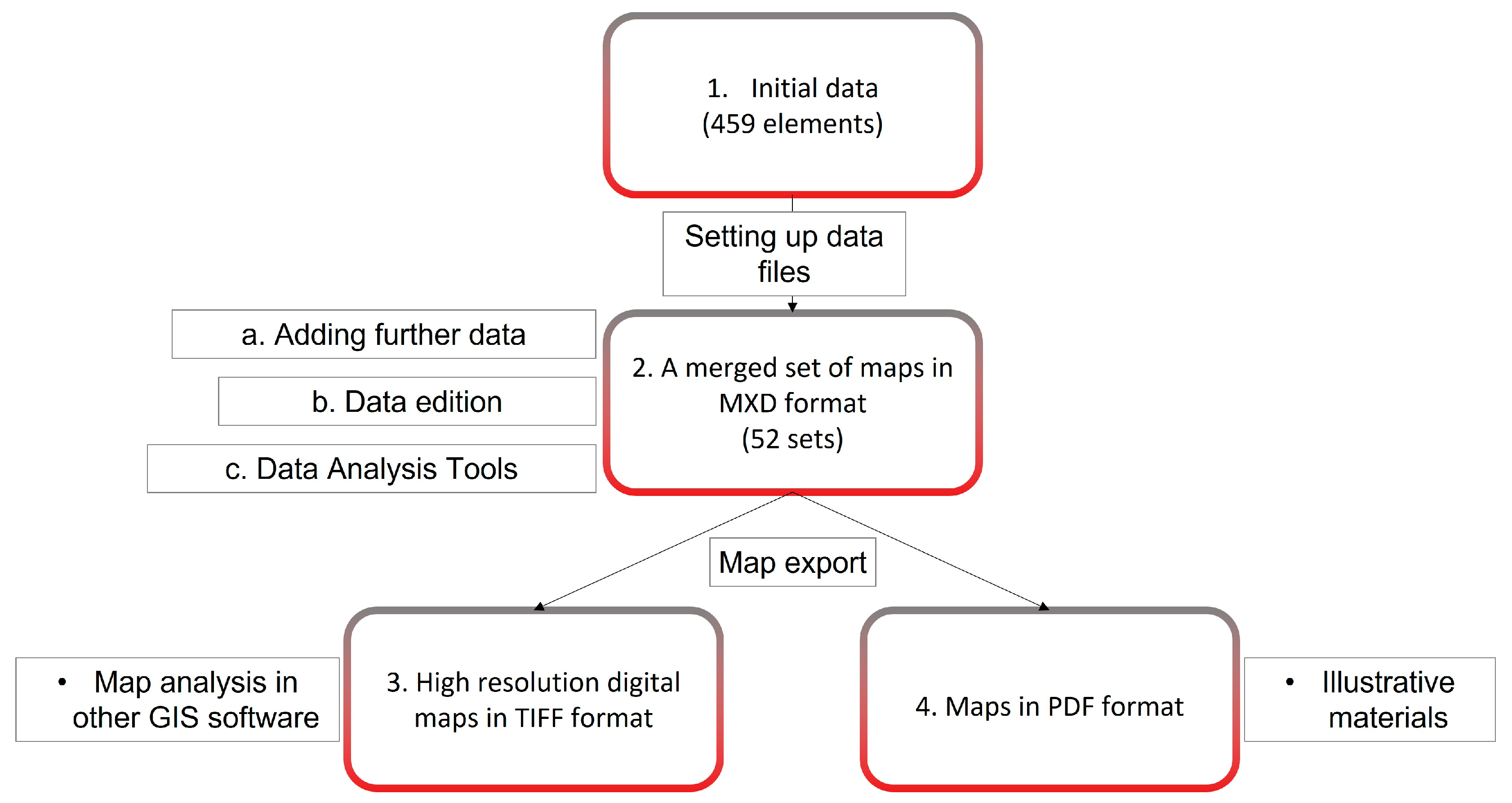
Thus, the novelty of the research is in building of a specialized digital climate atlas for the needs of the Russian Railways in the western part of the Russian Arctic and in the subsequent analysis of change of basic meteorological parameters which may impact operability of the existing railway network and its development in future. Building of the atlas required development of original algorithms of geospatial data processing and their further representation, as well as the maps compiled in a GIS environment based on the MERRA-2 atmospheric reanalysis for the past 40 years. Comprehensive analysis of climatic changes included 7 hydrometeorological parameters presented in different characteristics in 459 maps.

2. Data and Methods

2.1. Studied Area

The studied area includes the western part of the Russian Arctic within the geographical boundaries 60–75° N, 30–85° E in Figure 1. It includes the Republic of Karelia, Murmansk and Arkhangelsk Oblasts (Regions), Komi Republic, Yamalo-Nenets and Khanty-Mansi Autonomous Okrugs (Districts). Within this area there are railway sections between St. Petersburg and Murmansk and Arkhangelsk, railways to Salekhard and Yamburg, the 700km section of the constructed NLR from the Obskaya station (Labytnangi) to Korotchaevo (Novy Urengoy), and the next section to Igarka and further to Dudinka in Figure 1.

2.2. Initial Data for Climatic Atlas Maps

For a production of maps of hydrometeorological parameters (surface air temperature, total precipitation, wind speed at the Earth’s surface, soil temperature, soil moisture content, air humidity, and snow cover thickness) presented in the atlas, the authors used the MERRA-2 reanalysis data for the period 1980–2021.
MERRA-2 dataset (Modern-Era Retrospective Analysis for Research and Applications, version 2) [14] represents the results of reprocessing of a massive catalog of information on climatic parameters, such as air temperature and humidity, atmospheric pressure, wind speed, precipitation, etc. Generally, the database is a set of global daily data on the state of the atmosphere and the Earth’s surface, collected over several decades. This mission was implemented at the Global Modeling and Assimilation Office (GMAO) under the direction of the U.S. National Aeronautics and Space Administration (NASA).
MERRA was originally created for integration of satellite measurements into a unified climate catalog to facilitate the description of the global hydrological cycle from the Earth’s atmosphere to the surface of the planet. This mission was launched in 1979, but by 2016 it was closed due to certain disadvantages: measurement system errors (e.g., non-physical measurement jumps when the observing system changes), imbalances in some atmospheric and terrestrial hydrological parameters, degraded representation of the upper stratosphere, and system limitations that prevented inclusion of new satellite data sources [14].
The main goal of reprocessing and refining the MERRA mission was to provide continuous near-real-time climate analysis (data are published with delays of a couple of weeks). Accordingly, MERRA-2 was designed as a reanalysis that uses the latest developments in data measurement and processing to address the known limitations and disadvantages of MERRA. The reanalysis provides long-term monitoring and comprehensive analysis of Earth conditions by means of system integration of atmospheric, ocean, land, and physical and chemical information. Other updates include information on ozone monitoring and the use of precipitation observations. On the technical side, the MERRA-2 observing system has been equipped with additional instruments that register the following parameters [15]:
  • Atmospheric motion vectors from AVHRR (Advanced Very High Resolution Radiometer);
  • Surface wind speed from SSMIS (Special Sensor Microwave Imager/Sounder);
  • Temperature profiles and ozone characteristics from EOS (Earth Observing System) Aura MLS (Microwave Limb Sounder);
  • Total amount of ozone in the column from EOS (Earth Observing System) Aura OMI (Ozone Monitoring Instrument);
  • Deviation angle from GPSRO (Global Positioning System Radio Occultation);
  • Microwave sounding from ATMS (Advanced Technology Microwave Sounder);
  • Hyper spectral infrared radiation from IASI (Infrared Atmospheric Sounding Interferometer) on MetOp-A and MetOp-B (Meteorological Operational Satellites) and from CrIS (Cross-Track Infrared Sounder) on SNPP (Suomi National Polar-Orbiting Partnership);
  • Geostationary radiation from MSG (Meteosat Second Generation) SEVIRI (Spinning Enhanced Visible Infrared Imager).
The rest of the observation system remained unchanged as in the original MERRA mission except for improvements of the sensors for measuring surface wind speed and ozone content. These sensors were changed to more advanced models during the mission development.
Today, MERRA-2 is known as one of the most accurate global representations of climatic data for land and ocean [14]. This results from the extensive volume of output data available for processing along with high spatial resolution, which is important for the subsequent modeling of regional weather and climate conditions. For example, Bosilovich [16] demonstrated the high-quality representation of precipitation and temperatures over the American continent derived from MERRA data. Tilinina et al. [17] demonstrated that MERRA in the best way reflects the activity of atmospheric cyclones in the Atlantic-Eurasian sector of the Northern Hemisphere. Bentamy et al. [18] have shown that MERRA is a good representation of the statistical characteristics of turbulent flows between air and sea over the ocean. Luo et al. [19] demonstrated that MERRA-2 displays well the values of sea surface temperature, atmospheric temperature, and humidity over the Atlantic Ocean. Sharmar et al. [20] showed that MERRA-2 uses an advanced scheme for winds interpolation which is important for the ocean surface wave climate. Schubert et al. [21] showed that MERRA-2 reflects extreme temperature events in the Northern Hemisphere very well.
The MERRA-2 output data are presented in the atlas on a regular grid of 0.5° N × 0.625° E in Figure 2. It is worth to mention that the reanalysis includes data from the updated version of the Goddard Earth Observing System Model Version 5 (GEOS-5), which has an approximate resolution of 50 × 50 km, so the final datasets were spatially interpolated onto the final grid without loss of accuracy.

2.3. Additional Data

This paper also presents data from the NCEP/NCAR Reanalysis 1 Project (National Centers for Environmental Prediction/National Center for Atmospheric Research Reanalysis 1 Project) [22], which is the system of analysis and prediction for air temperature and wind speed from 1948 to the present. On average, data are presented at a frequency of 4 or 8 times per day, but older data were extrapolated depending on existing databases for the selected period. Precipitation estimates were also compared to NOAA’s PRECipitation REConstruction over Land (PREC/L) model, which presents data only over land on the 1° × 1° grid. The precipitation parameter is available at 3 different spatial resolutions, and the analysis is determined by interpolating sensor data over the land and reconstructing historical observations over the ocean.
The resulting atlas maps also show the modern railway network of the studied area for the regional climate change assessment along the major railway sections and for the future transportation development planning. The layer is based on the map of the railway network of Russia. This layer was compiled using the Digital Chart of the World datasets (1993 version with 2002 updates) at a scale of 1:1,000,000. The authors of the dataset are the Russian Academy of Sciences (RAS) and International Institute for Applied Systems Analysis (IIASA), Austria [23]. For the final maps, the initial data set was clipped according to the boundaries of the studied area.

2.4. Application of GIS Technologies for Climatic Atlas Compilation

2.4.1. Main Data-Layers

The Golden Software Surfer (version 4.3) [24,25] and ESRI ArcGIS (ArcMap), (version 10.8) [26,27] software packages were chosen as the main tools for the compilation of the atlas maps. The Surfer has a considerably large set of tools for primary data processing, including a user-friendly interface and extensive interpolation capabilities. In turn, the ArcMap software package is designed to solve a wide range of tasks including the transformation of point data on a regular grid (grid-data model) and irregular grid (Triangular irregular network—TIN data models) [28,29] into raster layers. Subsequently, these data are prepared for publication as cartographic services using the geoportal approach [30] or export as formatted map.
In our work, the process of data processing and preparation is shown in Figure 3:
Further, each block shown in Figure 3 will be discussed.
The preliminary data processing included the so-called “cleaning”, i.e., data outside the terrestrial boundaries are removed for several categories of data, e.g., for soil temperature or soil moisture, since the latter can seriously distort the model calculations. For this purpose, the authors developed a software module in Python 2.7 using Python ArcPy and Python.os libraries. The main processing tool is the Clip tool built into the ArcGIS toolkit for raster data processing, which allows for cropping a single raster layer to the specified contour in Figure 4 [31,32].
The module has a graphical interface and was integrated within the ArcMap package. The input parameters include selection of the directory of the processed raster data (in .tif format), specifying the vector file with contour mask in shape-file format (.shp) for cropping the data, and the directory for saving the results. The software module processes all raster files one by one in the catalog using the Python.os library. Each layer is cropped by the Clip tool using the contour mask based on the coastline within the considered territory. The results are saved to a specified directory. The source code of this tool is available online [33].
To improve the quality of the output data, the initial model data representing a regular 0.5°-grid were interpolated to reach the 0.05° resolution (1101 × 301 pixels) using kriging. This is a widely used gridding method aimed at producing maps from sparse and irregular data [34,35]. The options and parameters of the tool were selected as follows. The procedure type was the standard point kriging with a variogram estimation. The parameters of standard deviation were calculated automatically without deviation grids and external drift grids. The search options for data points for interpolating grid nodes were defined as follows: the number of sectors to search—4, maximum number of data to use—64 points, minimum number of data to use—8 points; search ellipse radius in data units—28.5, and angle 0°. The interpolated data were then exported to a raster format (.flt) for further processing. This procedure was performed using Surfer. This tool is provided by other software packages, but the choice of the Surfer software was made due to advantages in interpolation procedures operating time and data export without loss of quality. Thus, the resulting data covers the territory within the geographical boundaries 60–75° N, 30–85° E and is shown in Figure 5:
The georeferencing of the data in our case was determined by the choice of the map projection. At this stage, the conical Lambert projection (ESPG: 102027) was considered for the initial raster data [36,37]. The final maps of the atlas were also made in this projection.
The choice of this map projection was made based on the geographical features of the studied area, located in high latitudes. Standard map projections, such as Mercator (ESPG: 4326), distort spatial information in proportion with the increase in latitude. Accordingly, the conic Lambert projection was chosen to compile the atlas maps.
Configuration of data files included defining the color palette for groups of data, as well as selecting the color scale for their clear representation. A single scale was selected for the main data categories (temperature, wind speed, precipitation), as well as for auxiliary data (soil temperature and moisture content, air humidity, snow cover thickness) with the values of average changes in the indicators.
Numerical scales were selected for the values of average rates of changes (the first derivative), preserving a unified color palette for the entire category of data. Isolines with the same interval for the data group of average values and rates of change were constructed for the majority of data groups. For the air temperature values, isolines were selected with a 1 °C interval. For wind speed it was 2 m/s, and for precipitation data—0.2 inch.
At this stage the prepared raster file along with isolines represent a tool for the comparative analysis, both within and between the data groups. As a platform for this analysis, various geoinformation software packages can be used that have the necessary functionality (e.g., ArcGIS, QGIS, etc.). In our case, the comparative analysis was carried out using ESRI ArcGIS (ArcMap) software in Figure 6 [38,39].
The final preparation of data included their compilation into finished maps and exporting into the atlas layout. At this step, we added the coordinate grid along with the marginal information, including the legend, color scale, numerical and linear scale. For all groups of data, GIS projects in the MXD (map exchange document) format were created. Each of them contains all the cartographic materials related to a particular group of data for quick access and editing in Figure 7. Subsequently, the maps were exported into PDF for further compilation of the atlas.

2.4.2. Climatic Atlas Structure

The final version of the climatic atlas is a set of digital maps of hydrometeorological parameters, divided into categories. The scheme of the atlas compilation is presented in Figure 8.
For each category of data, source maps were obtained (459 files in total) and subsequently processed. At the initial stage of processing, these source cartographic materials do not represent a valuable cartographic unit. The processing and preparation of maps of hydrometeorological parameters for the subsequent atlas compilation was mentioned above.
The raster layers were combined into MXD files consisting of raster layers of basic data categories (air temperature at ground surface, total precipitation, wind speed at ground surface), as well as auxiliary data (soil temperature and moisture content, air humidity, snow cover thickness), divided into groups:
  • Average values for the entire period 1950–2021 and separately for the periods 1950–1979, 1980–1999, and 2000–2021.
  • Average changes between the periods 1950–1979 and 1980–1999, 1950–1979 and 2000–2021, 1980–1999 and 2000–2021 (difference in average values between these periods, with the earlier period always subtracted from the later one).
  • The rate of change of mean monthly anomalies relative to the annual rate for the periods 1950–2021, 1950–1979, 1980–1999, and 2000–2021, estimated using the 1st derivative.
  • Mean values for the winter (December–February) and summer (June–August) seasons and for the 12 months of the year for the entire period 1980–2021 and separately for the periods 1980–1999 and 2000–2021.
  • Average changes for the winter (December–February) and summer (June–August) seasons and for the 12 months of the year between the periods 1980–1999 and 2000–2021 (the difference of average values between these periods, with the earlier period always subtracted from the later one).
In each data category group, auxiliary data are presented. Thus, each data category group represents a separate MXD project. The total amount of files of merged raster layer projects was 52, each available for processing in ESRI ArcGIS (ArcMap).
This approach is flexible, i.e., additional data (at the user’s discretion) can be added to each of the prepared projects for more detailed data analysis/comparison. In this version of the climatic atlas, data editing, color palette changes, and data analysis tools are also available. As the main analysis tool, a raster calculator can be used [40,41]. The principle of the tool is to perform pixel-by-pixel arithmetic operations with two raster layers. An example of this tool operation is shown in Figure 9.
Along with this, the data isoline overlay mentioned above can be used as a tool for spatial data analysis.
The atlas maps were also presented in high resolution TIFF (Tagged Image File Format) format that can be applied for further analysis in other geographic information software. Although ArcMap is an optimal software solution with many built-in tools to address a wide range of tasks, it also has certain disadvantages. The obvious one is the commercial distribution of this software. The TIFF format is universal, ready for handling in any GIS software, including the open source one. The TIFF maps were converted into PDF (Portable Document Format) files. This format is intended for convenient visual assessment of cartographic information and can serve as illustrative material for a variety of purposes.

3. Results

3.1. Climatic Parameters Selected for Mapping

The created atlas consists of the groups of electronic maps reflecting seven climatic parameters: air temperature, total precipitation, wind speed (main parameters); soil temperature, soil moisture content, air humidity, and snow cover thickness (auxiliary parameters). The first three parameters contain the key information necessary for the analysis and prediction of climatic changes in the region in general [42]. The auxiliary parameters facilitate the assessment of climate change in relation to soil characteristics, snow cover thickness, and air humidity [43].
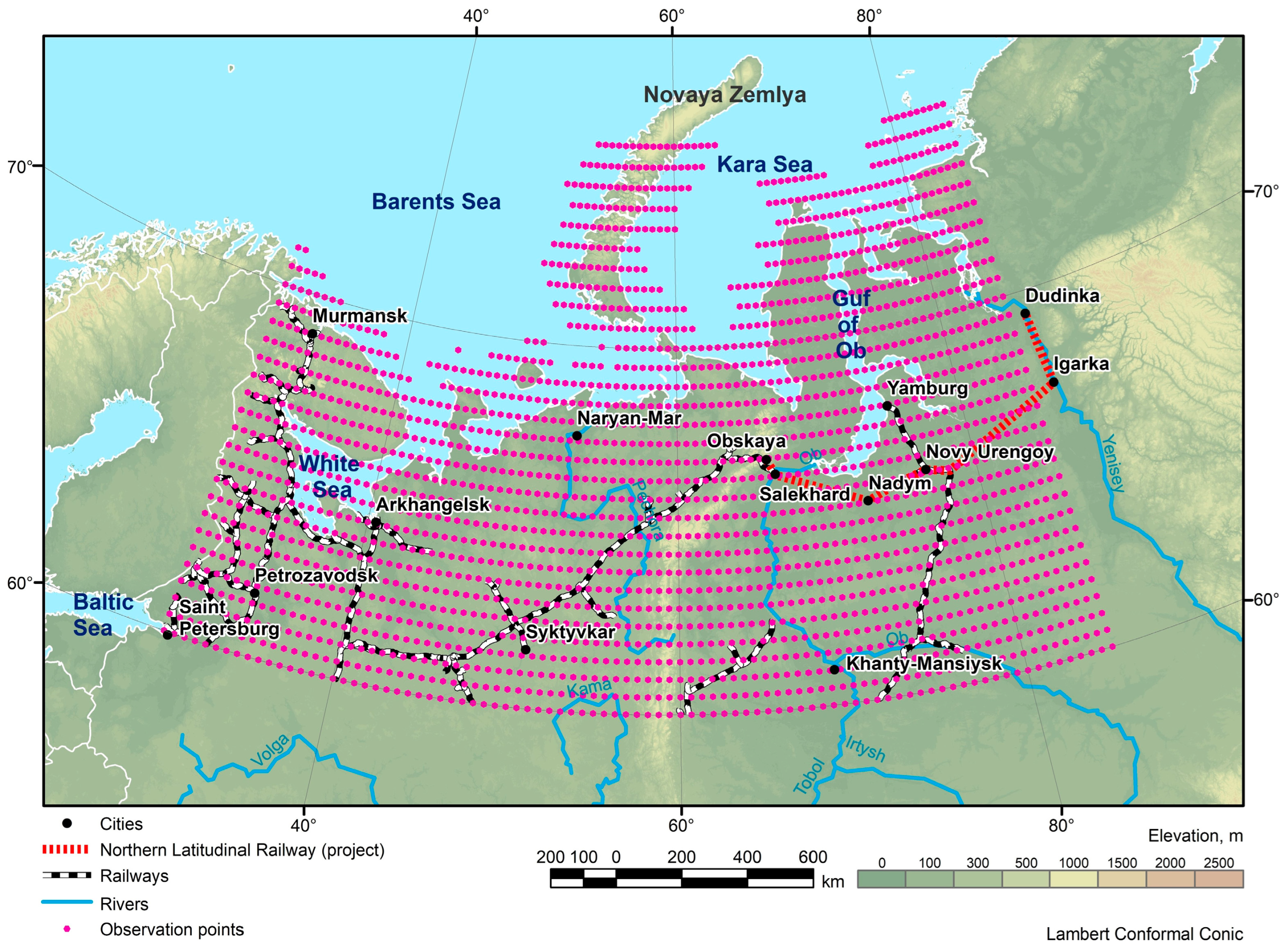
Let us describe the main groups of the resulting maps and the ways of processing the information for their construction. For each of the parameters, the input data are digital arrays containing the coordinates (with a spatial resolution 0.5° × 0.625°) and parameter values. These arrays are further structured by time intervals: for main parameters from 1950 to 2021, and for auxiliary parameters from 1980 to 2021.
While calculating various characteristics, the used data had certain time sampling, which was as follows:
  • 1950–2021—the entire time interval according to NCEP/NCAR Reanalysis 1;
  • 1980–2021—the entire time interval according to MERRA-2 reanalysis data;
  • 1980–1999—period when the observed values were less accurate (according to MERRA-2 reanalysis data);
  • 2000–2021, the period with the best resolution and modern observation system (according to MERRA-2 reanalysis data).
By overlaying the information in each file on the grid, the characteristics were calculated in each node of the grid within the defined period [42]. Each grid node contains data averaged for its vicinity ±1.25°.
For the main parameters (air temperature, total precipitation, wind speed), the characteristics were calculated starting from 1950, since these parameters were measured in sufficient detail even before the modern satellite observation network was created. An example of such an initial digital map is shown in Figure 10.
For each combination of climatic parameters, the following groups of characteristics were calculated when creating the initial digital map:
  • Arithmetic means for individual time periods;
  • Average parameter changes between the periods 1980–1999 and 2000–2021;
  • Average values for each month separately (12 maps);
  • Average values by season: summer (June–August), and winter (December–February);
  • Average values between the periods 1980–1999 and 2000–2021 for each month;
  • Average values between periods 1980–1999 and 2000–2021 by season—summer (June–August), and winter (December–February);
  • Average rate of change of mean monthly characteristics.
The anomalies shown on the maps for different months allow us to distinguish local changes, as well as to correlate different parameters in time. In this group, the average values are taken as a sample for each day of a certain month for each year of the selected time interval.
Since the studied area is the northwestern part of Russia, this zone is characterized by strong temperature fluctuations and, consequently, by strong changes in other parameters. The seasonal analysis makes it possible to trace the intra-annual variability of the parameters.
Moreover, there are the maps of differences in values of individual parameters between the periods 1980–1999 and 2000–2021. As this group initially carries information about anomalies for the two certain periods and compares them, it allows for not only tracing regional changes of climatic parameters, but also giving a quantitative assessment of climate change on scale of almost half a century.
The rate of change of the specified parameters is calculated as the first derivative over time (X) for the data set in Figure 11 [5]. The rate of change (a) of any parameter (Y) was calculated using the linear regression equation:
Y(X) = a · X + b.
This characteristic of temporal variability allows for defining how fast the studied parameters change.
In total, 459 maps with different characteristics of the specified climatic parameters within the selected time intervals were compiled.

3.2. Air Temperature

Air temperature is the parameter that reflects the degree to which air is heated. Historically, air temperature was one of the first climatic parameters that scientists began to measure. When satellite missions were launched, they began to measure atmospheric temperature at various altitudes, e.g., sea surface or land surface. The most common method for satellite measurements is obtaining data using radiometric sounding. For this purpose, instruments that measure radiation in different wavelength ranges, most commonly infrared radiation allowing for calculating the temperature at specified heights, have been developed. The MERRA-2 reanalysis used upgraded instruments to measure vertical profiles of parameters such as air temperature and humidity—the CrIS Cross-Track Infrared Sounder (CrIS) and the Advanced Technology Microwave Sounder (ATMS) [19].
The CrIS Cross-Track Infrared Sounder is one of the most advanced hyper spectral instruments in the National Oceanic and Atmospheric Administration (NOAA) Joint Satellite System. CrIS is a high-resolution infrared spectrometer of which the operating principle is based on the separation of infrared energy emitted by the atmosphere, resulting in high vertical resolution. The instrument provides atmospheric sounding within 2,211 spectral channels in three wavelength bands: long-wave LWIR (9.14–15.38 µm), medium-wave MWIR (5.71–8.26 µm), and short-wave SWIR (3.92–4.64 µm) [44].
The Advanced Technology Microwave Sounder (ATMS) is a 22-channel scanning microwave radiometer for atmospheric and Earth surface observations, which makes observations in the microwave part of the electromagnetic spectrum. ATMS and CrIS provide data on the water cycle, namely, water vapor, clouds, and precipitation. Since clouds are non-transparent in the infrared part of the spectrum (as measured by the CrIS instrument), the two instruments work in combination to cover a broader range of weather conditions. ATMS provides a view inside and under clouds and can be used to study storms and hurricanes from the inside [45].
The MERRA-2 catalog presents temperature values for various altitudes: 2, 10, 42, 72 m, and at “surfaces” where atmospheric pressure is 250, 500, and 850 hPa. The atlas used air temperature values at 42.2 m above the ground surface. This makes it possible to analyze the data without taking into account the influence of wind, snow, and other surface factors.
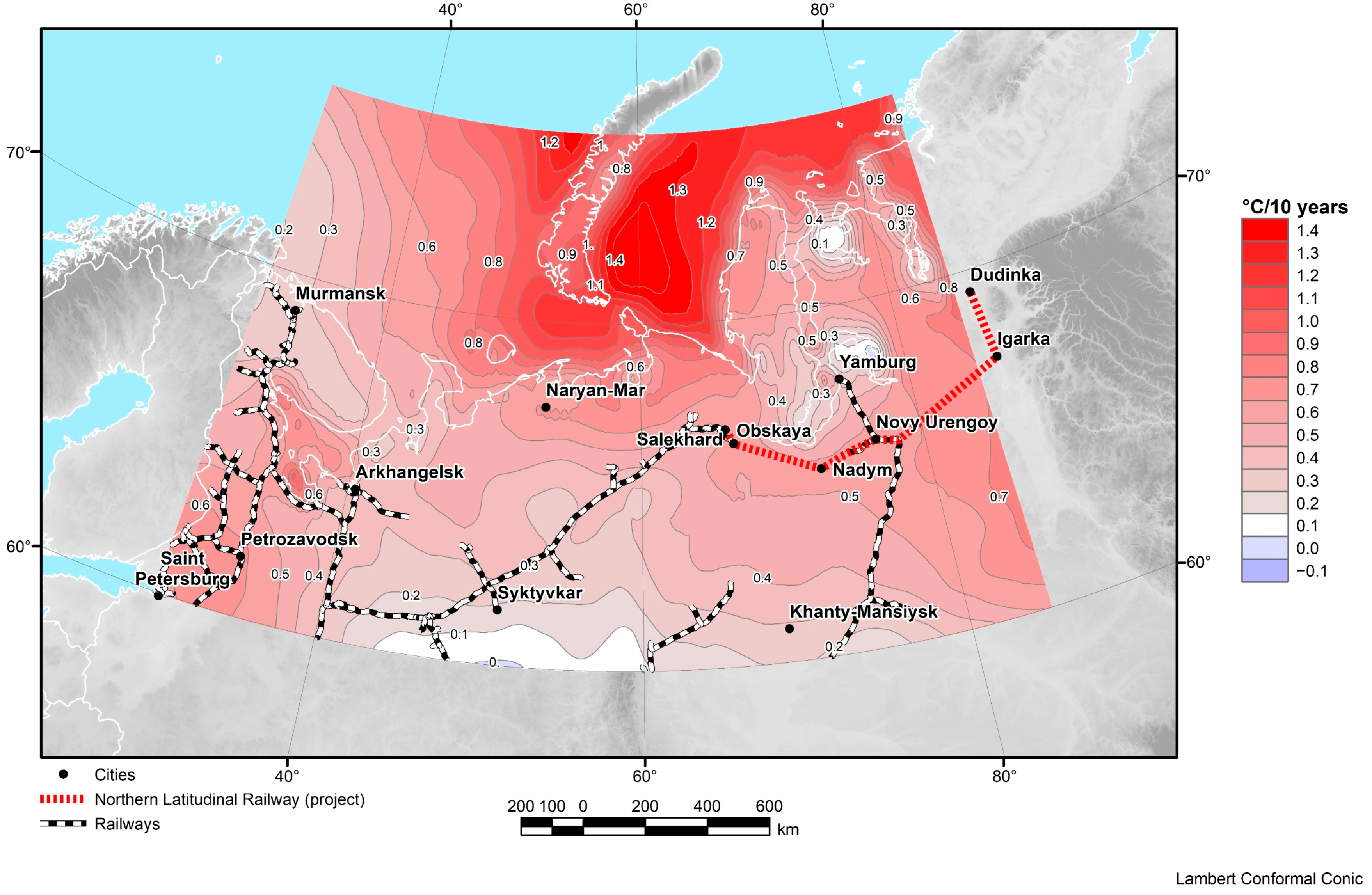
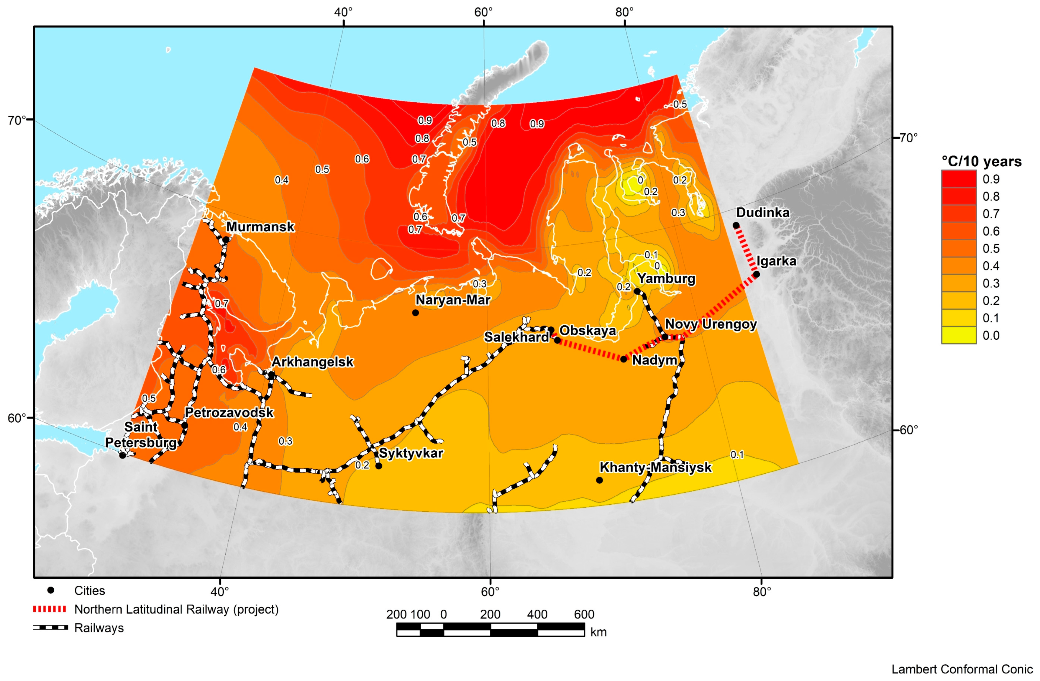
If we use the compiled maps for the purpose of climate forecasting, the general tendency of average air temperature increase since 1980 is clearly observed in Figure 12. This map shows the rate of change of the average annual air temperature. All values are positive, which means that for the specified time period, the temperature values are exclusively increasing. Additionally, we can distinguish the general trend—the more northward, the stronger the temperature changes are. In the area of the Novaya Zemlya Archipelago, the values of average annual temperature increase by 1 °C per 10 years.
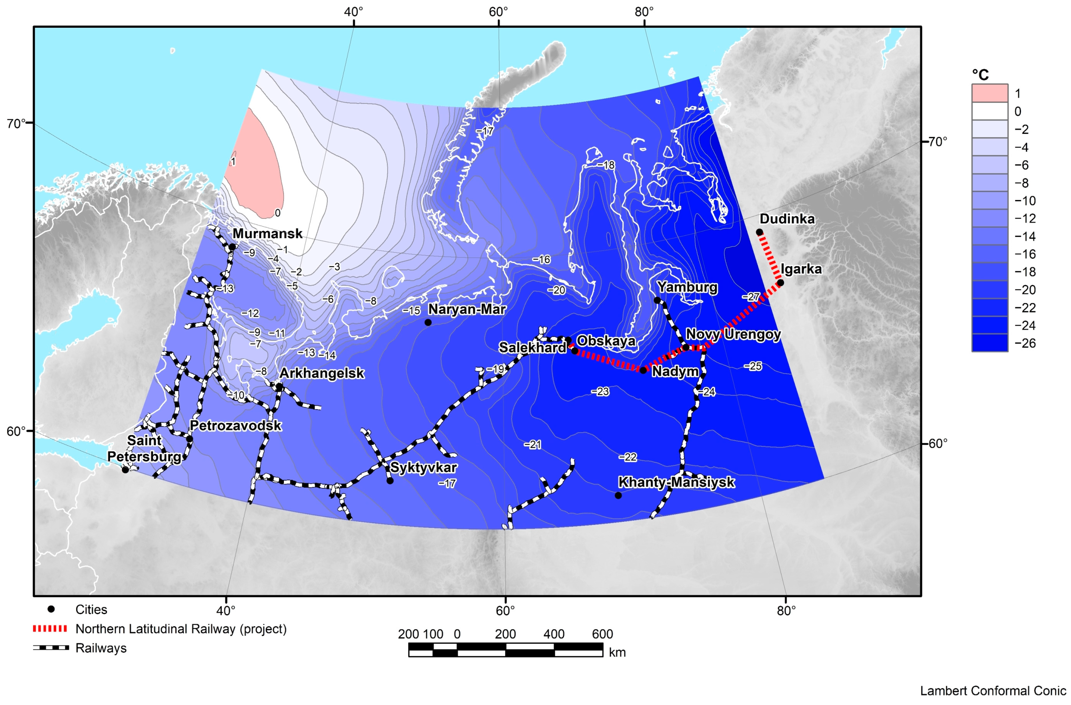
Since the studied area is located in the north, we can note extreme temperature values in winter periods, as well as characteristic areas where the cooling is not in contrast. Figure 13 shows a map of air temperature values for the whole period for January. The data indicate that the general trend of decreasing temperatures is directed from west to east—from near-zero temperatures north of the Kola Peninsula, to −26 °C in Taimyr and from −20 °C to −24 °C in Siberia. Zero temperatures, however, are present only in the oceanic part of the territory, which is explained by the influence of warm ocean currents. On land, this influence disappears, and temperatures range from −8 °C to −10 °C.

3.3. Total Precipitation

Precipitation is a value that describes the height, in millimeters, of a water layer that would form on the surface of the Earth without external influence. The first measurements of this parameter were made for the purpose of storm analysis, rain distribution, and rainfall forecasting. The first satellite measurements of precipitation were made using radar to produce three-dimensional maps of storm structure and to calculate the altitudes where the phase transition from snow to rain occurs. Since one of the most important climatic processes is the water cycle on Earth and in the atmosphere, such data allowed qualitatively to complement and improve models of global atmospheric circulation. The most common methods of precipitation measuring nowadays are either microwave sensors or ground-based observatories. Microwave sensors measure the energy emitted by the atmosphere or the ground, and extract quantitative characteristics of water vapor, water in clouds, and the intensity of precipitation in the atmosphere from the signal. There are sensors that additionally allow estimating both the rate of precipitation and the geometric characteristics of water particles.
The MERRA-2 reanalysis mainly contains data from ground stations, collected in the Global Historical Climatological Network (GHCN) database, and in the Climate Anomaly Monitoring System (CAMS) database. In these catalogs, there is a basic division of information by ground and ocean stations, which is compared in parallel with similar published data sets from satellite missions.
In the reanalysis, there is a separate processing block to account for inter-annual variability in ocean evaporation [46,47].
It is also worth noting that MERRA-2 initially uses precipitation data based on ground-based observations, which are further archived as an output variable and input parametrically to values obtained from satellite data. A description of the satellite instruments obtaining atmospheric precipitation values is given above in Section 2.2. In addition, some observation areas use CMAP satellite sensor results due to limitations in available observations [48].
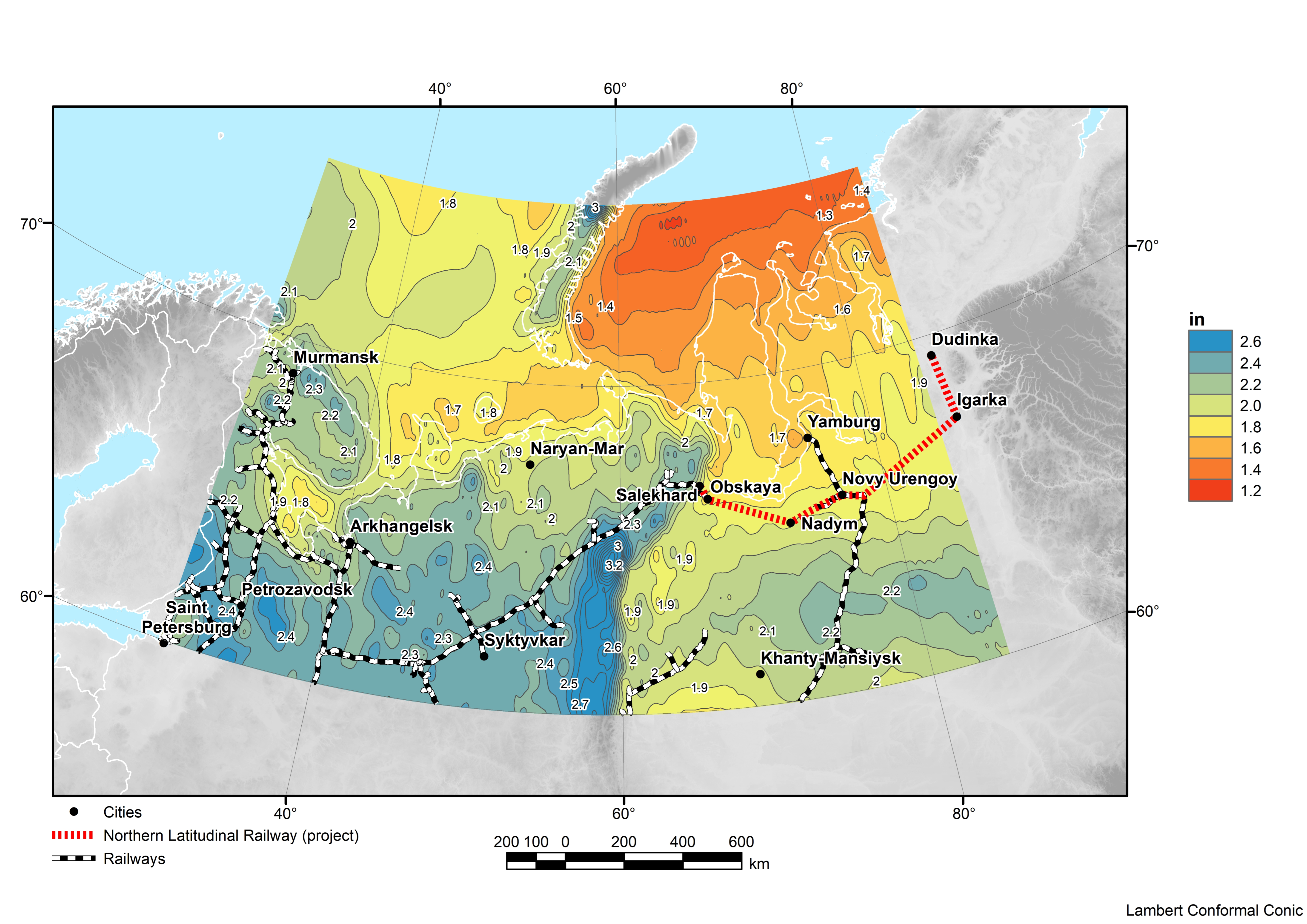
Consequently, the results are provided in the following variations: maximum and minimum precipitation rates for the period, total precipitation, convective precipitation, large-scale precipitation, snow, total precipitation from the atmospheric model, evaporation totals, and corrected large-scale and total precipitation. The adjusted total precipitation data were used in Figure 14. This map clearly identifies the zone with the maximum amount of precipitation, belonging to the zone of the Ural Mountains, and the minimum values are confined to the water area of the Kara Sea.

3.4. Wind Speed

Note that in satellite measurements of wind speed, this value is decomposed into orthogonal components—east and north. Using them, the total vector of wind speed is determined. The measurement methods are often similar to scattermeter devices, the principle of which is based on the reception of signals reflected from the sea surface, and further analysis of the intensity of the reflected wave [14].
Since the wind speed value is not only a climatic parameter, but also a parameter for introducing corrections to other parameters, the MERRA-2 reanalysis uses sensors from both ground-based observatories (UCAR and NCEP) and data from a large number of satellite systems [49]:
  • AVHRR atmospheric motion vector, 1 October 1982–present, CIMSS;
  • SSM/I surface wind speed, 9 July 1987–4 November 2009, RSS;
  • ERS-1 surface wind vector, 5 August 1991–21 May 1996, ESA;
  • ERS-2 surface wind vector, 19 March 1996–29 March 2011, ESA;
  • QuikSCAT surface wind vector, 19 July 1999–22 November 2009, JPL;
  • MODIS atmospheric motion vector, 2 July 2002–present, CIMSS and NCEP;
  • SSMIS surface wind speed, 23 October 2003–29 October 2013, RSS;
  • WindSat surface wind vector, 13 August 2007–4 August 2012, NCEP;
  • ASCAT surface wind vector, 15 September 2008–present, NCEP.
The MERRA-2 catalogs have wind velocity values available for two vectors (meridional and zonal wind) at 2, 10, 50, and 72 m altitudes, at the daytime surface, and at “surfaces” where pressure is 250, 500, and 850 hPa [
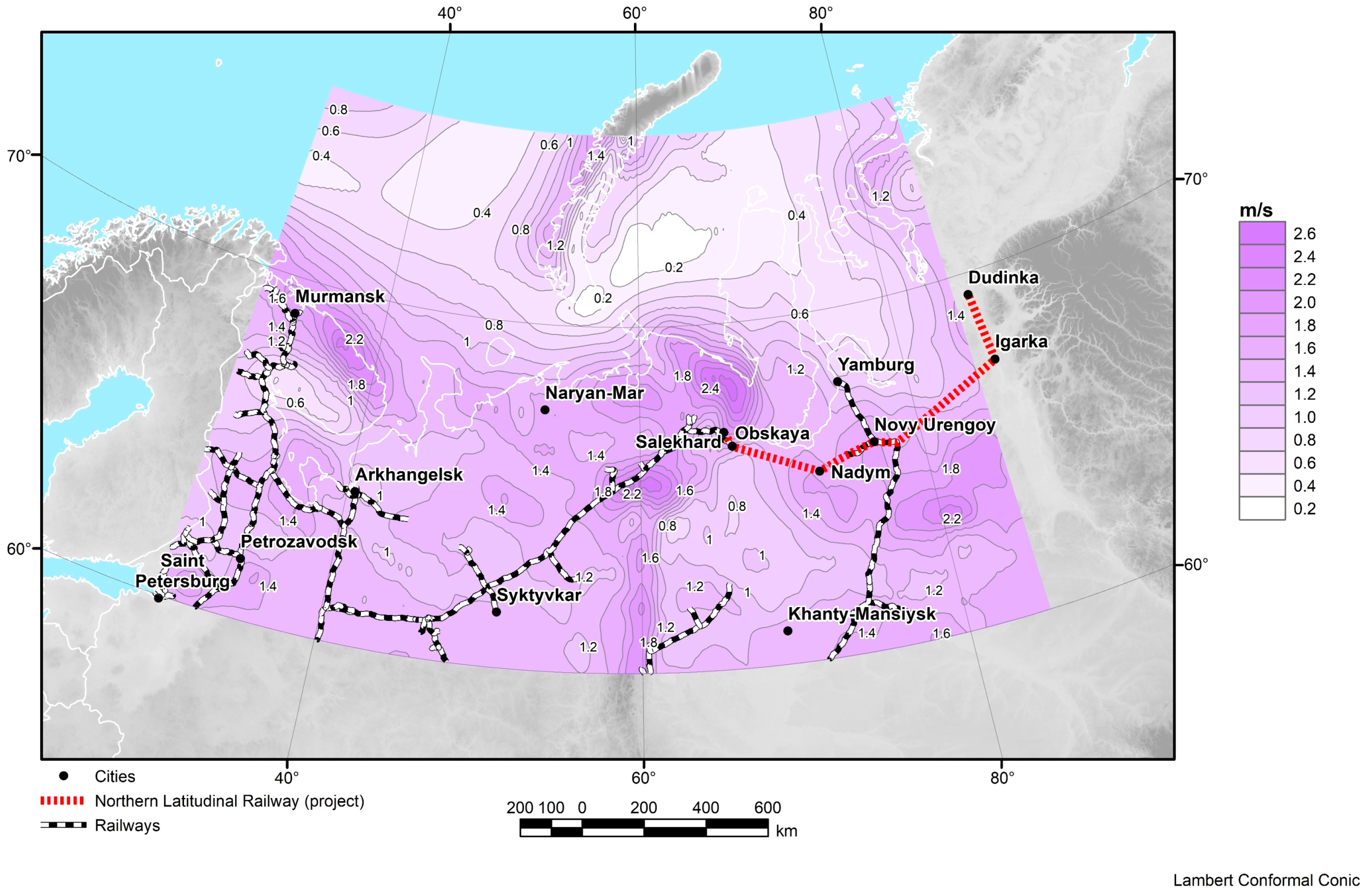
48]. There is also information on trends in inter-annual zonal and meridional wind variability. The atlas presents various wind speed characteristics at 50 m altitude. One of the maps is shown in Figure 15, and displays the average wind speed for the entire time interval (1980–2021).
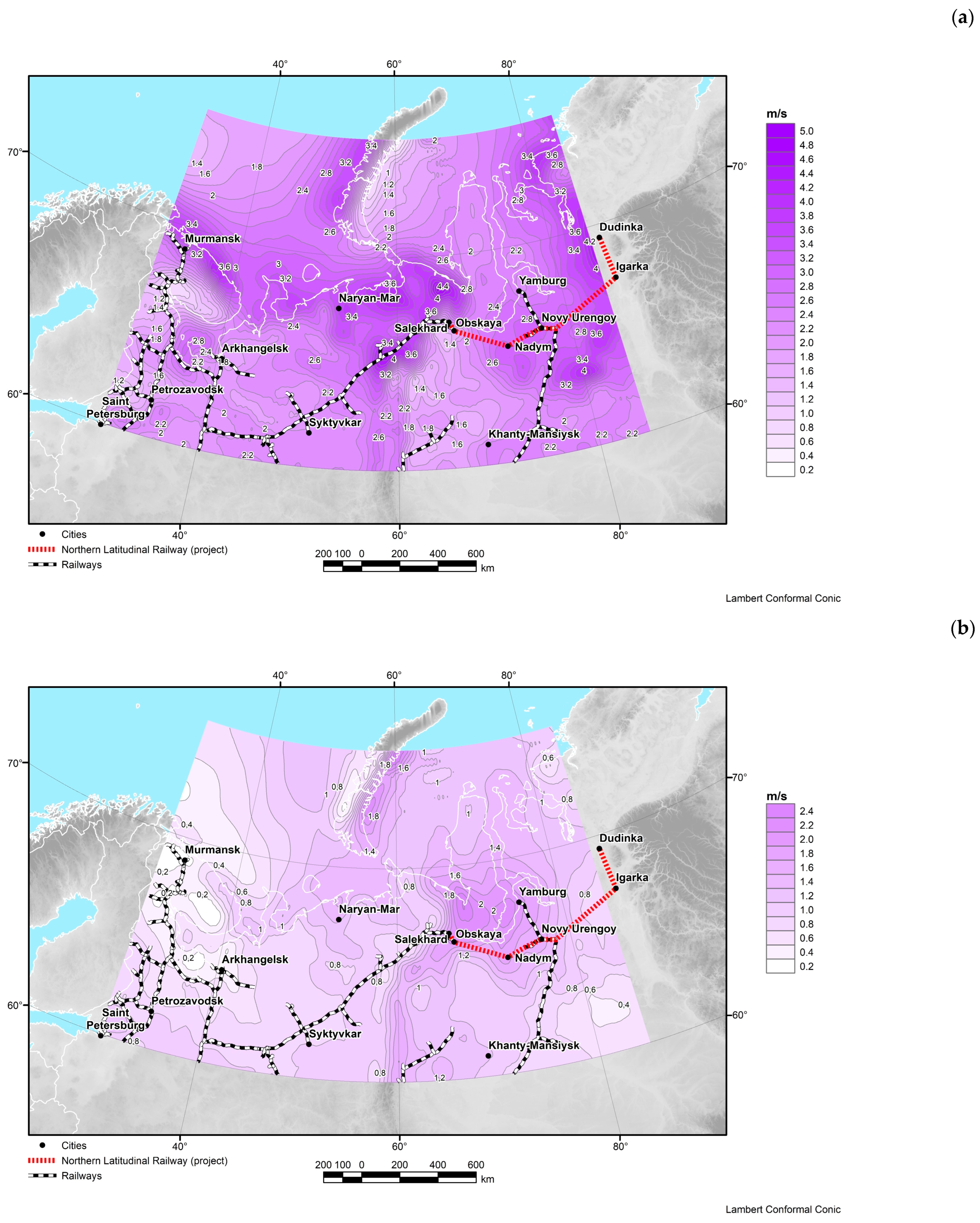
Analysis of average wind speed by months showed a strong seasonal dependence—the highest speeds up to 5 m/s in winter (extremes in December) in Figure 16a and the lowest speeds in summer—values up to 0.4 m/s and less in the regions of the White Sea and Arkhangelsk in Figure 16b.

3.5. Soil Temperature

Soil temperature is a characteristic of the soil upper layer (up to the first meters), reflecting the temperature in a layer of selected thickness. There are special thermometers and remote sensing methods for measuring soil temperature. Physically, the devices emit a signal, which is subsequently recorded by sensors after scattering or reflection from the surface.
Soil temperature in MERRA-2 is measured remotely once per hour, which provides observation of short-scale changes in the parameter [50]. The reanalysis presents soil temperature for different layers: 0–0.1, 0–0.2, 0–0.4, 0–0.75, 0–1.5, 0–10.0 m [48]. The atlas presents soil temperature maps of the Arctic zone of the northwestern Russia, where permafrost zoning is quite apparent in Figure 17. The thickness of the measured layer was chosen as a maximum depth of 10 m, because these areas are characterized by short-term temperature changes, affecting the assessment of global trends in the parameter.

3.6. Soil Moisture Content

Soil moisture content is the percentage of water in the soil compared to dry soil.
For satellite observations, radar and a radiometer are required to obtain an adequate solution. For the MERRA-2 system, soil moisture data were provided using the Soil Moisture Active Passive Observatory (SMAP) system, which is a radiometric and radar instrument.
The approach to soil moisture measurement uses a combination of the radar spatial resolution and the radiometer accuracy with simultaneous measurements of surface radiation and backscattering. Instruments measure parameters in the upper layers of soil to provide a global assessment of the soil moisture. Since some parts of the land are heavily covered with vegetation, the calculations include an automatic algorithm for extrapolation between the values obtained at different times of the day at different positions of the satellite relative to the Earth’s surface.
The final reanalysis data provide soil moisture values in different units [51]. The first is in dimensionless units of relative saturation for different layer depths. The second is soil moisture content in volumetric units of m3/m3, considered as the volume of water in the soil volume (including all solid material, water, and air). In both cases, soil moisture variables are provided for the top 0–100 cm layer. Summary data are also presented for different soil layers, 0–5, 10–100, and 134–853 cm [48]. An example of the soil moisture values is shown in Figure 18. The atlas includes 63 different soil moisture characteristics based on the analysis of data for the period 1980–2021.
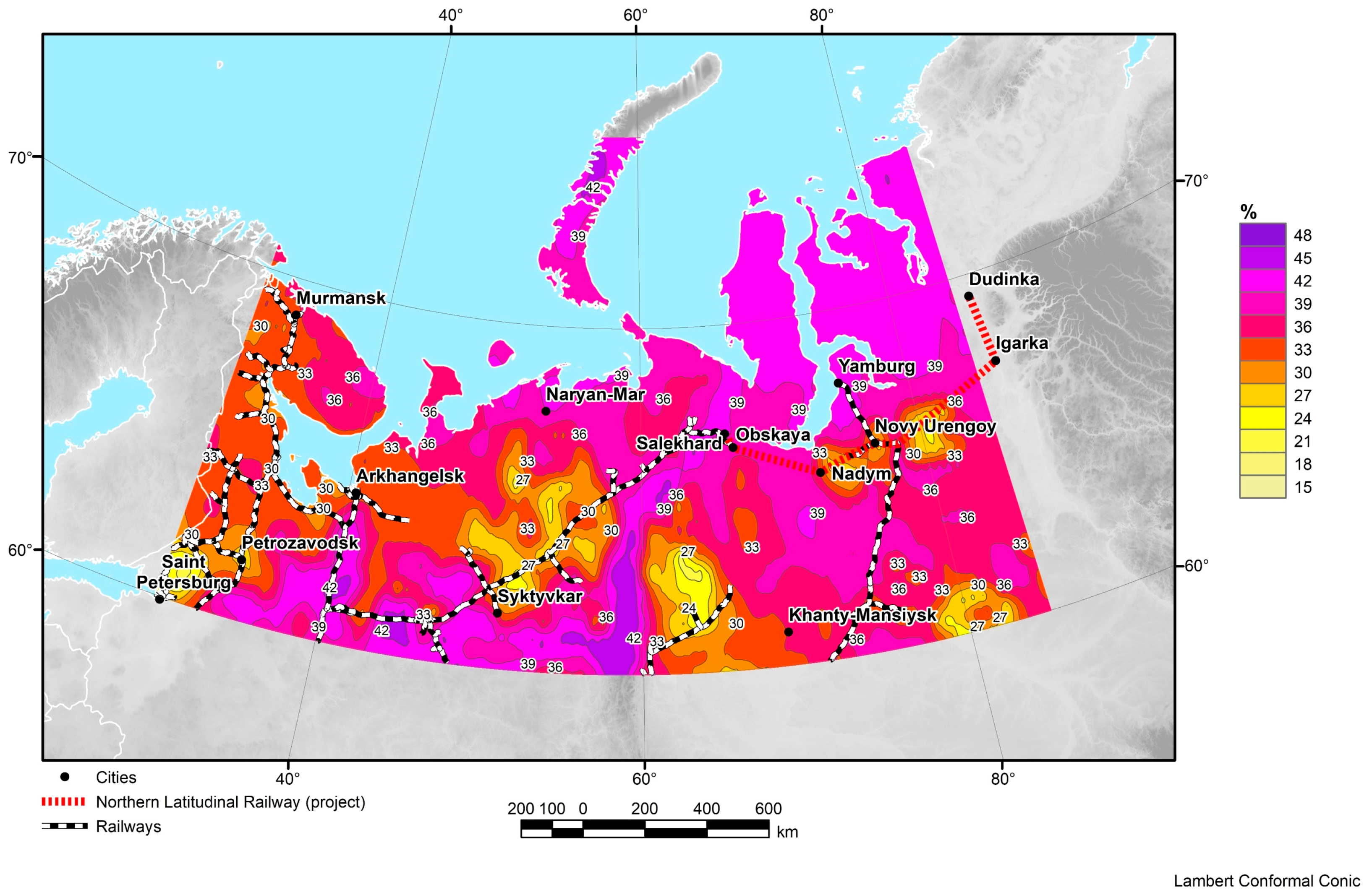
3.7. Air Humidity

Air humidity characterizes the water vapor content in the atmosphere. The MERRA reanalysis used pseudo-relative humidity [52], which was determined through the ratio of water vapor mixing to saturation value.
However, MERRA-2 uses a new approach—the normalized pseudo-relative humidity [53], which is determined by normalizing the pseudo-relative humidity to the standard deviation of the background error, which has a near-Gaussian distribution. Physically, MERRA-2 produces consistent time series of the total amount of water in the atmospheric column and the transport of water from the ocean to the land.
It is possible to obtain types of air humidity as output parameters in the atlas, such as effective specific humidity at the surface, specific humidity using mixed estimation, relative humidity, estimates of the general trend of humidity, and humidity at different heights: 2, 10, 42, 72 m, and at “surfaces”, where the pressure is 250, 500, and 850 hPa [48]. An example of the air humidity distribution is shown in Figure 19. The atlas presents an array of maps for specific air humidity at 2 m.

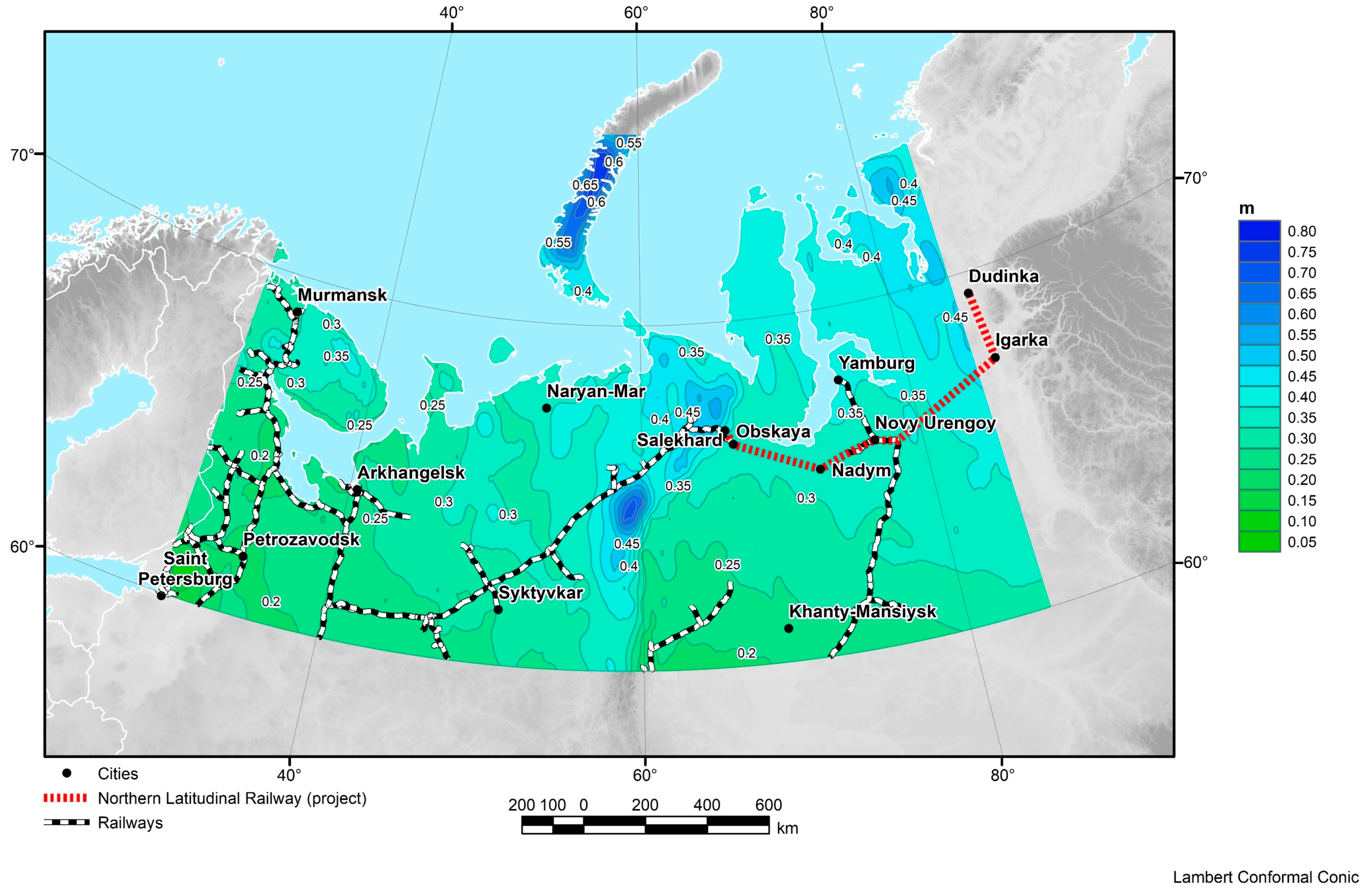
3.8. Snowcover Thickness

The thickness of the snow cover is commonly referred to the thickness of the layer of snow covering the surface of the ground. When measuring the snow cover thickness, there is a need for additional adjustments, which must take into account the characteristics of the snow. It is necessary to measure the thickness of the already compacted layer, and not at the moment of fall, when the melting process in the outer medium is possible. A solution to this problem is presented in [54], where a comprehensive dataset for the northern hemisphere on permafrost with a resolution of 81 km is evaluated. The snow cover thickness available in MERRA-2 is recorded only within the territory covered with snow [55]. The reanalysis presents characteristics such as the snow cover adjusted with displacement, total snow mass, snow mass above the ice surface, and snow thickness [48]. The atlas presents various characteristics of snow thickness in meters, e.g., the average values of snow cover thickness in Figure 20.
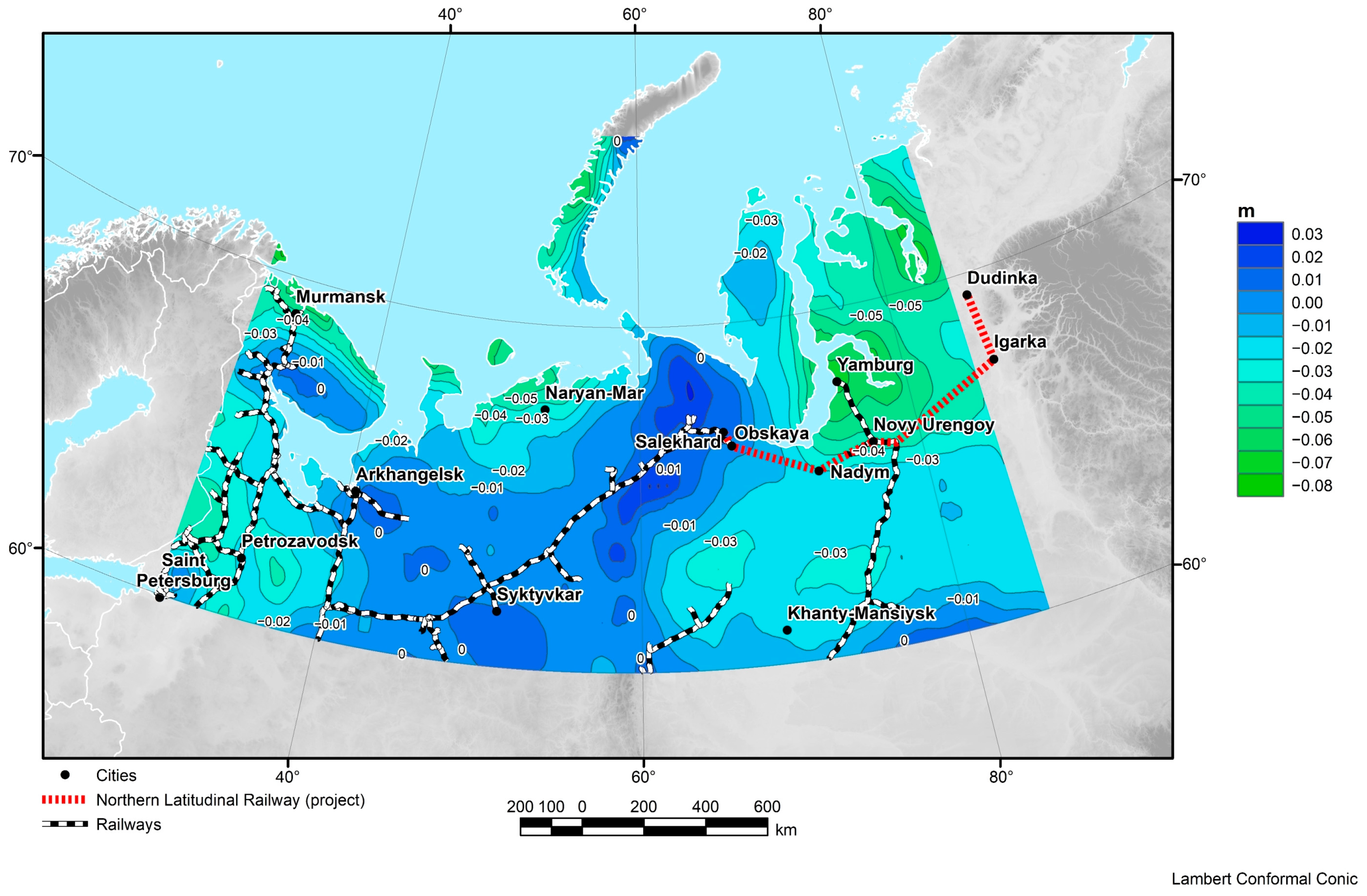
Additionally, it is possible to analyze the change in the thickness of the snow cover in the Arctic zone. Figure 21 presents a map of the difference in snow cover thickness between 1980–1999 and 2000–2021. The difference in the average values of snow cover thickness between the periods allows us to conclude that in the western and eastern parts of the studied area, as well as along the coast of the Barents Sea, there is a decrease in snow cover thickness up to 10 cm, while in the central part there is a slight increase—up to 2 cm.

3.9. Auxiliary Data-Layers of the Atlas

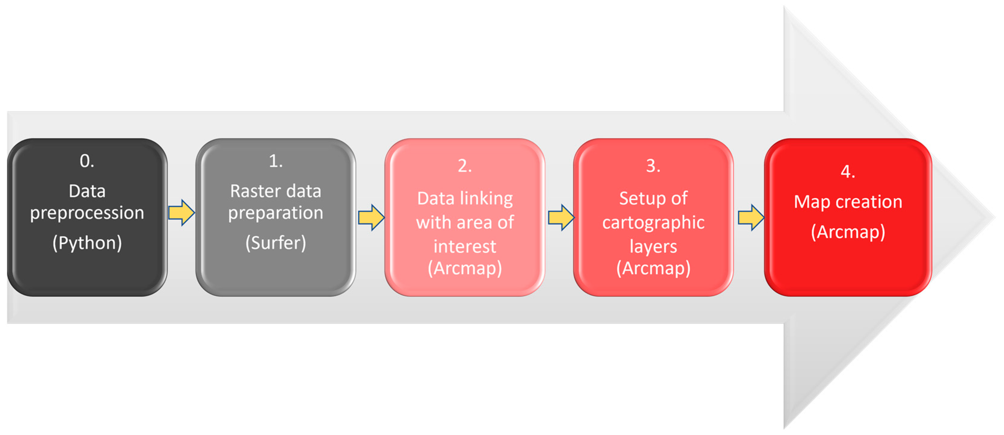
Auxiliary data were employed for filling the atlas maps with additional layers to facilitate the visual assessment (more accurate determination of objects’ location within the map). Such information included physical and geographical parameters, administrative regions, and infrastructure objects. All operations on employing the auxiliary data were performed in ESRI ArcGIS (ArcMap) software. Let us consider this auxiliary information.
The physical map of Russia was used as the base for compiling the atlas maps. It includes topographical features of the regions of the western part of the Russian Federation: Northwestern Federal District (NFD), and Ural Federal District (UFD). The most suitable digital representation (at a scale 1:2,500,000) was provided by the Karpinsky All-Russian Research Geological Institute (VSEGEI). Digital geographic bases were prepared using ESRI ArcGIS software in conic equidistant projection [56,57].
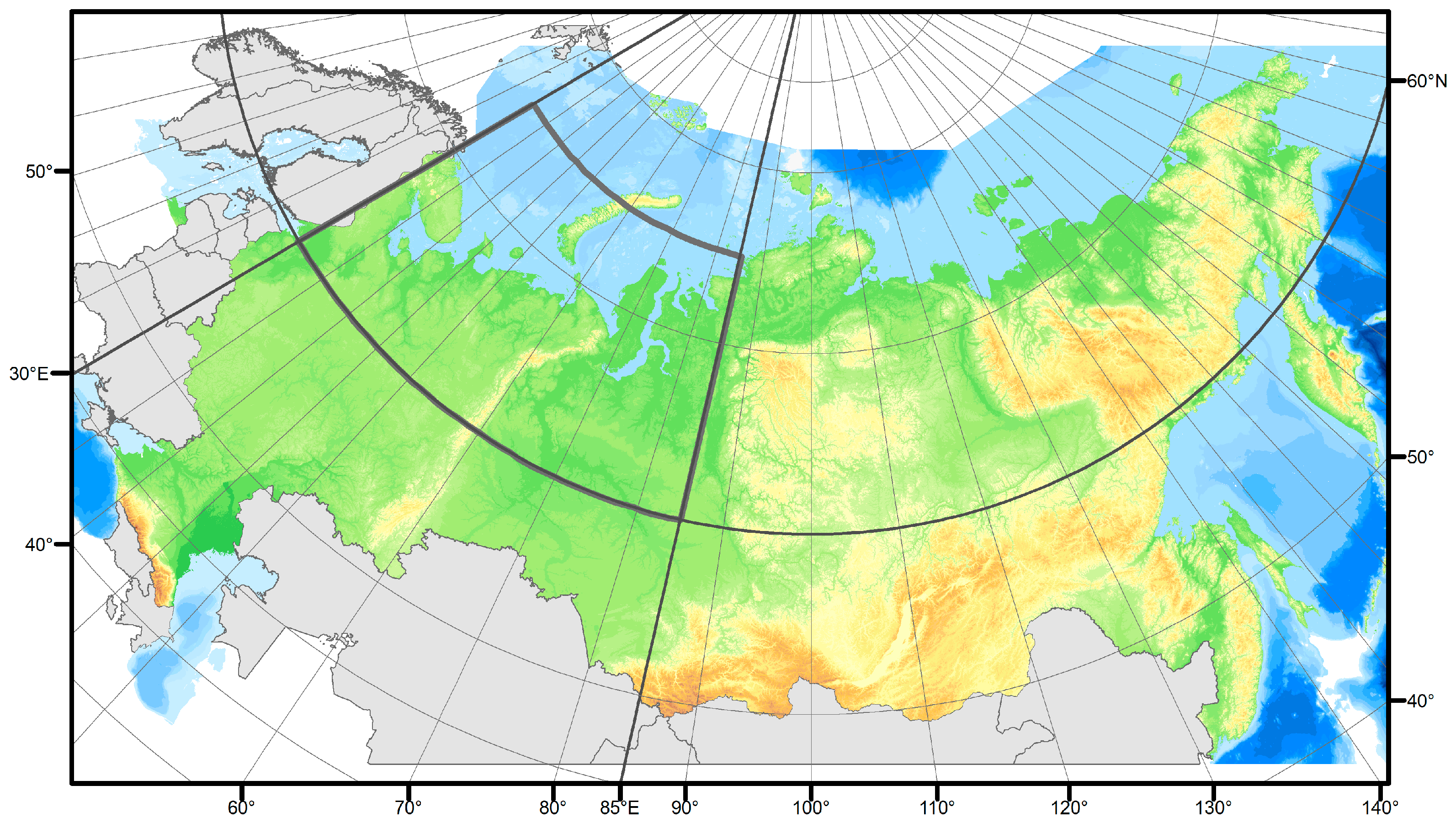
The digital elevation model (DEM) was added to display the main terrain and relief features of the studied area. Considering the wide coverage of the territory, as well as high resolution, the GEBCO DEM with 30 m resolution was selected. The data is a global DEM for ocean and land showing elevation and depth in meters, on a grid with an interval of 1 angular second (about 30 m) [
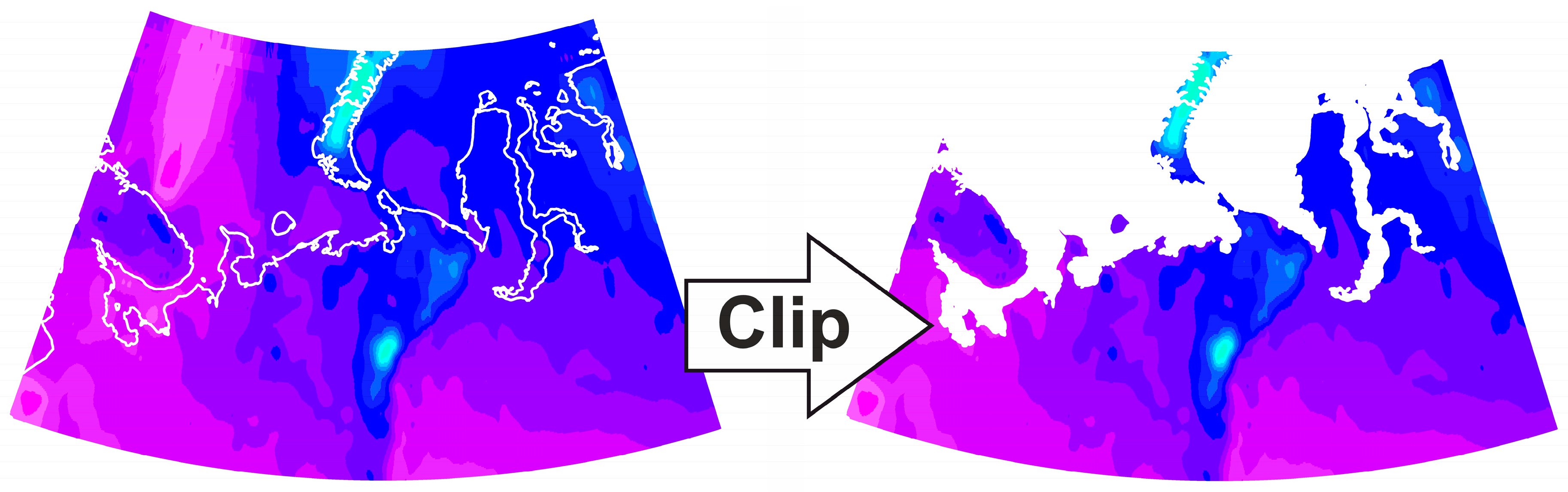
58,59]. The model at first was cropped to the territory of the Russian Federation, then to the boundaries of the studied area as part of this work.
Since there are only six administrative centers of the Russian Federation regions within the studied area, in order to increase the level of detail of the atlas maps, it was decided to also include the basic information on the settlements with a population of over ten thousand people [60]. The initial database includes: the name of the settlement, population, coordinates, administrative codes, and other information. The database was transformed into vector point geodata, and then cropped to the studied area.

4. Discussion

In this section, we discuss only those results which, from our point of view, are the most significant for consideration by railway operators.
Serykh and Tolstikov [42] analyzed climatic changes in air temperature, precipitation, and wind speed in this region. The authors showed that there were significant changes in these parameters between the periods 1980–2000 and 2001–2021. The strongest increase in temperature was observed for November and April, indicating that there was a shift in the time boundaries of the seasons—a later start and an early end of winter. It was revealed that in 2001–2021 the temperature increased most rapidly in the offshore area of the Barents and Kara Seas and this growth was accelerated. We have shown that the detected increase in the amount of precipitation is associated with a significant change in atmospheric circulation in the studied area. In the summer season and in September, there was an increase in the west wind within this territory. In the winter season of 2001–2021, there was an increase in the south wind in the Barents and Kara Seas as compared to 1980–2000.
Serykh and Tolstikov [43] found an increase in upper 1.5 m soil temperatures of about 0.5 °C in 2001–2021 as compared to 1980–2000 in the west of the studied area. This may lead to the reduction and even complete disappearance of the island permafrost on the Kola Peninsula, where average soil temperatures increased almost everywhere in 2001–2021 to +3 °C and more. In 2001–2021, an accelerating increase in soil temperature also began in the northeast of the western part of the Russian Arctic. There was a decrease in snow cover thickness in the west and east of the studied area in 2001–2021 as compared to 1980–2000. In the west of the studied area, there was also a significant reduction in the area of snow cover in November and April. An increase in specific humidity at 2 m altitude began in the west of the studied territory, and especially over the White Sea in 1980–2000. In 2001–2021, the increase in air humidity spread to the center and the east of the studied region with the highest growth rate over the waters of the seas, and this growth occurred with acceleration. These changes can be explained by the increasing influence of the North Atlantic on this territory and this process can be called “Atlantification” of the climate of the western part of the Russian Arctic. This phenomenon may lead to an increase in the number, strength, and duration of extreme weather events in this area [43].
Our research confirms that the warming of this area is significant and occurs in the direction from southwest to northeast [
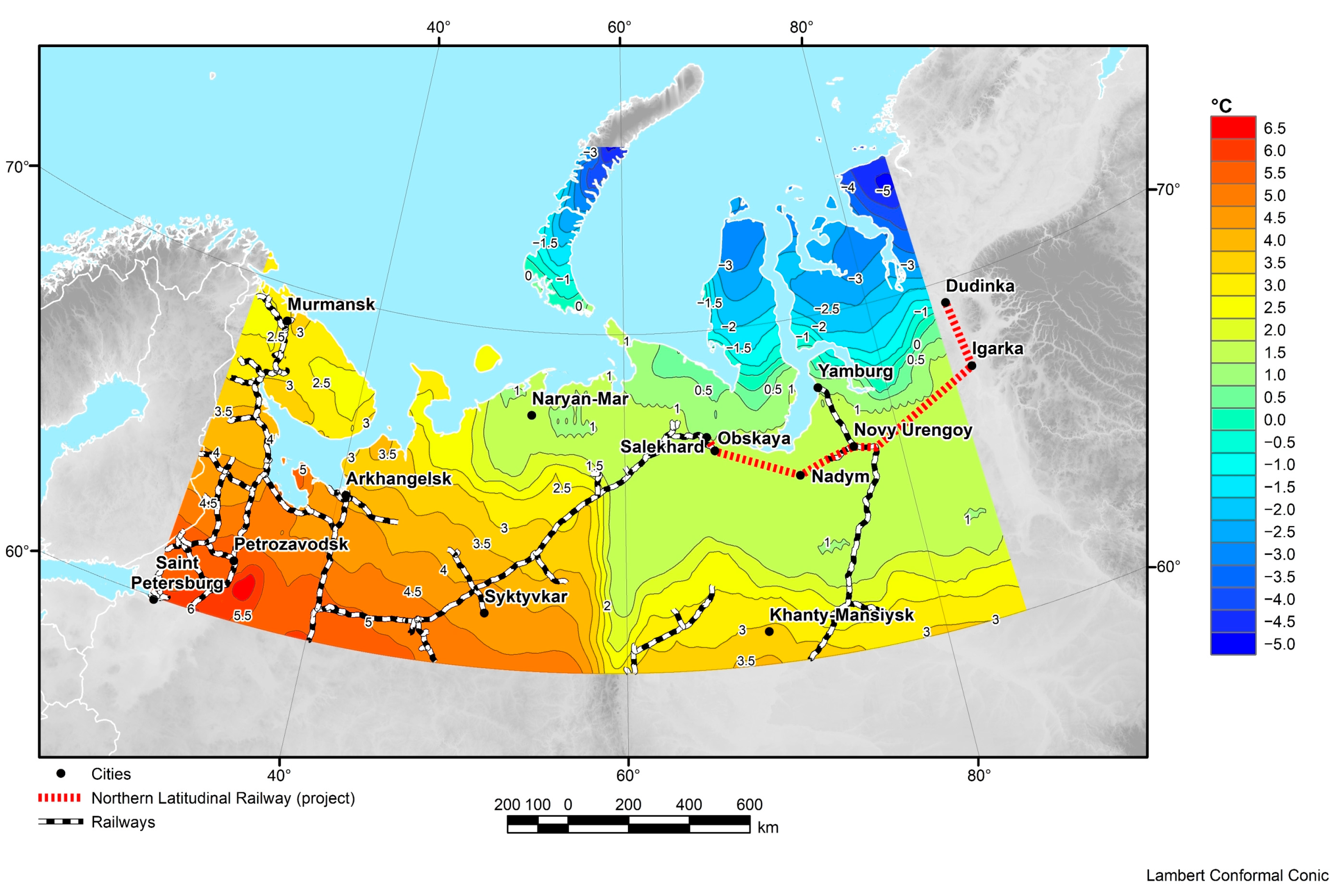
61]. The railway section from Syktyvkar to Salekhard and the section to Yamburg over the past two decades are in an area where average annual air temperatures remain below 0 °C in Figure 10. This means that these sections are operated under difficult weather and climatic conditions for all 12 months (as positive air temperature here is on average only from May to September), and the average monthly air temperature reaches from −20 °C to −22 °C in winter. Warming of the regional climate will occur along these sections, which will lead to thawing of permafrost, change of hydrological characteristics of numerous rivers, lakes, wetlands and may negatively affect the stability of railway tracks and bridges.
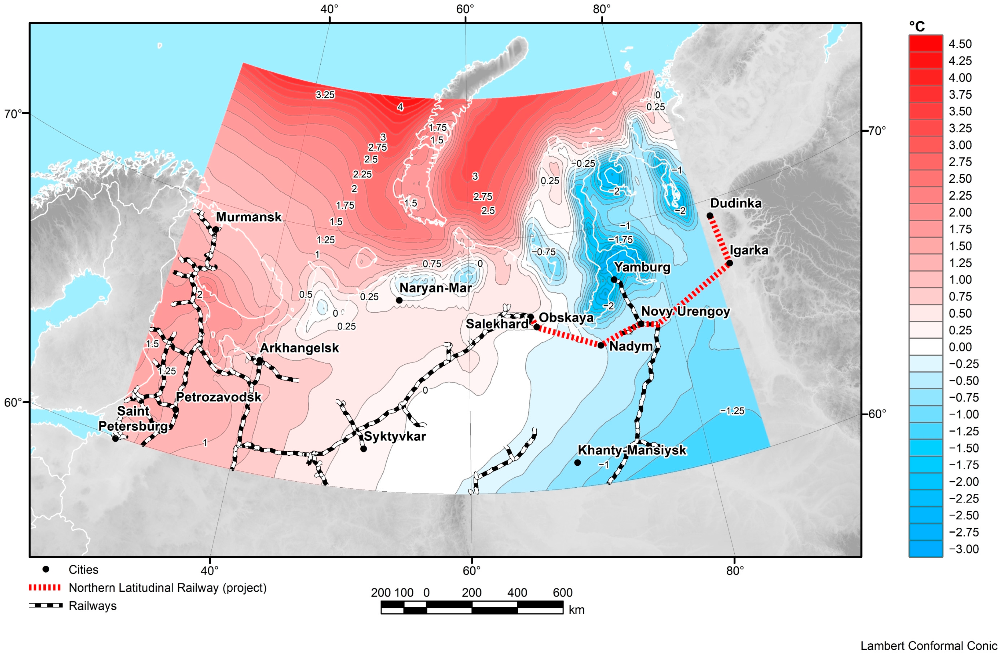
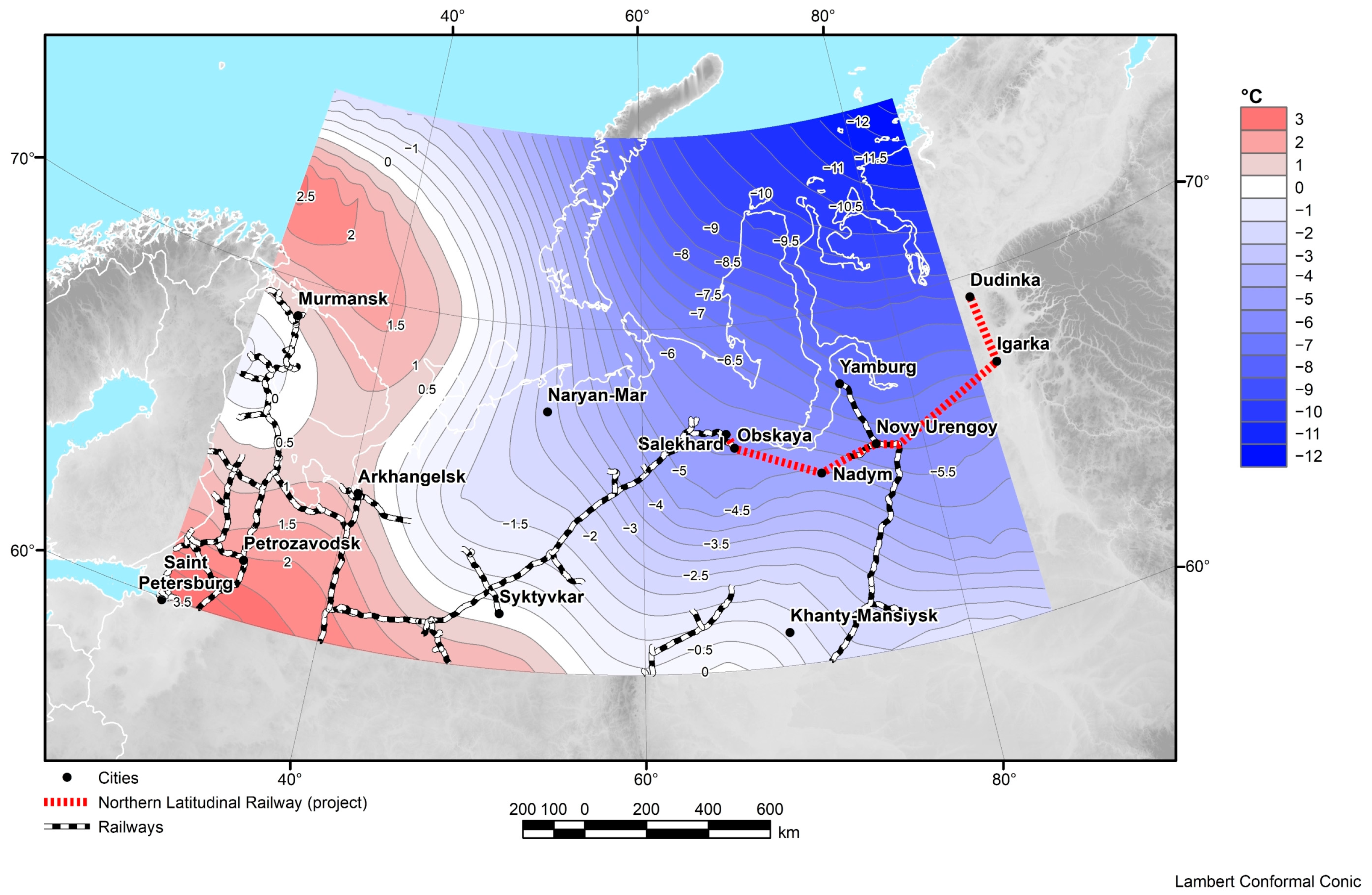
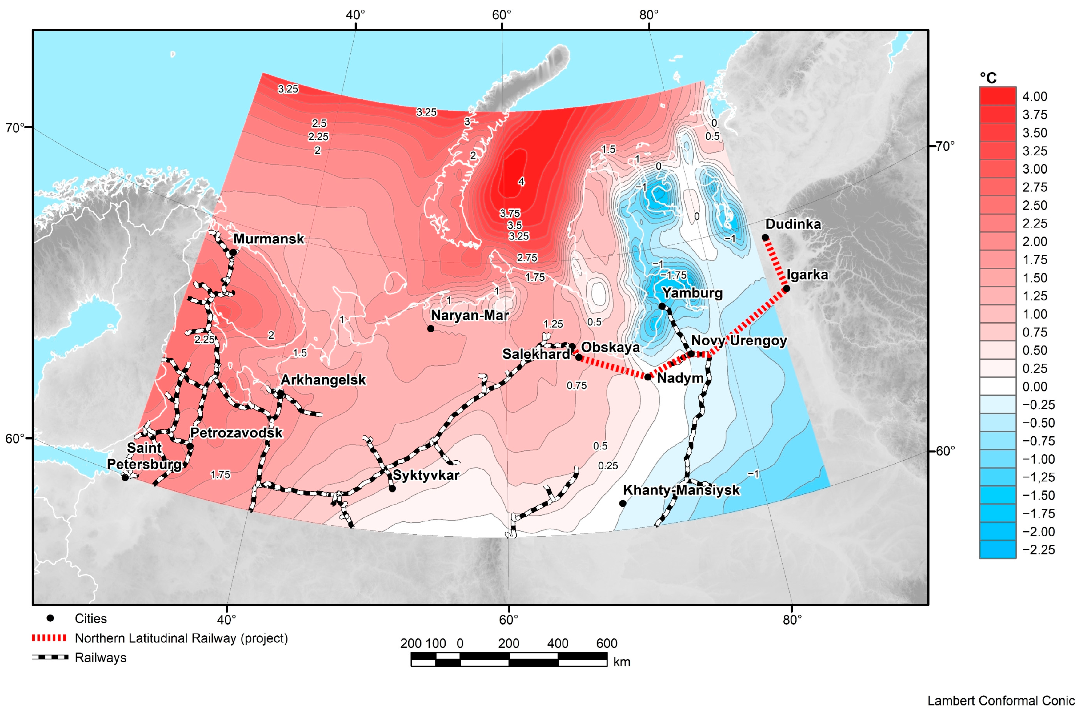
Air temperatures along these railways increased by an average of 0.4–0.6 °C between 1980–1999 and 2000–2021. Comparing these two periods, in January, the warming up to 1.0–1.5 °C was observed along the section to Murmansk and Arkhangelsk, warming up to 0.5 °C was observed along the section to Salekhard, and the cooling of 1–2 °C was observed on the section to Yamburg. In February, warming up to 0.8 °C was observed only on the section to Murmansk. In March, warming to 1 °C was observed only on the section to Yamburg. In April, warming to 1–2 °C was observed along all railway sections, with the warming being greater in more northerly sections. In May, warming to 1–2 °C was observed along all sections of the railways. In June, the greatest warming was observed along the sections to Salekhard and Yamburg, and northwards and eastwards the anomaly was greater, up to 2.4 °C. In July, August, and September, on the contrary, the temperature anomalies in the western part of the studied area were greater (up to 0.8–1.4 °C) than along the eastern sections of the railways. In October, there was a uniform warming of the entire region to 0.8 °C, and only on the northernmost railway section to Murmansk and Yamburg the anomaly reached 1.2 °C. In November, all the sections showed warming between 2 °C and 2.6 °C, except for the section to Yamburg, which reached 0.8 °C. In December, the warming increased from east to west, from 0 °C to 2.2 °C on the section to Murmansk in Figure 22. Thus, the regional climate change is very uneven within the year (by month), spatially, and even along each section of the railway separately.
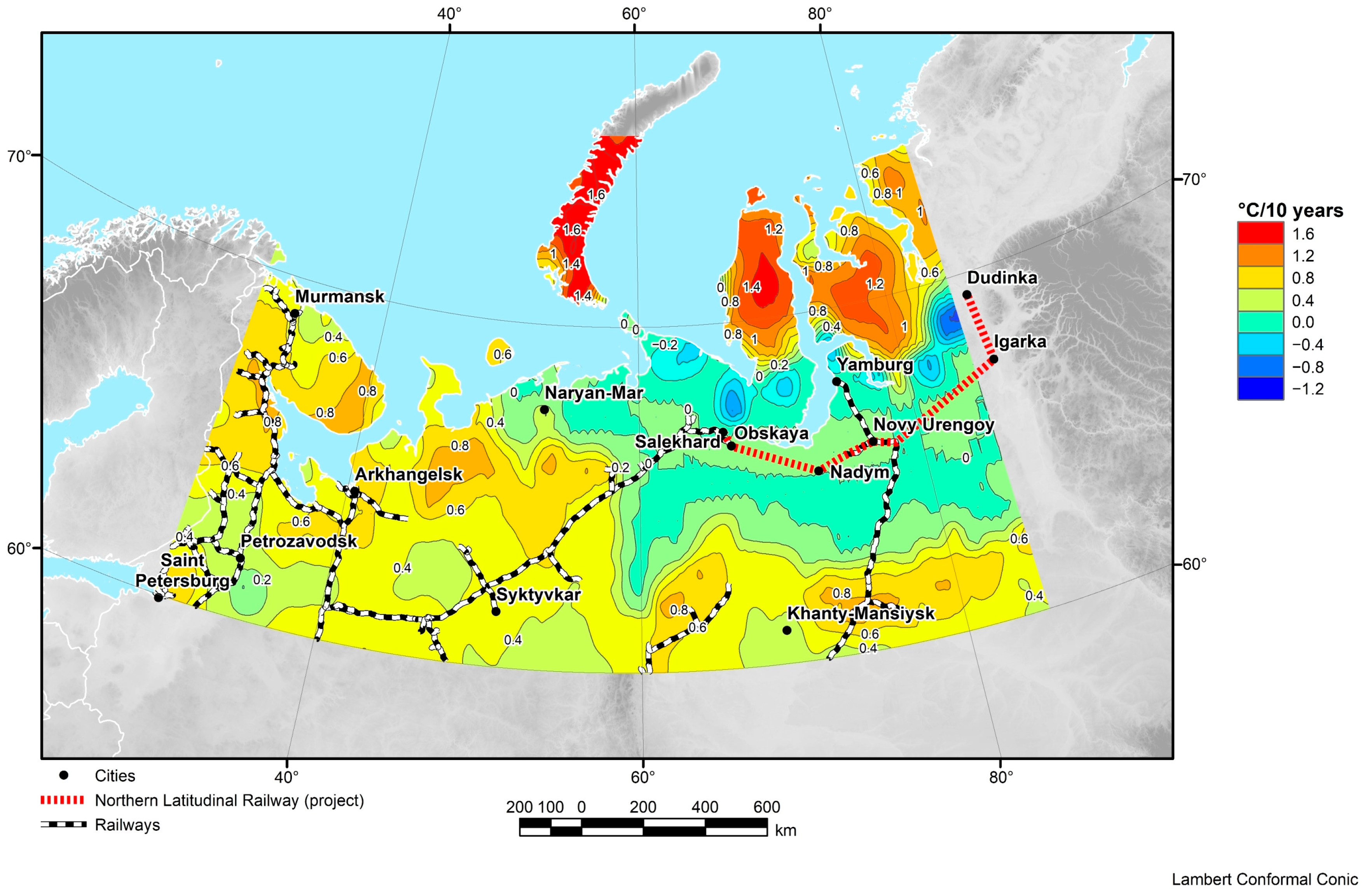
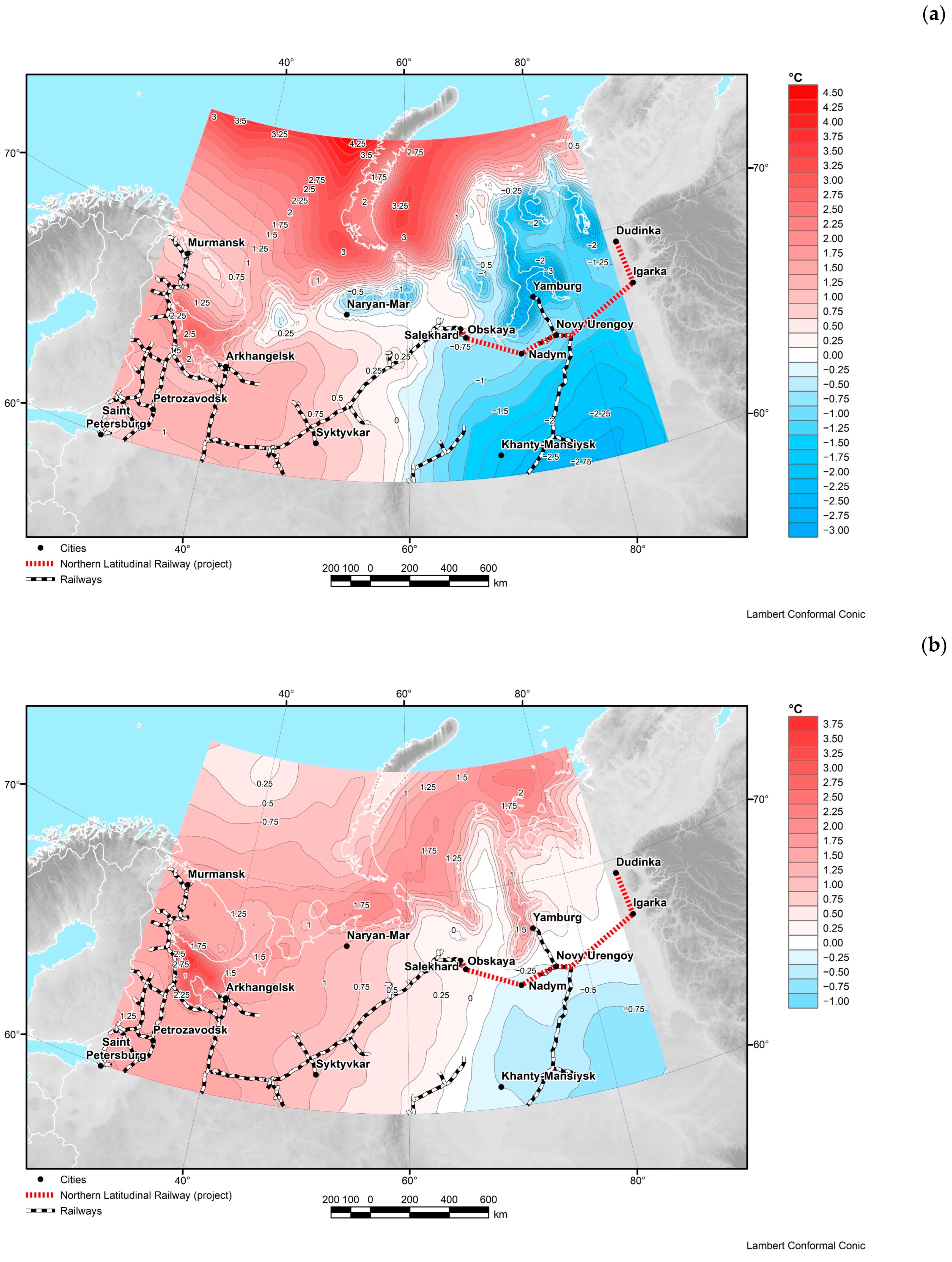
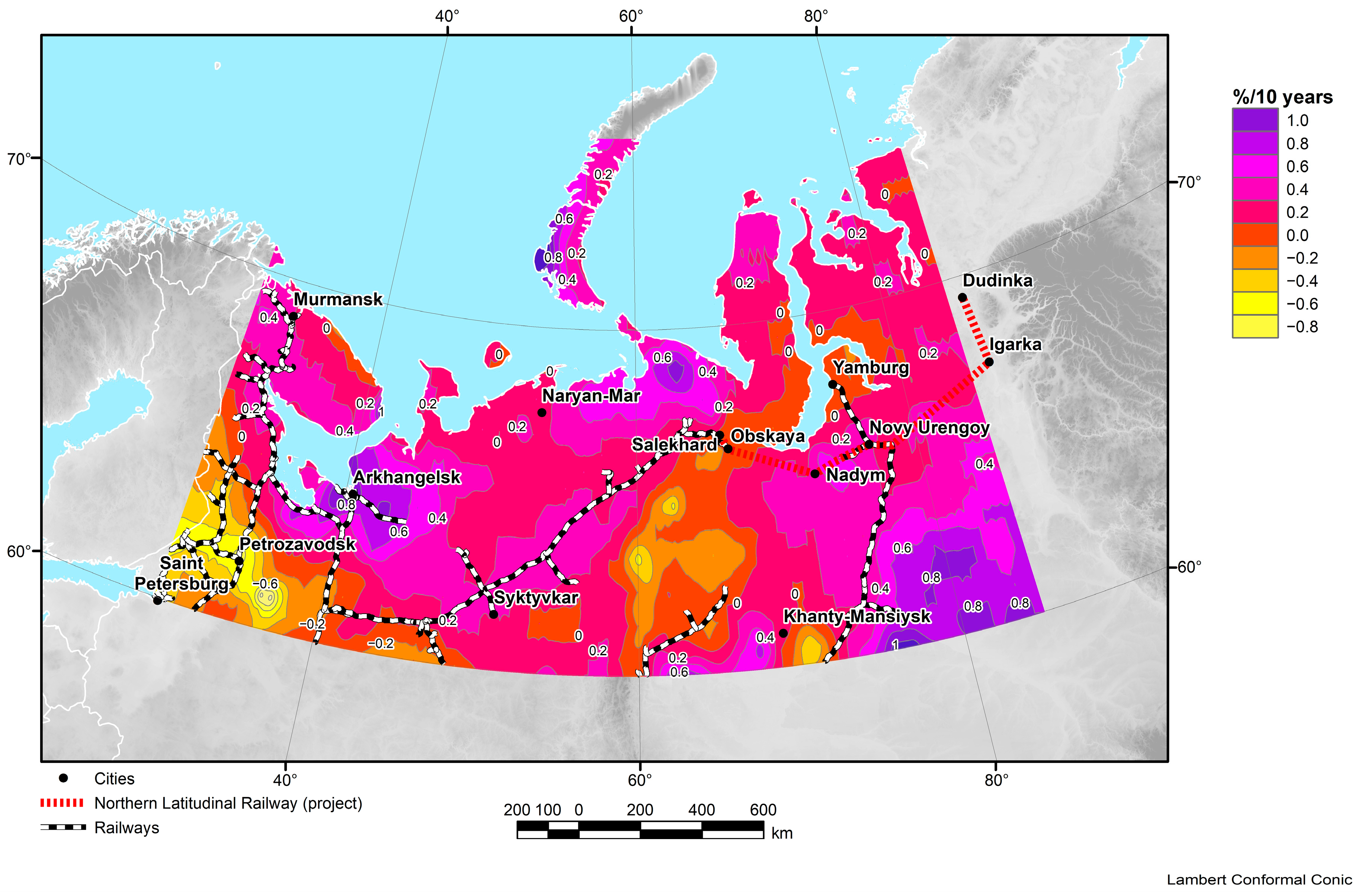
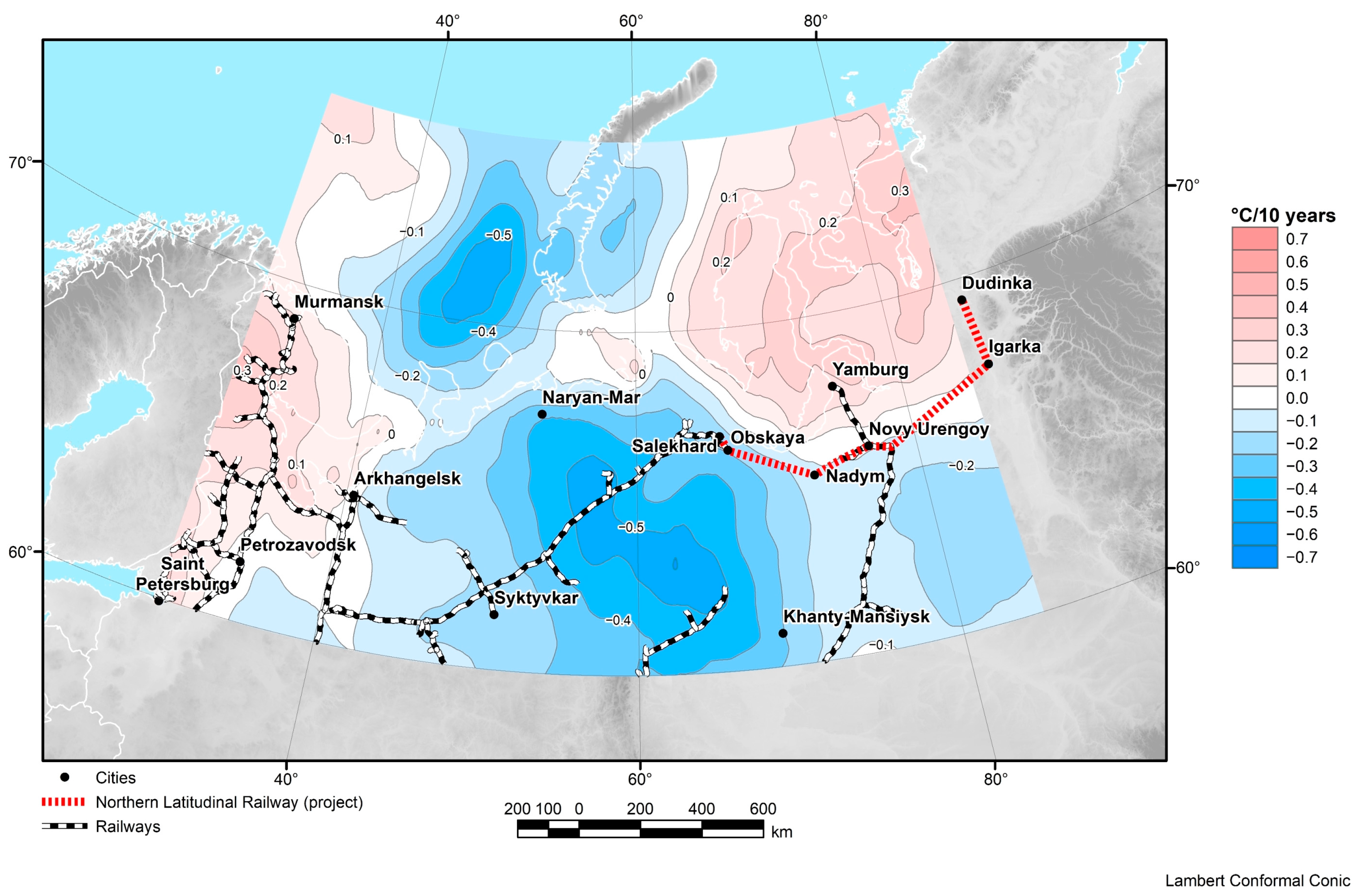
Not only the rate, but also the direction of air temperature change varied radically from 1980 to 2021. If in 1980–1999, almost the whole studied area was cooling at a rate from 0 °C to 0.5 °C per 10 years. In Figure 23 (except for the Kola Peninsula and Karelia, where warming was 0.2 °C per 10 years), in 2000–2021, warming was observed everywhere from 0.1 °C to 0.5 °C per 10 years and the farther northwards, and it was faster on average in Figure 24.
Atmospheric precipitation in the studied area was on average 1.8–2.4 in/day, and the average values for 1980–2021 are distributed regularly over the territory, except for the Ob Bay area, where precipitation is less in Figure 17. Difference in mean precipitation between 1980–1999 and 2000–2021 shows that precipitation has increased by 0.06–0.12 in/day on railway sections to Murmansk, by 0.10–0.16 in/day to Arkhangelsk and Salekhard and remained virtually unchanged along the section to Yamburg in 
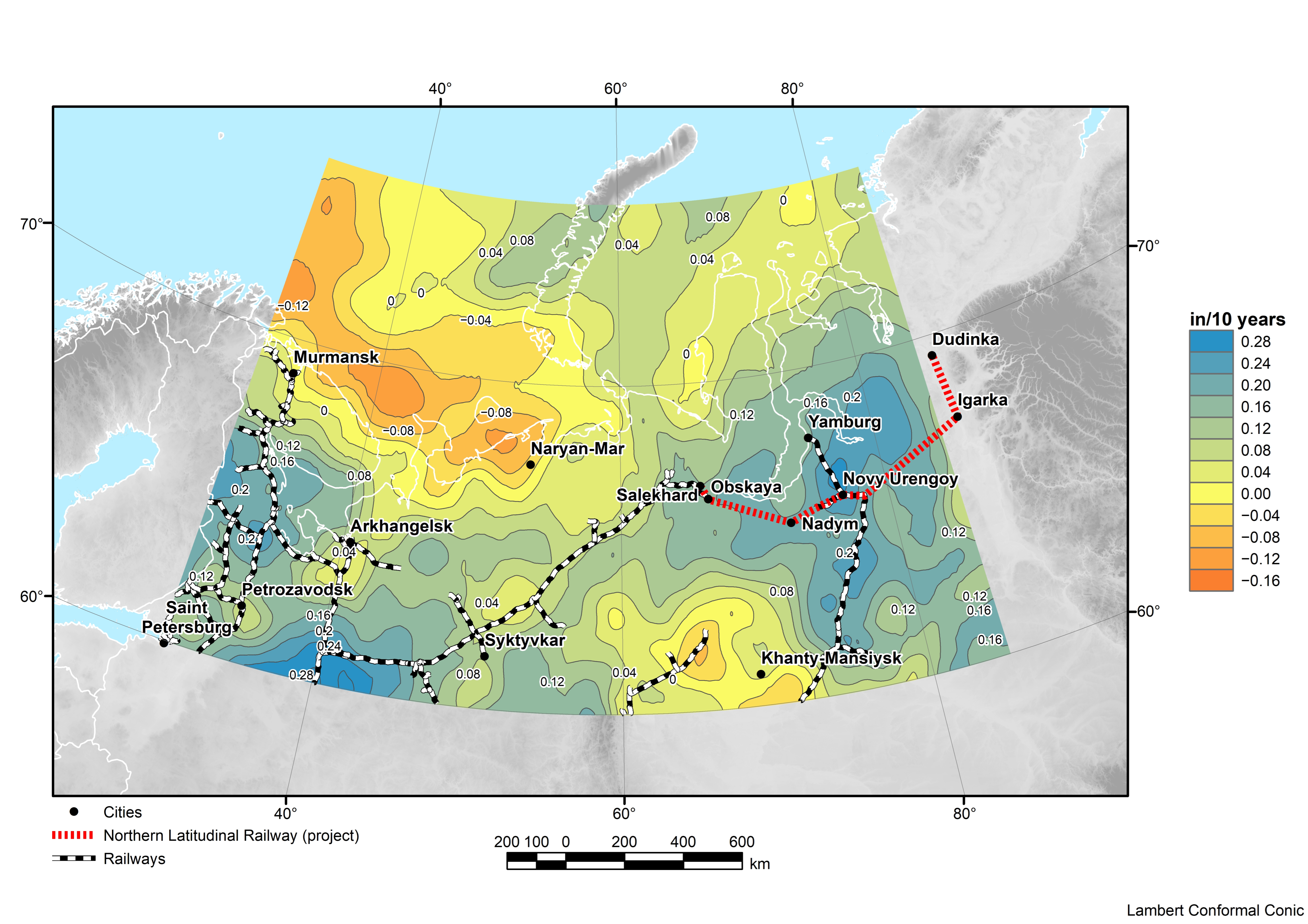
Figure 25. These changes are only 5% of the average values, so in the mean this increase is insignificant. However, in areas where average air temperatures have crossed 0 °C, this may indicate predominantly rain rather than snow, but this requires a joint analysis of air temperature and precipitation changes for individual months. Intra-annual variability shows that the greatest amount of precipitation in the studied area occurs from June to August. The most significant changes between the periods 1980–1999 and 2000–2021 occurred in March in the central part of the studied territory, where precipitation increased by 0.2–0.5 in/day. In May, near Arkhangelsk the increase was 0.5 in/day; in June, along the railway to Salekhard the increase was 0.5–1.0 in/day; in August, at some sections of the Murmansk and Arkhangelsk railways, as well as the railway to Yamburg, the increase was 0.6 in/day; in September, at some sections of the Murmansk and Arkhangelsk railways, as well as along the railway between Syktyvkar and Salekhard, the increase was 0.4–0.8 in/day. These changes in some months and in some areas are significant, increasing from 25 to 50% of the average values. In addition, the highest growth rate of precipitation was observed exactly in the last 20 years, when it reached 0.15–0.2 in/day per 10 years, i.e., approximately 10% for 10 years along almost all railway sections in Figure 26.
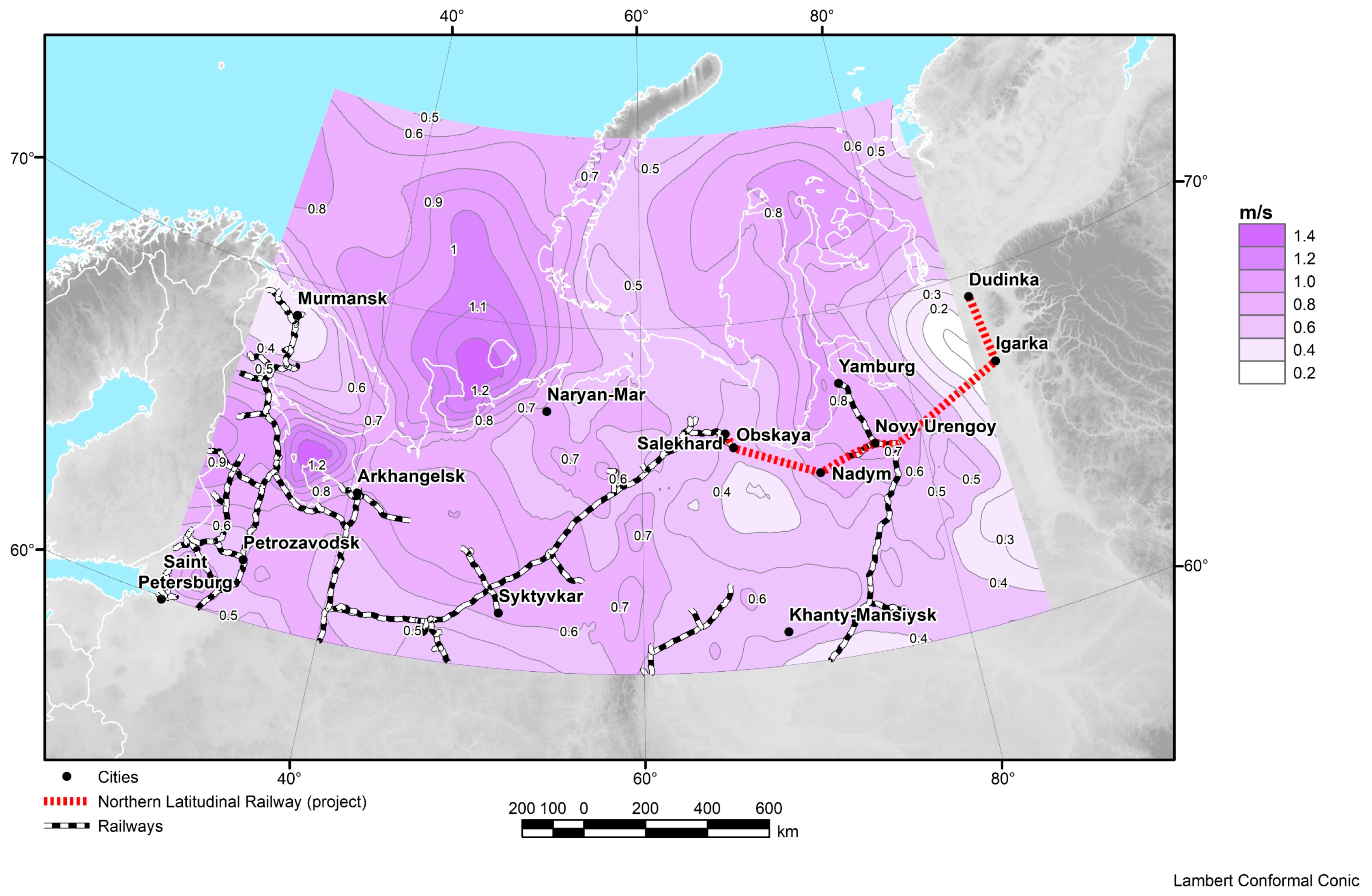
Average wind speed in the region ranges from 1.0 to 1.5 m/s for 1980–2021. This is the southwestern wind within all the studied area. Between the 1980–1999 and 2000–2021 periods, the wind speed has increased in some areas by 0.10–0.15 m/s, which is 10% of the average values. There is a significant seasonal variability in wind speed, which changes on average from 1 m/s in summer (June–August) to 2–3 m/s in winter (December–February). In some months and in some areas, the observed changes are even more significant. For example, between the periods 1980–1999 and 2000–2021, in March, the wind speed increased by 0.5 m/s along the railway to Yamburg. In April, the same wind speed increase was observed on the same railway to Salekhard and on the Murmansk railway. In June, the same wind speed increase was observed in the vast area around Syktyvkar. In July, the wind speed increased by 0.5–1.0 m/s near Salekhard and Yamburg. In August, the wind speed increased by 0.5 m/s in Karelia, at the railway sections to Salekhard and Yamburg, and in September by 0.5 m/s everywhere in 
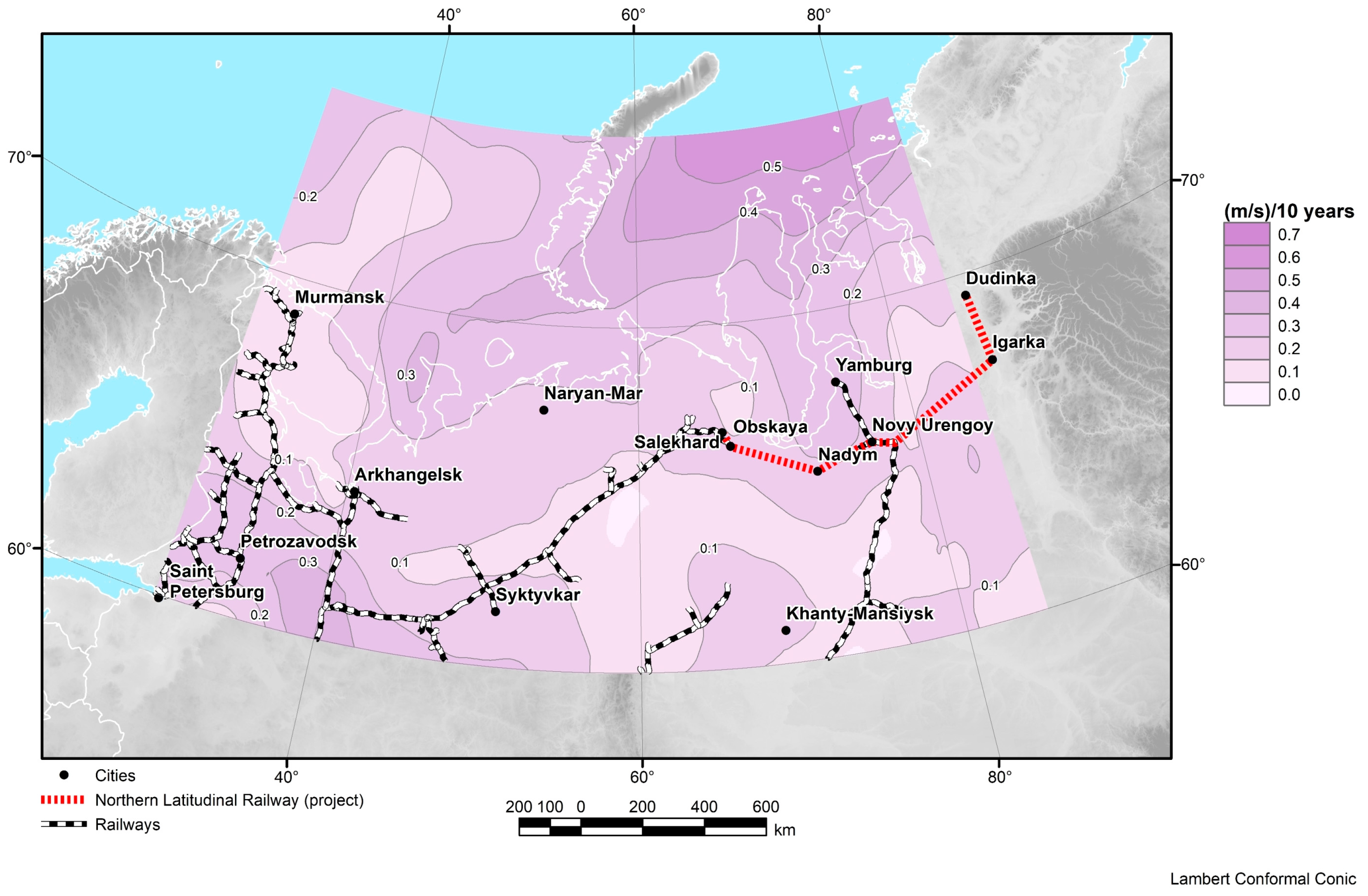
Figure 27. In the central part of the studied area, the wind speed growth rate in the last 20 years reached 0.1 m/s per 10 years, which is about 10% per decade in Figure 28.
In the last two decades, the average snow cover thickness in the studied area was 20–35 cm in Figure 29. The observed climate warming led to a decrease in snow cover thickness from 1980–1999 to 2000–2021 by 2–4 cm in the western and eastern parts of this territory, i.e., by approximately 10% in Figure 21. The highest snow cover thickness is observed in March, when it reaches 50–80 cm in different regions, and from 70 to 100 cm along the railway from Syktyvkar to Salekhard in Figure 30. From June to September, the snow cover is absent. The rate of snow cover reduction can reach 2.5–3.5 cm per 10 years in the northern part of this region, both on the Kola Peninsula and in the area of the Gulf of Ob.
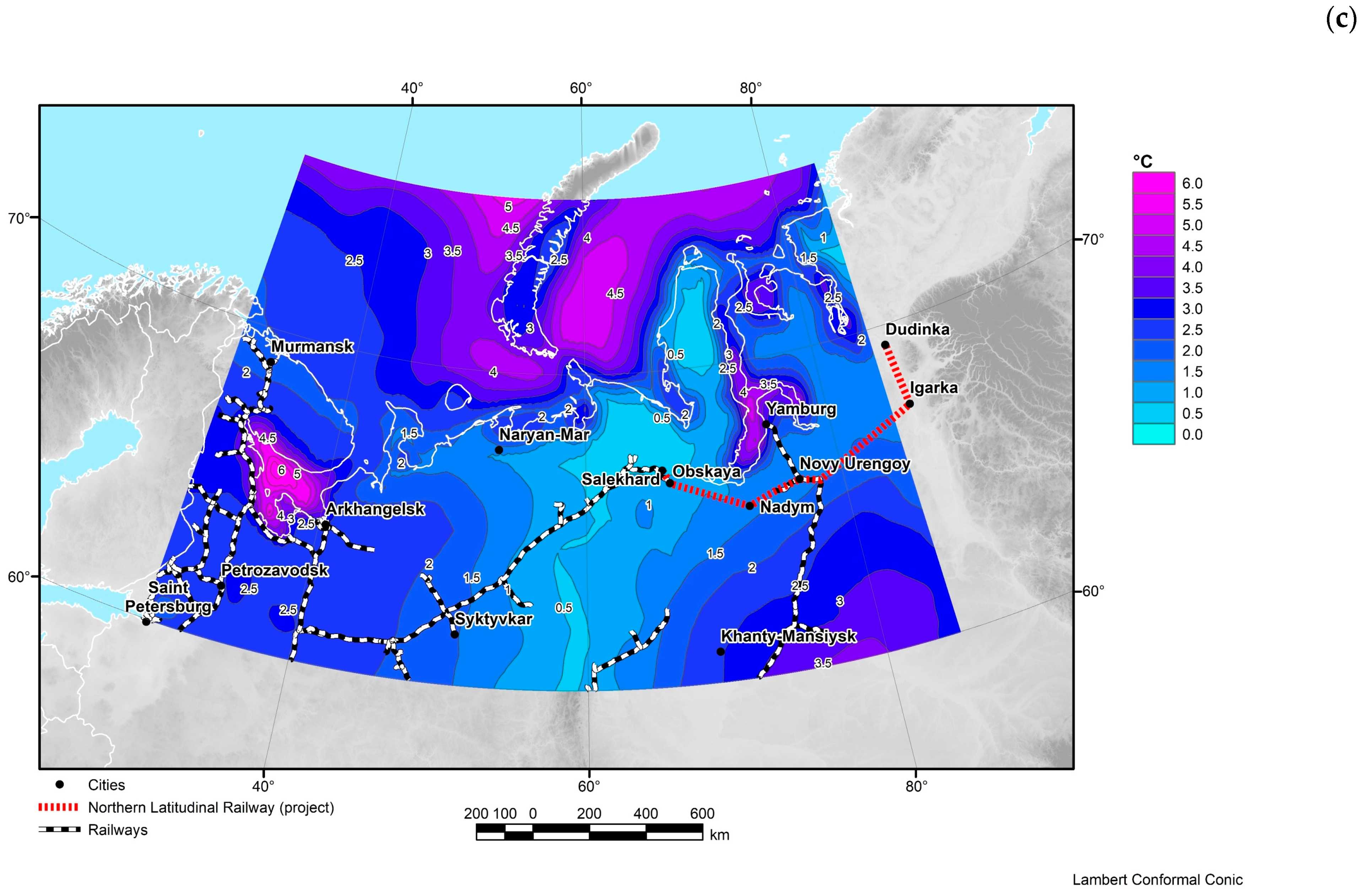
Soil temperature increased significantly along with the climate warming [62]. Average changes in temperature of the upper 10 m of soil between the periods 1980–1999 and 2000–2021 varied from 0.2 °C to 0.8 °C. This warming affected the area westwards from the Ural Mountains; the area eastwards remained virtually unaffected in Figure 31. The spatial distribution of soil temperature in the last two decades is shown in Figure 17. Notably, in both average values and in values for individual months, negative values of soil temperature in the MERRA-2 database are observed only on the Novaya Zemlya Archipelago, Yamal Peninsula, and northwards from 68°N in the territory east of the Gulf of Ob. This distribution contradicts the known maps of the permafrost boundary position in northern Russia and Siberia [3,6], so this issue requires special consideration. The average rate of soil temperature increased in 2000–2021 and reached from 0.2 °C to 0.8 °C per 10 years in the central part of the studied area whereas in the far northern regions it reached from 1.2 °C to 1.6 °C per 10 years in Figure 32.
In this section, we discussed only those specific features of the regional climate change in terms of seasonal and interannual variability of seven meteo-parameters which, from our point of view, are the most significant for consideration by railway operators. For the first time, such an analysis was completed specially for the western part of the Russian Arctic where a dense railway network exists and there are plans for its development in the near future. The obtained information is unique, because we concisely discussed every parameter and presented the main key peculiarities of the regional climate change for different sections of the railway network where the greatest changes were observed. To our knowledge supported by the opinion of the experts from Research and Design Institute of Informatization, Automation and Communications in Railway Transport, which belongs to the Russian railways, this is the first digital atlas of climate change impact on operability and infrastructure of the Russian railways in the Russian Federation.
For instance, the “Third assessment report on climate change and its consequences on the territory of the Russian Federation” issued in October 2022 by the Russian Hydrometeorological Service [63], which is the most comprehensive recent analysis of climate change on the territory and aquatoria of the Russian Federation, contains only very general and very limited information about the impact on the Russian railways in the volume of 3.5 pages from 678 pages in total. Moreover, this concerns both automobile and railway transport.
There is a long list of publications and reviews devoted to climate change impact on railway transport operability and infrastructure in different countries, but all of them dis-cuss general negative issues from heat or cold waves, frosts, permafrost thawing, heavy rains, storms and high winds, extreme sea level and waves, riverine and coastal storm flooding, and show different case studies of this impact [2,64,65,66,67,68,69,70,71,72,73,74,75,76]. However, we could not find a detailed atlas such as this one with a comprehensive set of different maps and parameters which display the ongoing regional climate change and its impact on railway networks in other parts of the world.

5. Conclusions

The atlas depicting climatic changes of basic hydrometeorological parameters in the western part of the Russian Arctic over 1950–2021 is the first experience of building a specialized climatic cartographic product for the needs of the Russian railways [77]. It contains 459 maps of mean seasonal and decadal characteristics of surface air temperature (69 maps), total precipitation (69 maps), wind speed at ground surface (69 maps), soil temperature (63 maps), soil moisture (63 maps), air humidity (63 maps), and snow cover thickness (63 maps), along with their mean rates of change (linear trends). This article details the initial data and GIS-based methodology used for compiling the atlas; and provides its main features and examples of certain map types. In addition, it discusses the most intriguing results that come from the interannual variability of the studied parameters, which are crucial for the railway operation in the northwestern part of the Russian Arctic.
We show that the climate warming in the studied area is very irregular within a year (by months), spatially, and even along each section of the railway (from 0.5 °C to 2.6 °C between 1980–1999 and 2000–2021). The rate of air temperature increase is maximal exactly in the last 20 years and reaches 0.5 °C per 10 years. The observed climate warming led to a 2–4 cm reduction in snow cover thickness from 1980–1999 to 2000–2021 in the western and eastern parts of the studied area, i.e., by approximately 10%. As the climate is becoming warmer, soil temperatures increase significantly. Average temperature change in the upper 10 m of soil between the 1980–1999 and 2000–2021 periods varies from 0.2 °C to 0.8 °C. Between 1980–1999 and 2000–2021, there is a significant increase in precipitation, which in some months and in some areas ranges from 25% to 50% of average values. The highest rate of precipitation growth is observed precisely within the last 20 years, when it reaches 10% per 10 years along almost all railway sections.
The performed analysis has revealed significant spatial and temporal heterogeneity of the considered parameters variability. These results suggest that a thorough study of the climatic parameters along each railway section separately is needed. This will make it possible to clarify the observed changes and improve the forecast for individual railway sections. The future research in this direction will result in: (1) creation of specialized diagrams (Hovmöller diagram) of spatial and temporal variability of selected hydrometeorological parameters along the main railway sections in the northwestern part of the Russian Arctic; (2) creation of maps and diagrams of spatial and temporal variability of extreme weather phenomena in the form of observed anomalies, occurrence frequency and duration; (3) creation of forecast maps of spatial and temporal variability of basic hydrometeorological parameters up to the end of the 21st century for the existing and planned railway infrastructure.
Particular strengths of this study concern a choice of the meteo-parameters, specification of the maps, visual representations of the maps (color scales, isolines, railway lines, rivers, coastlines, geographical projection, etc.), original algorithms of geospatial data processing and their representation in the in GIS environment, and our own recommendations derived from the research on how to improve future generations of the atlas. This is why we describe in detail technical aspects of the atlas construction that can be used by our followers to avoid mistakes and save time in building atlases for other similar regions in the world.
This is the first experience in building a specialized climatic cartographic product for the needs of the Russian railways, and to our knowledge the first atlas such as that in the world. The atlas expansion and improvement will be continued in the framework of the Russian Science Foundation Project No. 21-77-30010 (2021–2024) “System analysis of geophysical process dynamics in the Russian Arctic and their impact on the development and operation of the railway infrastructure” in close collaboration with experts from the Russian railways.
We hope that the detailed analysis of the atlas maps prepared for the Russian rail-ways, along with its future expansion, will contribute to sustainable development and adaptation of the railway infrastructure to climate change in the northwestern part of the Russian Arctic. In the future, the amassed experience may be transferred to other regions of the Russian Federation, as well as similar regions in Canada, Sweden, and Highland China that are also subject to significant climate change [72,76].

Author Contributions

Conceptualization, A.D.G., I.N.R. and A.A.S.; methodology, map validation, writing—climatic aspect, A.G.K.; software compilation and climatic data processing, I.V.S.; map design, figure preparation, writing, S.A.G., A.B.P. and G.A.G.; writing—transport aspect, N.V.S. and I.A.D.; writing—economical aspect, E.A.K.; supervision, review and editing, R.I.K. All authors have read and agreed to the published version of the manuscript.

Funding

The analysis and interpretation of climatic data and atlas maps presented in this paper were funded by the Russian Science Foundation (Project No. 21-77-30010) “System analysis of geophysical process dynamics in the Russian Arctic and their impact on the development and operation of the railway infrastructure”.

Institutional Review Board Statement

Not applicable.

Informed Consent Statement

Not applicable.

Data Availability Statement

Not applicable.

Acknowledgments

The atlas of hydrometeorological parameters was compiled in the framework of the project with the Research and Design Institute of Informatization, Automation and Communications in Railway Transport. The authors wish to thank the scientific teams of the responsible agencies and institutions for the provided data.

Conflicts of Interest

The authors declare no conflict of interest.

References

  1. Katzov, V.M.; Akenteva, E.M.; Anisimov, O.A.; Gruza, G.V.; Zaitsev, A.E.; Frolov, I.E.; Sirotenko, A.D.; Kattsov, V.M.; Karol, I.E.; Terziev, F.S.; et al. Third Assessment Report on Climate Change and Its Consequences on the Territory of the Russian Federation. General Summary; Science-Intensive Technologies (Naukoyemkie Technologii): St. Petersburg, Russia, 2022; pp. 22–30. [Google Scholar]
  2. Masson-Delmotte, V.; Zhai, P.; Pirani, A.; Connors, S.L.; Péan, C.; Berger, S.; Caud, N.; Chen, Y.; Goldfarb, L.; Gomis, M.I.; et al. (Eds.) Climate Change 2021: The Physical Science Basis. Contribution of Working Group I to the Sixth Assessment Report of the Intergovernmental Panel on Climate Change; Cambridge University Press: Cambridge, UK; New York, NY, USA, 2021; 2391p. [Google Scholar]
  3. Kostianaia, E.A.; Kostianoy, A.G.; Scheglov, M.A.; Karelov, A.I.; Vasileisky, A.S. Impact of regional climate change on the infrastructure and operability of railway transport. Transp. Telecommun. 2021, 22, 183–195. [Google Scholar] [CrossRef]
  4. Yakubovich, A.N.; Yakubovich, I.A. Forecasting the impact of climatic changes on the functionality of the transport infrastructure of the permafrost zone in Russia. Intellect. Innovation. Invest. 2019, 1, 104–110. [Google Scholar] [CrossRef]
  5. Serykh, I.V.; Kostianoy, A.G.; Lebedev, S.A.; Kostianaia, E.A. On the transition of temperature regime of the White Sea Region to a new phase state. Fund. App. Hydrophys. 2022, 15, 98–111. [Google Scholar]
  6. Osipov, V.I.; Rumyantseva, N.A.; Eremina, O.N. Living with risk of natural disasters. Russ. J. Earth Sci. 2019, 19, 1–10. [Google Scholar] [CrossRef] [Green Version]
  7. Romanenko, F.A.; Shilovtseva, O.A. Geomorphological processes in the mountains of the Kola Peninsula and climate change. MSU Vestnik Ser. 5 Geog. 2016, 6, 78–86. (In Russian) [Google Scholar]
  8. World Experience in the Construction, Maintenance and Repair of Railway Infrastructure Facilities in Permafrost Conditions; Center for Scientific and Technical Information and Libraries: Moscow, Russia, 2017; 126p. (In Russian)
  9. Rosstat. Socio-Economic Situation of the North-Western Federal District. Available online: https://rosstat.gov.ru/storage/mediabank/Sev-Zap-fo_1k-2022.pdf (accessed on 1 November 2022).
  10. Rosstat. Socio-Economic Situation of the Ural Federal District. Available online: https://rosstat.gov.ru/storage/mediabank/Ural-fo_1k-2022.pdf (accessed on 1 November 2022).
  11. Northern Latitudinal Railway. Available online: http://uralfo.gov.ru/projects/sshh/ (accessed on 1 November 2022).
  12. Northern Latitudinal Railway. Available online: http://www.cupp.ru/karta-proekta/ (accessed on 1 November 2022).
  13. Verezemskaya, P.; Selivanova, Y.; Tilinina, N.; Markina, M.; Krinitskiy, M.; Sharmar, V.; Razorenova, O. Projected changes in the near-surface atmosphere over the Barents Sea based on CMIP5 scenarios. Russ. J. Earth. Sci. 2022, 22. [Google Scholar] [CrossRef]
  14. Gelaro, R.; McCarty, W.; Suárez, M.J.; Todling, R.; Molod, A.; Takacs, L.; Randles, C.A.; Darmenov, A.; Bosilovich, M.G.; Reichle, R.; et al. The Modern-Era Retrospective Analysis for Research and Applications, Version 2 (MERRA-2). J. Clim. 2017, 30, 5419–5454. [Google Scholar] [CrossRef]
  15. McCarty, W.; Coy, L.; Gelaro, R.; Huang, A.; Merkova, D.; Smith, E.B.; Sienkiewicz, M.; Wargan, K. MERRA-2 input observations: Summary and initial assessment. Tech. Rep. Ser. Glob. Model. Data Assim. 2016, 46, 61. [Google Scholar]
  16. Bosilovich, M.G. Regional Climate and Variability of NASA MERRA and Recent Reanalyses: U.S. Summertime Precipitation and Temperature. J. Appl. Meteorol. Climatol. 2013, 52, 1939–1951. [Google Scholar] [CrossRef]
  17. Tilinina, N.; Gulev, S.K.; Rudeva, I.; Koltermann, K.P. Comparing cyclone life cycle characteristics and their interannual variability in different reanalyses. J. Clim. 2013, 26, 6419–6438. [Google Scholar] [CrossRef] [Green Version]
  18. Bentamy, A.; Piollé, J.F.; Grouazel, A.; Danielson, R.; Gulev, S.; Paul, F.; Azelmat, H.; Mathieu, P.P.; von Schuckmann, K.; Sathyendranah, S.; et al. Review and assessment of latent and sensible heat flux accuracy over the global oceans. Remote Sens. Environ. 2017, 201, 196–218. [Google Scholar] [CrossRef] [Green Version]
  19. Luo, B.; Minnett, P.; Szczodrak, M.; Nalli, M.; Morris, V. Accuracy assessment of MERRA-2 and ERA-Interim sea-surface temperature, air temperature and humidity profiles over the Atlantic Ocean using AEROSE measurements. J. Clim. 2020, 33, 6889–6909. [Google Scholar] [CrossRef]
  20. Sharmar, V.; Markina, M. Evaluation of interdecadal trends in sea ice, surface winds and ocean waves in the Arctic in 1980–2019. Russ. J. Earth. Sci. 2021, 21, 3. [Google Scholar] [CrossRef]
  21. Schubert, S.D.; Chang, Y.; DeAngelis, A.M.; Koster, R.D.; Lim, Y.; Wang, H. Exceptional Warmth in the Northern Hemisphere during January–March of 2020: The Roles of Unforced and Forced Modes of Atmospheric Variability. J. Clim. 2022, 35, 2565–2584. [Google Scholar] [CrossRef]
  22. Kalnay, E.; Kanamitsu, M.; Kistler, R.; Collins, W.; Deaven, D.; Gandin, L.; Joseph, D. The NCEP/NCAR 40-year reanalysis project. Bull. Am. Meteorol. Soc. 1996, 77, 437–471. [Google Scholar] [CrossRef]
  23. The International Institute for Applied Systems Analysis (IIASA), Russian Academy of Sciences (RAS). 2002. Land Resources of Russia. Available online: http://www.iiasa.ac.at/Research/FOR/russia_cd/download.htm (accessed on 3 November 2022).
  24. Si, Z.; Li, S.; Huang, L.; Chen, Y. Visualization programming for batch processing of contour maps based on VB and Surfer software. Adv. Eng. Softw. 2010, 41, 962–965. [Google Scholar] [CrossRef]
  25. Golden Software Surfer. Available online: https://www.goldensoftware.com/products/surfer (accessed on 1 November 2022).
  26. ESRI ArcMap. Available online: https://www.esri.com/en-us/arcgis/products/arcgisdesktop/resources (accessed on 3 November 2022).
  27. Bartuś, T. Raster images generalization in the context of research on the structure of landscape and geodiversity. Geol. Geophys. Environ. 2014, 40, 271–284. [Google Scholar] [CrossRef] [Green Version]
  28. Watson, C.; Richardson, J.; Wood, B.; Jackson, C.; Hughes, A. Improving geological and process model integration through TIN to 3D grid conversion. Comp. Geosci. 2015, 82, 45–54. [Google Scholar] [CrossRef] [Green Version]
  29. Theoretical Fundaments in Geoinformation Systems (GIS). Available online: https://desktop.arcgis.com/ru/arcmap/latest/extensions/3d-analyst/fundamentals-of-3dsurfaces.htm (accessed on 30 October 2022).
  30. Soloviev, A.A.; Krasnoperov, R.I.; Nikolov, B.P.; Zharkikh, J.I.; Agayan, S.M. Web-oriented software system for analysis of spatial geophysical data using geoinformatics methods. Izv. Atm. Ocean. Phys. 2018, 54, 1312–1319. [Google Scholar] [CrossRef]
  31. Islam, M.S. Assessing the dynamics of land cover and shoreline changes of Nijhum Dwip (Island) of Bangladesh using remote sensing and GIS techniques. Reg. Stud. Mar. Sci. 2021, 41, 101578. [Google Scholar] [CrossRef]
  32. Built-In Processing Tools Technical Support, ArcMap. Available online: https://support.esri.com/en/technical-article/000013000 (accessed on 2 November 2022).
  33. A Source Code of Author’s Tool to Clip Unnecessary Values. The Tool for ArcGIS. Available online: https://github.com/GAGvozdik/Group_raster_clip (accessed on 1 November 2022).
  34. Yang, C.S.; Kao, S.P.; Lee, F.B.; Hung, P.S. Twelve different interpolation methods: A case study of Surfer 8.0. In Proceedings of the XXth ISPRS Congress, Istanbul, Turkey, 12–23 July 2004. [Google Scholar]
  35. Kriging. Available online: https://surferhelp.goldensoftware.com/griddata/idd_grid_data_kriging.htm (accessed on 27 March 2023).
  36. Williams, R.T. Lambert and Mercator map projections in geology and geophysics. Comp. Geosci. 1995, 21, 353–364. [Google Scholar] [CrossRef]
  37. Spatial Reference System Information for ESPG. Available online: https://products.aspose.app/gis/epsg/code-102027 (accessed on 2 November 2022).
  38. Boyarshinov, G.; Popov, A.; Odintsova, A.; Gvozdik, S.; Rybkina, A.; Korolkova, A. Application of Geoportal’s Web-Technologies in GIS, Case Study: Interactive Geology Atlas. Russ. J. Earth. Sci. 2022, 22, 3002. [Google Scholar] [CrossRef]
  39. About Analyzing Images and Raster Data. Available online: https://desktop.arcgis.com/ru/arcmap/latest/manage-data/raster-and-images/about-analyzingimagery-raster-data.htm (accessed on 4 November 2022).
  40. Habel, M.; Obodovskyi, O.; Szatten, D.; Babinski, Z.; Rozlach, Z.; Pochaievets, O. Using the raster calculator tool to appraise riverbed elevation changes nearby hydrotechnical objects on alluvial rivers. Eur. Assoc. Geosci. Eng. 2019, 2019, 1–5. [Google Scholar] [CrossRef]
  41. Description of Raster Calculator Utilization. Available online: https://desktop.arcgis.com/ru/arcmap/10.5/tools/spatial-analyst-toolbox/raster-calculator.htm (accessed on 1 November 2022).
  42. Serykh, I.V.; Tolstikov, A.V. Climate change in the western part of the Russian Arctic in 1980–2021. Part 1. Air temperature, precipitation, wind. Arct. Antarct. Res. 2022, 68, 258–277. [Google Scholar] [CrossRef]
  43. Serykh, I.V.; Tolstikov, A.V. Climate change in the western part of the Russian Arctic in 1980–2021. Part 2. Soil temperature, snow, humidity. Arct. Antarct. Res. 2022, 68, 352–369. [Google Scholar] [CrossRef]
  44. Han, Y.; Revercomb, H.; Cromp, M.; Gu, D.; Johnson, D.; Mooney, D.; Scott, D.; Strow, L.; Bingham, G.; Borg, L.; et al. Suomi NPP CrIS measurements, sensor data record algorithm, calibration and validation activities, and record data quality. J. Geophys. Res. Atmos. 2013, 118, 12734–12748. [Google Scholar] [CrossRef]
  45. Kim, E.; Lyu, C.H.J.; Anderson, K.; Leslie, R.V.; Blackwell, W.J. S-NPP ATMS instrument prelaunch and on-orbit performance evaluation. J. Geophys. Res. 2014, 119, 5653–5670. [Google Scholar] [CrossRef] [Green Version]
  46. Chen, M.; Xie, P.; Janowiak, J.E.; Arkin, P.A. Global Land Precipitation: A 50-yr Monthly Analysis Based on Gauge Observations. J. Hydrometeorol. 2002, 3, 249–266. [Google Scholar] [CrossRef]
  47. Reichle, R.H.; Koster, R.D.; De Lannoy, G.J.; Forman, B.A.; Liu, Q.; Mahanama, S.P.P.; Toure, A. Assessment and enhancement of MERRA land surface hydrology estimates. J. Clim. 2011, 24, 6322–6338. [Google Scholar] [CrossRef] [Green Version]
  48. Bosilovich, M.G.; Lucchesi, R.; Suarez, M. MERRA-2: File Specification; GMAO Office Note No. 9 (Version 1.1); NASA: Greenbelt, MD, USA, 2016; pp. 1–75.
  49. Poli, P.; Hersbach, H.; Tan, D.; Dee, D.; Thépaut, J.; Simmons, A.; Peubey, C.; Laloyaux, P.; Komori, T.; Berrisford, P.; et al. The Data Assimilation System and Initial Performance Evaluation of the Ecmwf Pilot Reanalysis of the 20th-Century Assimilating Surface Observations Only (ERA-20C); European Centre for Medium-Range Weather Forecasts: Shinfield Park, UK, 2013; pp. 1–59. [Google Scholar]
  50. Ma, H.; Zeng, J.; Zhang, X.; Fu, P.; Zheng, D.; Wigneron, J.; Chen, N.; Niyogi, D. Evaluation of six satellite- and model-based surface soil temperature datasets using global ground-based observations. Remote Sens. Environ. 2021, 264, 112605. [Google Scholar] [CrossRef]
  51. Reichle, R.H.; Draper, C.S.; Liu, Q.; Girotto, M.; Mahanama, P.P.; Koster, R.D.; De Lannoy, G.J. Assessment of MERRA-2 Land Surface Hydrology Estimates. J. Clim. 2017, 30, 2937–2960. [Google Scholar] [CrossRef] [Green Version]
  52. Dee, D.P.; da Silva, A.M. The choice of variable for atmospheric moisture analysis. Mon. Weather. Rev. 2003, 131, 155–171. [Google Scholar] [CrossRef]
  53. Holm, E.V. Revision of the ECMWF humidity analysis: Construction of a Gaussian control variable. In Proceedings of the ECMWF/GEWEX Workshop on Humidity Analysis, Reading, UK, 8–11 July 2003. [Google Scholar]
  54. Tao, J.; Koster, R.D.; Reichle, R.H.; Forman, B.A.; Xue, Y.; Chen, R.H.; Moghaddam, M. Permafrost Variability over the Northern Hemisphere Based on the MERRA2 Reanalysis. Cryosphere 2019, 13, 2087–2110. [Google Scholar] [CrossRef] [Green Version]
  55. Toure, A.M.; Reichle, R.H.; Forman, B.A.; Getirana, A.; De Lannoy, G.J. Assimilation of MODIS Snow Cover Fraction Observations into the NASA Catchment Land Surface Model. Remote Sens. 2018, 10, 316. [Google Scholar] [CrossRef] [Green Version]
  56. Information Resources: Basic Geographical Backgrounds. Available online: https://vsegei.ru/ru/info/topo/ (accessed on 31 October 2022).
  57. Gvishiani, A.D.; Kaftan, V.I.; Krasnoperov, R.I.; Tatarinov, V.N.; Vavilin, E.V. Geoinformatics and systems analysis in geophysics and geodynamics. Izv. Phys. Sol. Earth 2019, 55, 33–49. [Google Scholar] [CrossRef]
  58. Lemenkova, P. GEBCO Gridded Bathymetric Datasets for Mapping Japan Trench Geomorphology by Means of GMT Scripting Toolset. Geod. Cartogr. 2020, 46, 98–112. [Google Scholar] [CrossRef]
  59. General Bathymetric Chart of the Ocean, GEBCO. Available online: https://www.gebco.net/data_and_products/gridded_bathymetry_data/grid_production/ (accessed on 1 November 2022).
  60. Russian-language Database of Names with Specific Addresses Based on VMap0 Data. Available online: https://gis-lab.info/qa/vmap0-settl-rus.html (accessed on 2 October 2022).
  61. Petrunin, A.G.; Soloviev, A.A.; Sidorov, R.V.; Gvishiani, A.D. Inverse-forward method for heat flow estimation: Case study for the Arctic region. Russ. J. Earth Sci. 2022, 21, ES6004. [Google Scholar] [CrossRef]
  62. Al-shateri, H.A.A. Estimation of land surface temperature and distribution across Land use/land cover in response to coal mining activity in V. D. Yelevsky coal mine area–Russia. Russ. J. Earth Sci. 2022, 22, 5. [Google Scholar] [CrossRef]
  63. Katzov, V.M. (Ed.) . The Third Assessment Report on Climate Changes and Their Consequences on the Territory of the Russian Federation; Science-Intensive technologies (Naukoyemkie Technologii): St. Petersburg, Russia, 2022; 678p. [Google Scholar]
  64. Baker, C.J.; Chapman, L.; Quinn, A.; Dobney, K. Climate Change and the Railway Industry: A Review. [Online]. 2009. Available online: http://journals.sagepub.com/doi/pdf/10.1243/09544062JMES1558 (accessed on 6 April 2023).
  65. Nemry, F.; Demirel, H. Impacts of Climate Change on Transport: A Focus on Road and Rail Transport Infrastructures. [Online]. 2012. Available online: http://ftp.jrc.es/EURdoc/JRC72217.pdf (accessed on 6 April 2023).
  66. Oslakovic, I.S.; ter Maat, H.W.; Hartmann, A.; Dewulf, G. Risk Assessment of Climate Change Impacts on Railway Infrastructure. [Online]. 2013. Available online: https://core.ac.uk/download/pdf/29215286.pdf (accessed on 6 April 2023).
  67. Rail Safety and Standards Board. Tomorrow’s Railway and Climate Change Adaptation: Executive Report. [Online]. 2016. Available online: www.rssb.co.uk (accessed on 6 April 2023).
  68. Palco, K.; Lemmen, D.S. (Eds.) Climate Risks and Adaptation Practices for the Canadian Transportation Sector; Government of Canada: Ottawa, ON, Canada, 2017; [Online]; Available online: http://www.nrcan.gc.ca/environment/impacts-adaptation10761 (accessed on 6 April 2023).
  69. Bubeck, P.; Dillenardt, L.; Alfieri, L.; Feyen, L.; Thieken, A.H.; Kellermann, P. Global warming to increase flood risk on European railways. Clim. Change 2019, 155, 19–36. [Google Scholar] [CrossRef]
  70. Koks, E.E.; Rozenberg, J.; Zorn, C.; Tariverdi, M.; Vousdoukas, M.; Fraser, S.A.; Hall, J.W.; Hallegatte, S. A global multi-hazard risk analysis of road and railway infrastructure assets. Nat. Comm. 2019, 10, 2677. [Google Scholar] [CrossRef] [Green Version]
  71. Climate Change Impacts and Adaptation for Transport Networks and Nodes. Report of United Nations Economic Commission for Europe (ECE), 2020, 216p. [Online]. Available online: https://unece.org/sites/default/files/2021-01/ECE-TRANS-283e_web.pdf (accessed on 6 April 2023).
  72. Thaduri, A.; Garmabaki, A.; Kumar, U. Impact of climate change on railway operation and maintenance in Sweden: A State-of-the-art review. Maint. Reliab. Cond. Monit. 2021, 1, 52–70. [Google Scholar] [CrossRef]
  73. Garmabaki, A.H.S.; Thaduri, A.; Famurewa, S.; Kumar, U. Adapting Railway Maintenance to Climate Change. Sustainability 2021, 13, 13856. [Google Scholar] [CrossRef]
  74. Palin, E.J.; Stipanovic Oslakovic, I.; Gavin, K.; Quinn, A. Implications of climate change for railway infrastructure. Wiley Interdiscip. Rev. Clim. Chang. 2021, 12, e728. [Google Scholar] [CrossRef]
  75. Ochsner, M.; Palmqvist, C.W. Weather and Train Disruptions in Sweden 2011–2019. In Proceedings of the 18th International Conference on Railway Engineering Design & Operation, Valencia, Spain, 21–23 September 2022. [Google Scholar]
  76. Kostianaia, E.A.; Kostianoy, A.G. Railway transport adaptation strategies to climate change at high latitudes: A review of experience from Canada, Sweden and China. Transp. Telecommun. 2023, 24, 180–194. [Google Scholar] [CrossRef]
  77. Rozenberg, I.N.; Gvishiani, A.D.; Soloviev, A.A.; Voronin, V.A.; Pilipenko, V.A. Influence of space weather on the reliability of railway transport in the Arctic zone of Russia. Railw. Transp. (Zheleznodorozhny Transp.) 2021, 12, 20–26. (In Russian) [Google Scholar]
Figure 1. Studied area.
Applsci 13 05278 g001
Figure 2. MERRA-2 observation points laid over the studied area.
Applsci 13 05278 g002
Figure 3. The data processing scheme for the atlas map compilation. The employed software is indicated in brackets.
Applsci 13 05278 g003
Figure 4. The Clip tool operation principle.
Applsci 13 05278 g004
Figure 5. Geographical location of the studied area. Thickened lines show the border of the AZRF (northwards from 60°N), as well as the western and eastern borders of the studied area (30–85° E).
Applsci 13 05278 g005
Figure 6. Comparison of spatial data: (a) within data groups (information on the average change in air temperature between the periods 1980–1999 and 2000–2021, comparison between the months January and July); (b) between data groups (comparison of average air temperature and precipitation for the period 1980–2021 for January).
Applsci 13 05278 g006aApplsci 13 05278 g006b
Figure 7. Example of the map design. Average air temperature changes (°C) between the periods 1980–1999 and 2000–2021 for the winter season (December–February).
Applsci 13 05278 g007
Figure 8. Scheme of the climatic atlas compilation.
Applsci 13 05278 g008
Figure 9. The result of the raster calculator tool application. The data represents the average change in air temperature (°C) between 1980–1999 and 2000–2021: (a) data for January; (b) data for July; (c) the resulting amplitude map of the average temperature between the two months, January and July.
Applsci 13 05278 g009aApplsci 13 05278 g009b
Figure 10. Map of average air temperature (°C) at 42.2 m altitude for the period 1950–2021 according to MERRA-2 data.
Applsci 13 05278 g010
Figure 11. Average rate of change in mean monthly anomalies of the soil upper layer moisture content (% per 10 years) for the period 1980–2021.
Applsci 13 05278 g011
Figure 12. Average rate of change in mean monthly anomalies (relative to the annual rate) of air temperature at 42.2 m (°C per 10 years) according to NCEP/NCAR Reanalysis for the period 1980–2021.
Applsci 13 05278 g012
Figure 13. Mean values of air temperature (°C) at 2 m for January according to MERRA-2 data for the period 1980–2021.
Applsci 13 05278 g013
Figure 14. Average values of total precipitation per day (in) according to MERRA-2 for the period 1980–2021.
Applsci 13 05278 g014
Figure 15. Average wind speed (m/s) at 50 m for the period 1980–2021.
Applsci 13 05278 g015
Figure 16. Average values of wind speed (m/s) at 50 m for the period 2000–2021: (a) for winter season (December–February); (b) for summer season (June–August).
Applsci 13 05278 g016
Figure 17. Mean values of temperature (°C) of the upper 10 m of soil for the period 2000–2021.
Applsci 13 05278 g017
Figure 18. Average values of the soil upper layer moisture content (%) for the period 1980–2021.
Applsci 13 05278 g018
Figure 19. Average values of specific humidity (g/kg) of air for the period 1980–2021.
Applsci 13 05278 g019
Figure 20. Average values of snow cover thickness (m) for the period 1980–2021.
Applsci 13 05278 g020
Figure 21. Average changes in snow cover thickness (m) between the periods 1980–1999 and 2000–2021 (difference of average values between these periods) according to MERRA-2 data.
Applsci 13 05278 g021
Figure 22. Average air temperature change (°C) at 2 m altitude between the periods 1980–1999 and 2000–2021 (difference of average values between these periods) for December.
Applsci 13 05278 g022
Figure 23. Average rate of change (linear trend) of mean monthly anomalies (relative to the annual rate) of air temperature at 2 m altitude (°C per 10 years) for 1980–1999.
Applsci 13 05278 g023
Figure 24. Average rate of change (linear trend) of mean monthly anomalies (relative to the annual rate) of air temperature at 2 m altitude (°C per 10 years) for 2000–2021.
Applsci 13 05278 g024
Figure 25. Average changes (difference in average values) in total precipitation per day (in) between the periods 1980–1999 and 2000–2021.
Applsci 13 05278 g025
Figure 26. Average rate (linear trend) of change in mean monthly anomalies (relative to the annual rate) of total precipitation per day (in/day per 10 years) over 2000–2021.
Applsci 13 05278 g026
Figure 27. Average wind speed change (m/s) (difference of average values) at 50 m altitude between the periods 1980–1999 and 2000–2021 for September.
Applsci 13 05278 g027
Figure 28. Average rate (linear trend) of wind speed change at 50 m altitude (m/s per 10 years) for 2000–2021.
Applsci 13 05278 g028
Figure 29. Average values of snow cover thickness (m) for 2000–2021.
Applsci 13 05278 g029
Figure 30. Average values of snow cover thickness (m) for March over 2000–2021.
Applsci 13 05278 g030
Figure 31. Average change (difference of average values) in temperature (°C) of the upper 10 m of soil between the periods 1980–1999 and 2000–2021.
Applsci 13 05278 g031
Figure 32. Average rate (linear trend) of change in mean monthly anomalies (relative to annual variation) of the temperature (°C per 10 years) of the upper 10 m of soil for 2000–2021.
Applsci 13 05278 g032
Disclaimer/Publisher’s Note: The statements, opinions and data contained in all publications are solely those of the individual author(s) and contributor(s) and not of MDPI and/or the editor(s). MDPI and/or the editor(s) disclaim responsibility for any injury to people or property resulting from any ideas, methods, instructions or products referred to in the content.

