Article

Dense-HR-GAN: A High-Resolution GAN Model with Dense Connection for Image Dehazing in Icing Wind Tunnel Environment

1
School of Computer Science, Southwest Petroleum University, Chengdu 610500, China
2
Key Laboratory of Icing and Anti/De-Icing, China Aerodynamics Research and Development Center, Mianyang 621000, China
*
Authors to whom correspondence should be addressed.
These authors contributed equally to this work.
Appl. Sci. 2023, 13(8), 5171; https://doi.org/10.3390/app13085171
Submission received: 24 March 2023 / Revised: 13 April 2023 / Accepted: 17 April 2023 / Published: 21 April 2023
(This article belongs to the Special Issue Advances in Image and Video Processing: Techniques and Applications)

Abstract

:
To address the issue of blurred images generated during ice wind tunnel tests, we propose a high-resolution dense-connection GAN model, named Dense-HR-GAN. This issue is caused by attenuation due to scattering and absorption when light passes through cloud and fog droplets. Dense-HR-GAN is specifically designed for this environment. The model utilizes an atmospheric scattering model to dehaze images with a dense network structure for training. First, sub-pixel convolution is added to the network structure to remove image artifacts and generate high-resolution images. Secondly, we introduce instance normalization to eliminate the influence of batch size on the model and improve its generalization performance. Finally, PatchGAN is used in the discriminator to capture image details and local information, and then drive the generator to generate a clear and high-resolution dehazed image. Moreover, the model is jointly constrained by multiple loss functions during training to restore the texture information of the hazy image and reduce color distortion. Experimental results show that the proposed method can achieve the state-of-the-art performance on image dehazing the in icing wind tunnel environment.

1. Introduction

Airplanes flying at high altitude may come into contact with water vapor in the air which causes icing, causing loss of control or reduced performance. This seriously affects flight safety. To study aircraft icing, researchers conduct such scenarios in wind tunnels. An icing wind tunnel provides low temperatures, low pressures, high wind speeds, and cloud and fog conditions, and is a facility specifically designed to simulate and study aircraft surface icing phenomena and their behavior. In the icing wind tunnel test section, there are suspended water droplets with a certain liquid water content. When light passes through these water droplets, the resulting image becomes blurred and the quality deteriorates due to scattering and attenuation, seriously affecting the observation of the icing.
Compared with traditional hazy images and those captured in natural environments, images captured in icing wind tunnels generally have a higher concentration of fog. The liquid water content (LWC) is usually around 1.0 g/m 3 . In contrast, the LWC of hazy images captured in natural environments is typically around 0.5 g/m 3 . Moreover, when performing dehazing on images captured in icing wind tunnels, it is crucial to preserve the structural and edge information of the ice on the wings to facilitate subsequent ice detection work by researchers. Therefore, to improve the quality of monitoring images in the icing wind tunnel test and help researchers obtain more information, image dehazing technology can be applied. This technology can address problems such as color distortion, decreased contrast, and loss of edge and texture information in images, which are common in icing wind tunnel tests. Overall, this approach has practical and significant importance for advancing wind tunnel icing experiments.
The purpose of this work is to explore the problem of image dehazing in wind tunnel experiments, in which the icing wind tunnel environment has a high fog density. In dehazing algorithms, an atmospheric scattering model [1] is commonly used to describe the relationship between hazy and haze-free images:
I = J ( x ) t ( x ) + A ( 1 t ( x ) )
where J ( x ) represents the haze-free image, I ( x ) represents the collected hazy image, t ( x ) represents the transmittance map, and A represents the atmospheric illumination value. When the atmospheric illumination value is fixed, the transmittance map t ( x ) can be described as
t ( x ) = e β d ( x )
where β is the atmospheric scattering coefficient, and d ( x ) represents the distance from the object to the visual sensor, that is, the depth of the scene. The essence of image defogging is the process of restoring the foggy image to the fogless image infinitely. After I ( x ) is given, in order to find J ( x ) for the reverse solution, we usually focus on finding the value of both t ( x ) and A. Image dehazing is a highly ill-posed problem.
Image dehazing algorithms can generally be divided into those based on prior knowledge and those based on learning. Prior knowledge-based dehazing algorithms can be further divided into physical model-based algorithms and non-physical model-based algorithms. Physical model dehazing algorithms are based on the atmospheric scattering model, and use prior knowledge to obtain relevant parameters such as transmission rate and atmospheric illumination value, and then use Equation (1) to obtain a dehazed image, such as the DCP [2] and CAP [3] algorithms. DCP assumes that in outdoor images without haze, most local regions contain some pixels with very low intensity in at least one color channel. Thus, the transmission rate can be estimated using the dark channel prior. This algorithm has low complexity, but it has limitations, such as being affected when processing scenes similar to the sky. CAP establishes a linear model of the depth of the hazy scene, and then restores the haze-free image through the atmospheric model. The algorithm has high efficiency and natural color restoration of the image, but the restoration effect of images with dense haze needs to be improved. Non-physical model dehazing algorithms are based on image enhancement methods, such as the retinex dehazing algorithm based on color constancy [4], the histogram equalization algorithm for balancing pixel distribution [5], and wavelet and homomorphic filtering algorithms. Traditional algorithms often have limitations.
Meanwhile, learning-based dehazing algorithms can also be divided into two parts: parameter estimation and direct restoration. Parameter estimation methods use neural networks to estimate t ( x ) and A for dehazing, and deep learning-based parameter estimation is generally more accurate than non-deep learning-based physical models, such as MSCNN [6], DehazeNet [7], and DCPDN [8]. MSCNN combines coarse and fine scale networks to obtain more accurate t ( x ) . DCPDN uses two networks to estimate t ( x ) and A separately. Direct restoration methods in learning-based dehazing algorithms use neural networks to directly estimate dehazed output from hazy input images, such as FD-GAN [9], GridDehazeNet [10], FFA-Net [11], and DehazeFormer [12]. FD-GAN uses a fused discriminator that takes frequency information as prior knowledge. GridDehazeNet consists of preprocessing, backbone, and postprocessing modules, introducing attention-based multiscale estimation. FFA-Net introduces feature attention modules with channel and pixel attention mechanisms. DehazeFormer is a transformer-based architecture for dehazing.
In the icing wind tunnel environment, the concentration of fog is usually high. To address this issue, we estimate the transmission rate and atmospheric light values through network learning based on the inverse problem of image formation. We then apply the atmospheric scattering model to perform dehazing, strictly following the physically driven scattering model. This approach results in better dehazing effects. The At-DH [13], a GAN model-based algorithm, achieved a significant result in the NTIRE 2019 challenge [14], showing that the generative adversarial network (GAN) has great potential in the field of real image restoration, such as image dehazing. Inspired by that, we combine this strategy with image dehazing to generate more realistic dehazed images. We propose a high-resolution dense-connection GAN model specifically designed for dehazing images in the icing wind tunnel environment. The main contributions of this paper are as follows:
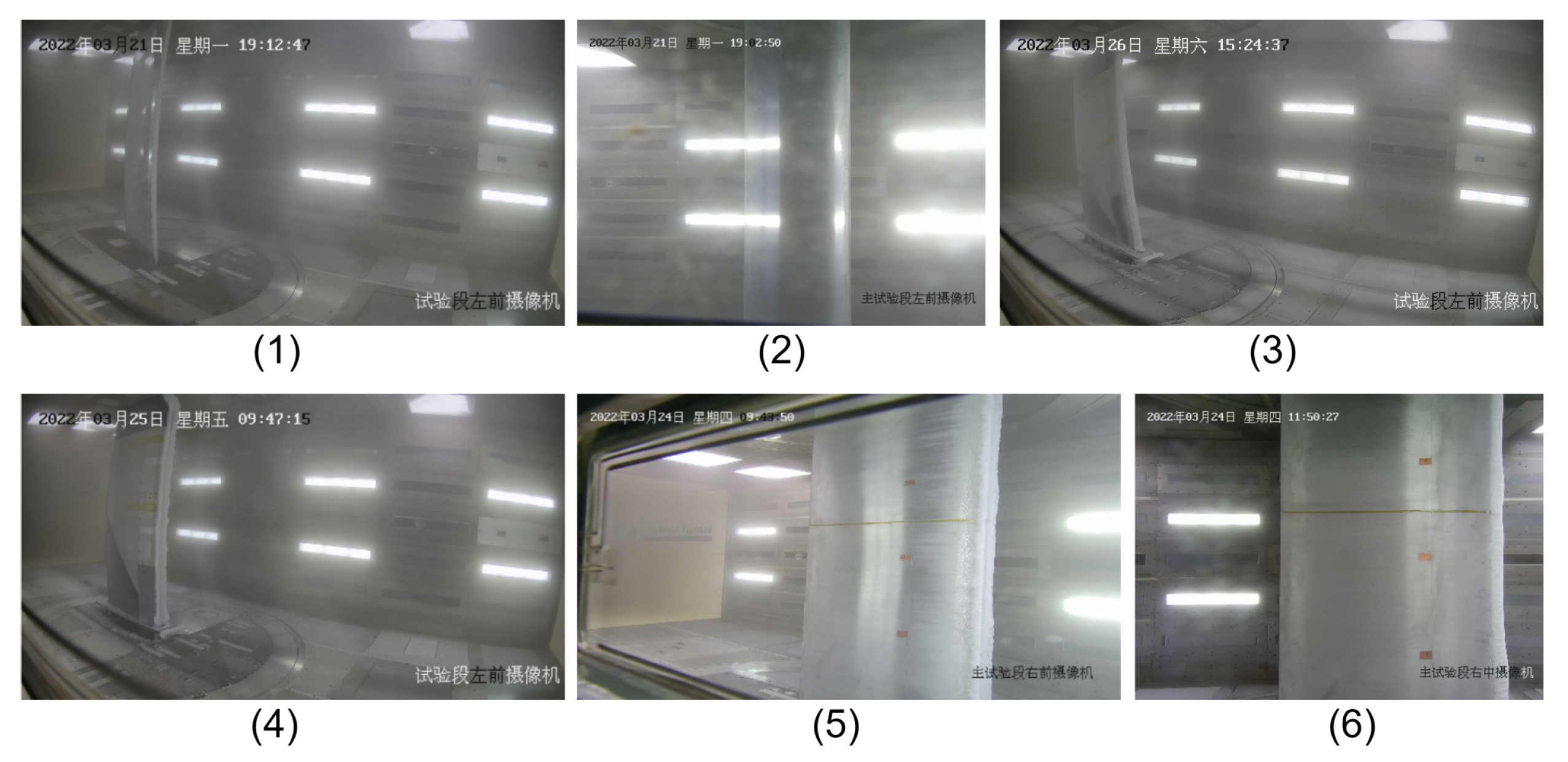
  • We proposed the development of a novel generative image super-resolution dehazing model, which is suitable for the icing wind tunnel environment. We validated the model using real-world images captured in the icing environment, and the results showed excellent dehazing performance.
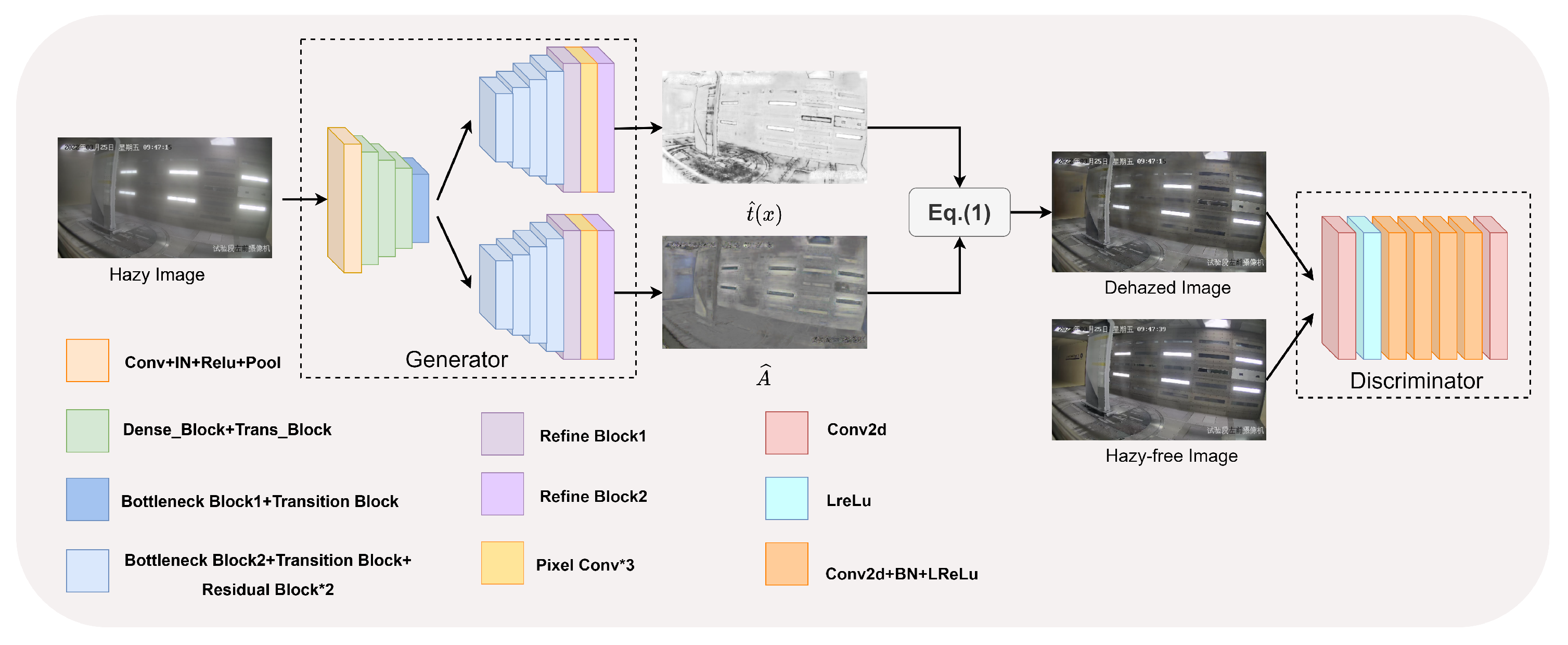
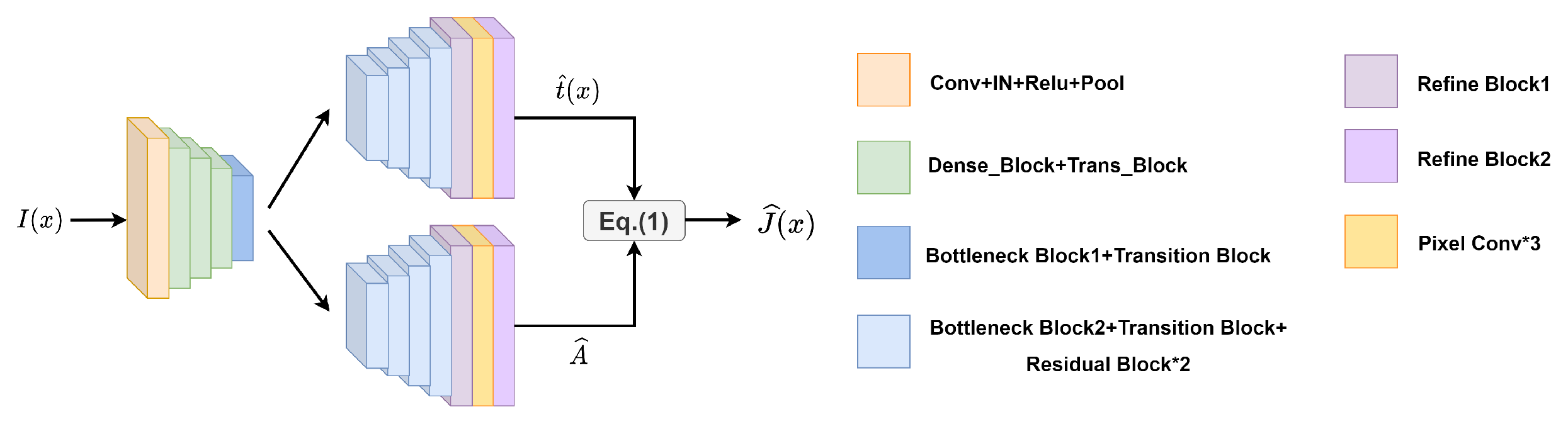
  • The proposed model involves the incorporation of sub-pixel convolution and instance normalization into the network architecture to generate high-resolution dehazed images while preserving the structural information of ice on the wings. Sub-pixel convolution is employed to mitigate artifacts arising from traditional deconvolution, while instance normalization is used to enhance image style transformation. The model enables the capture of both content and style information from hazy and haze-free images, leading to a more effective restoration of the haze-free appearance.

2. Materials and Methods

The entire framework of the proposed network structure is shown in Figure 1. It includes three modules: (1) a generator, which is a network structure estimation to learn the transmittance map t ( x ) and the atmospheric illumination value A; (2) image restoration, which is realized by Equation (2); and (3) a discriminator, which discriminates the dehazed image and its corresponding real haze-free image.

2.1. Generator

The specific network structure of the generator is shown in Figure 2. The left encoder is constructed based on the dense convolutional network (DCN) [15], using the Dense_Block and the Trans_Block in as the main modules. These modules are utilized to extract important features from the image. The right decoder estimates the scene information based on the features extracted from the encoder and restores the image to its original size. The structure of the decoder is similar to that of the encoder, including the bottleneck layer (Bottleneck Block) [13], the transmission layer (Transition Block), the residual layer (Residual Block), and the refinement layer (Refine Block) [8].
In the network architecture, the pre-trained parameters from the front part of DenseNet-201 are used from BaseBlock to the third Trans_Block. This is because the structure in the network can achieve feature reuse by concatenating the obtained features in the channel, and using this connection block in dehazing work helps to preserve important features of the hazy image. In this paper, we replace the batch normalization layer with the instance normalization layer. This modification can normalize the training data and increase the stability of the network during training, thereby avoiding gradient explosion. The Transition Block changes the number of channels through a 1 × 1 convolution layer, reorders the features, and then upsamples the refined features. Additionally, instance normalization layers are used in this block. The residual network adds an identity mapping layer on top of the shallow network, which enables the network to maintain performance as the depth increases. A residual layer is often added after the transition block to extract more high-frequency information and help recover more details in the image. To alleviate the gradient vanishing during network propagation, we also add an instance normalization layer in the residual block. The refinement layer merges image information from different scales. Refine Block1 in Figure 2 extracts local average information of different spatial sizes using the average pooling layer, and then refines the output through a 1 × 1 convolution layer. Subsequently, the sub-pixel convolution is used as the upsampling operation to enlarge the image to the same size. Finally, the locally reassembled images are refined by Refine Block2 to refine image information and remove blocking artifacts.

2.1.1. Instance Normalization

Image dehazing can be regarded as an image style transfer, from the style of an image with haze to the scene of a clear image. The authors of [16] used instance normalization instead of batch normalization in style transfer algorithms. Through experimental comparison, it was proved that this can make the neural network training more stable and reliable. At the same time, instance normalization can also improve the speed of image stylization.
Instance normalization performs independent standardization processing on each feature channel of each sample, which can better preserve the details of the image, and it does not depend on the batch size, making it suitable for small batch training. Based on the specialty of instance normalization, we replaced batch normalization with instance normalization in the network structure. This modification enhances the generalization ability of the dehazing model, resulting in a better dehazing result.

2.1.2. Sub-Pixel Convolution

Sub-pixel convolution [17] is a pixel rearrangement upsampling method that can increase the resolution of low-resolution data to high-resolution space. It is widely used in tasks such as image super-resolution, image deblurring, and image denoising. The sub-pixel convolution process is described as follows:
I H R = f L ( I L R ) = P S ( W L × f L 1 ( I L R ) + b L )
I H R is a high-resolution image, I L R is a low-resolution image, f is a convolution operation, W L is the weight of the convolution kernel, b L is the bias item, and P S is the pixel reorganization operation.
Sub-pixel convolution is an upsampling method based on pixel rearrangement. It can super-resolve low-resolution data to high-resolution space by selecting one element from each channel of the low-resolution feature map and combining them into a new square unit on the high-resolution feature map. In this paper, we replace the original upsampling layer with the sub-pixel convolution layer, which eliminates the need to add meaningless zero elements during the upsampling process and can eliminate the artifacts caused by traditional deconvolution. The sub-pixel convolution layers improve the quality and visual effect of the dehazed image, and then help to reduce computational complexity.

2.2. Image Restoration
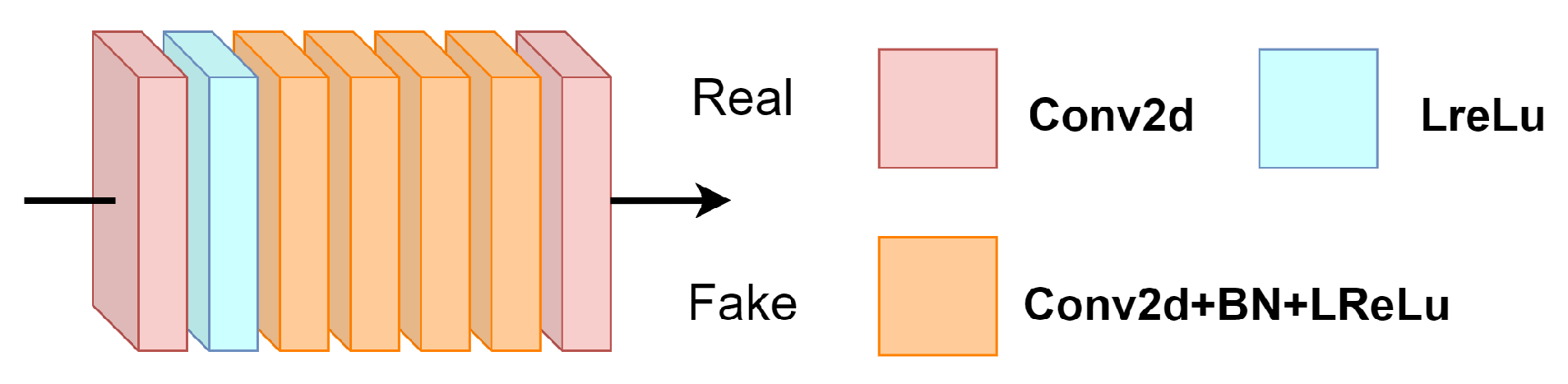
In the generator module, effective estimation of the transmission map t ( x ) and atmospheric light value A is achieved through the encoder–decoder structure, and the dehazed image can be obtained based on Equation (2).

2.3. Discriminator

Here, we use a PatchGAN discriminator structure [18]. This structure divides the input image into several small local blocks, and then evaluates each local block separately before making an overall judgment on the authenticity of the entire image. This approach effectively captures local features in the image and produces higher-resolution dehazed images during model training. Due to the small number of parameters and fast processing speed, PatchGAN can be applied to images of any size. The discriminator is composed of a series of convolutional layers, batch normalization layers and activation layers, as shown in Figure 3.
The main meaning of “Fake” and “Real” in Figure 3 is the discrimination result of the discriminator on the input picture, and whether the picture is a real training image or a fake image from the generator. “Fake” means that the discrimination result is a fake image from the generator, and “Real” means that the discrimination result is a real training image. Through continuous training, the pictures generated by the generator can deceive the discriminator, that is, the discriminator distinguishes the picture as “Real”.

2.4. Loss Function

To better train the network and generate clear images, we use three common losses: reconstruction loss, perceptual loss, and adversarial loss to regulate the learning direction of network parameters during training.

2.4.1. Reconstruction Loss

We use reconstruction loss to measure the difference between the generated dehazed image and the actual dehazed image in the image pixel space, which can be expressed as
L R e s = 1 N i = 1 N | | G ( I i ) J i | | 1
where I i represents the input foggy image, J i represents the real haze-free image corresponding to the image, and G I i represents the dehazing generated by the generator picture.

2.4.2. Perceptual Loss

Here, we also use perceptual loss to measure the perceptual similarity between the dehazed image and the haze-free image in the feature space. Specifically, we evaluate this loss by utilizing the parameters of the pre-trained VGG16 network model.
L p = 1 N i = 1 N | | ϕ ( G ( I i ) ) ϕ ( J i ) | | 2 2
where ϕ . represents the feature map obtained from the VGG16 network layer.

2.4.3. Adversarial Loss

In generative adversarial networks, adversarial loss is one of the most commonly used types of loss to restore the authenticity of the generated images. It uses a binary cross-entropy function to calculate the loss value.
L A = i = 1 N log 1 D J i , G I i

2.4.4. Overall Loss Function

Finally, the haze removal network is regularized by combining the reconstruction loss function, perceptual loss function, and adversarial loss function, which is defined as follows:
L a l l = L Re s + L p + L A

3. Results

3.1. Settings

The hazy images used in this paper were captured from multiple angles in the icing wind tunnel experimental scene supported by the Key Laboratory of Icing and Anti/De-icing of CARDC. To simulate the state of the aircraft passing through the supercooled water droplet cloud layer, the icing wind tunnel experiment can spray a cloud and mist field with a certain median volume diameter (MVD) and liquid water content (LWC) by adjusting the water pressure and air pressure of the nozzle. MVD and LWC are important determining parameters of the haze degree of the cloud and mist field. The data sets we used here include foggy images with an MVD of 25 μm and LWC of 1.31 g/m 3 , MVD of 22 μm and LWC of 1.19 g/m 3 , and MVD of 20 μ m and LWC of 1.0 g/m 3 and 0.5 g/m 3 , respectively. Some samples are shown in Figure 4, and Table 1 presents the MVD and LWC values of the images displayed in the figure.
In this paper, the training set consists of 310 cropped hazy images captured from multiple views in icing wind tunnel experiments. The PyTorch framework is used to train the model, and during training, input images are resized to 1024 × 1024. The Adam optimizer is used to optimize both the generator and discriminator with a learning rate set to 10 4 . A total of 100 epochs are iterated. The experiment is conducted on an environment with a P6000 GPU, 24 GB of memory, and Ubuntu 18.04 operating system.

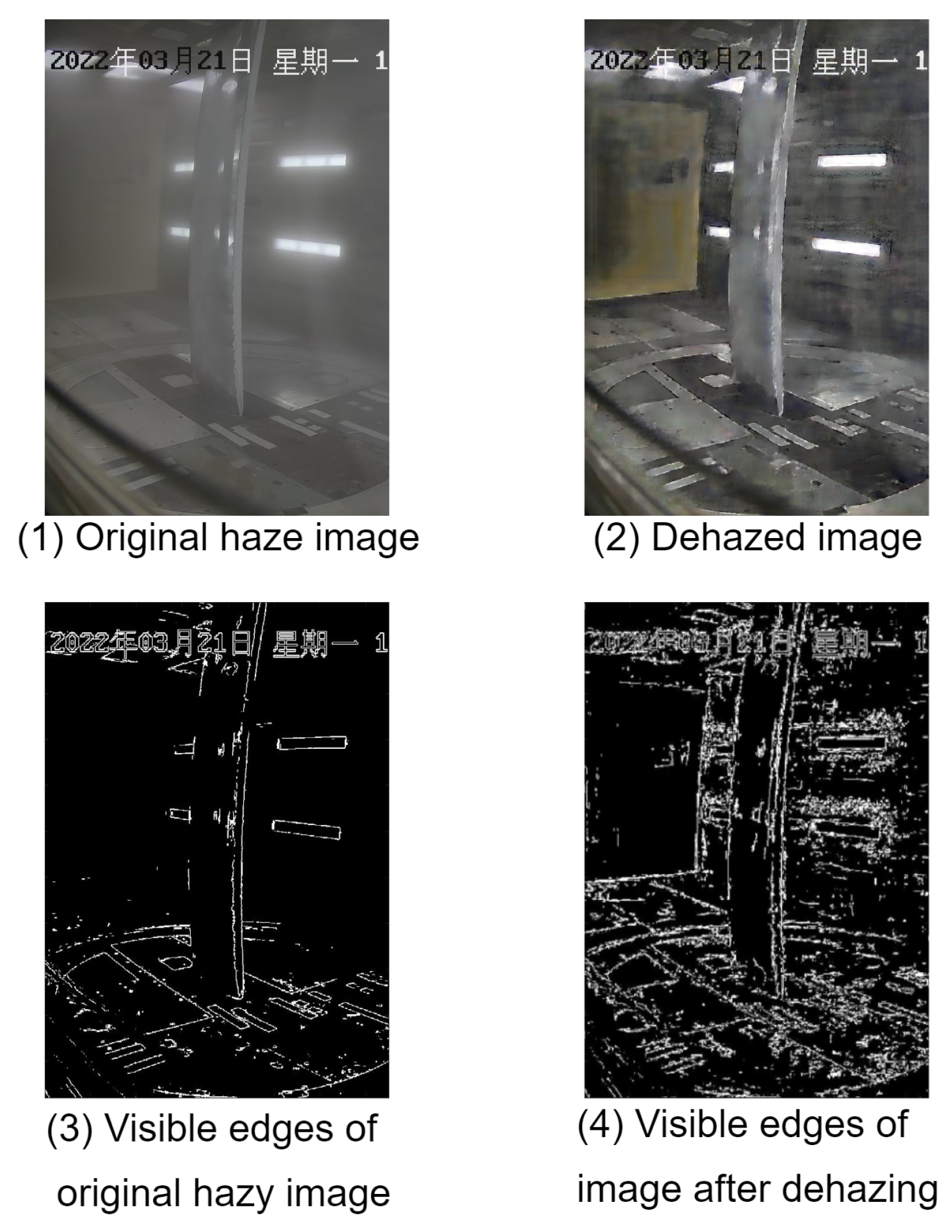
3.2. Evaluation Metrics

The commonly used image quality evaluation metrics include PSNR, SSIM, NIQE [19], visible edge gradient method [20], RRPD [21], LIFQA [22], and DeepSRQ [23], etc.
In the experiment, as we do not have corresponding reference clear images, in order to objectively demonstrate the dehazing effect, we used the widely used visible edge gradient method and NIQE to evaluate the experimental results. The visible edge gradient method has two important indicators: the ratio of visible edges e and the regularized mean visible edge gradient r ¯ . Visible edges are assumed to be those with local contrast greater than 5%. As shown in Figure 5, after defogging, the overall contrast of the image is enhanced and the number of visible edges measured increases.
The relevant expressions are as follows:
e = n r n 0 n 0
n 0 and n r represent the number of visible edges before and after image defogging, respectively, and e represents the ability of the algorithm to restore invisible edges in the image. The larger the value, the better the defogging effect.
r ¯ = e x p ( 1 n r P i Y r log r i )
Y r is the set of pixels on the visible edges of the image after dehazing, r i represents the ratio of gradients at pixel point P i between the defogged image and the foggy image. The larger the value of r ¯ , the higher the contrast of the image after defogging, and the better the effect.
N I Q E calculates the quality score of an image by comparing the statistical properties of the image with those of a high-quality natural image reference set. The expression is as follows:
D ( v 1 , v 2 , 1 , 2 ) = ( ( v 1 ν 2 ) T ( 1 + 2 2 ) 1 ( v 1 ν 2 )
where v 1 , v 2 , 1 , and 1 , respectively, represent the mean vectors and covariance matrices of the natural MVG model and the distorted image MVG model. A smaller N I Q E value indicates better perceived quality.
Due to the defogging operation on the picture in the icing wind tunnel environment, it is necessary to preserve the structure and edge information of the icing wing in the picture to a great extent. So, we pay more attention to the value of the visible edge ratio e and the regularized visible edge gradient mean r ¯ . The e and r ¯ values can more objectively show the number of edges recovered in the image after dehazing.

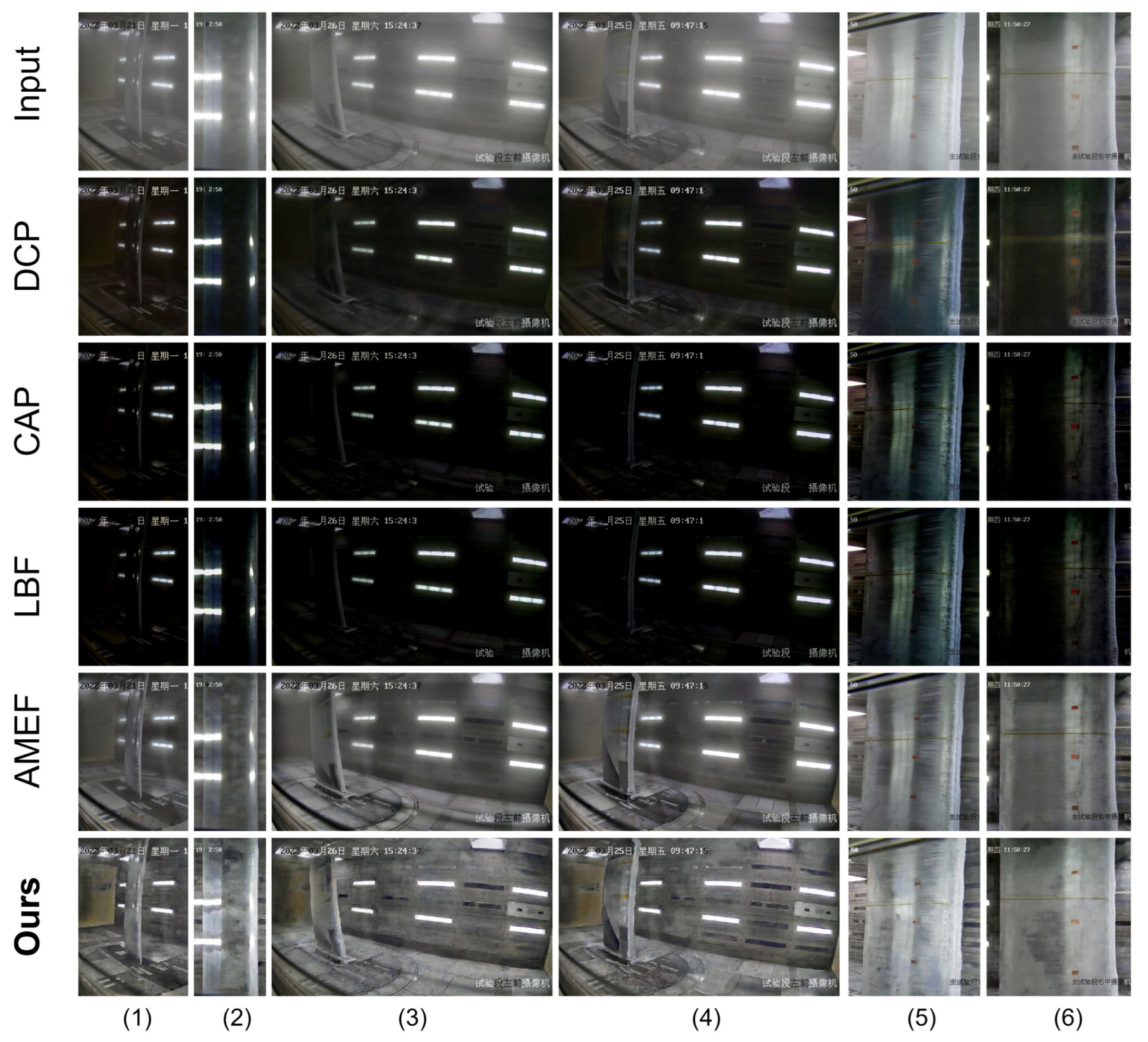
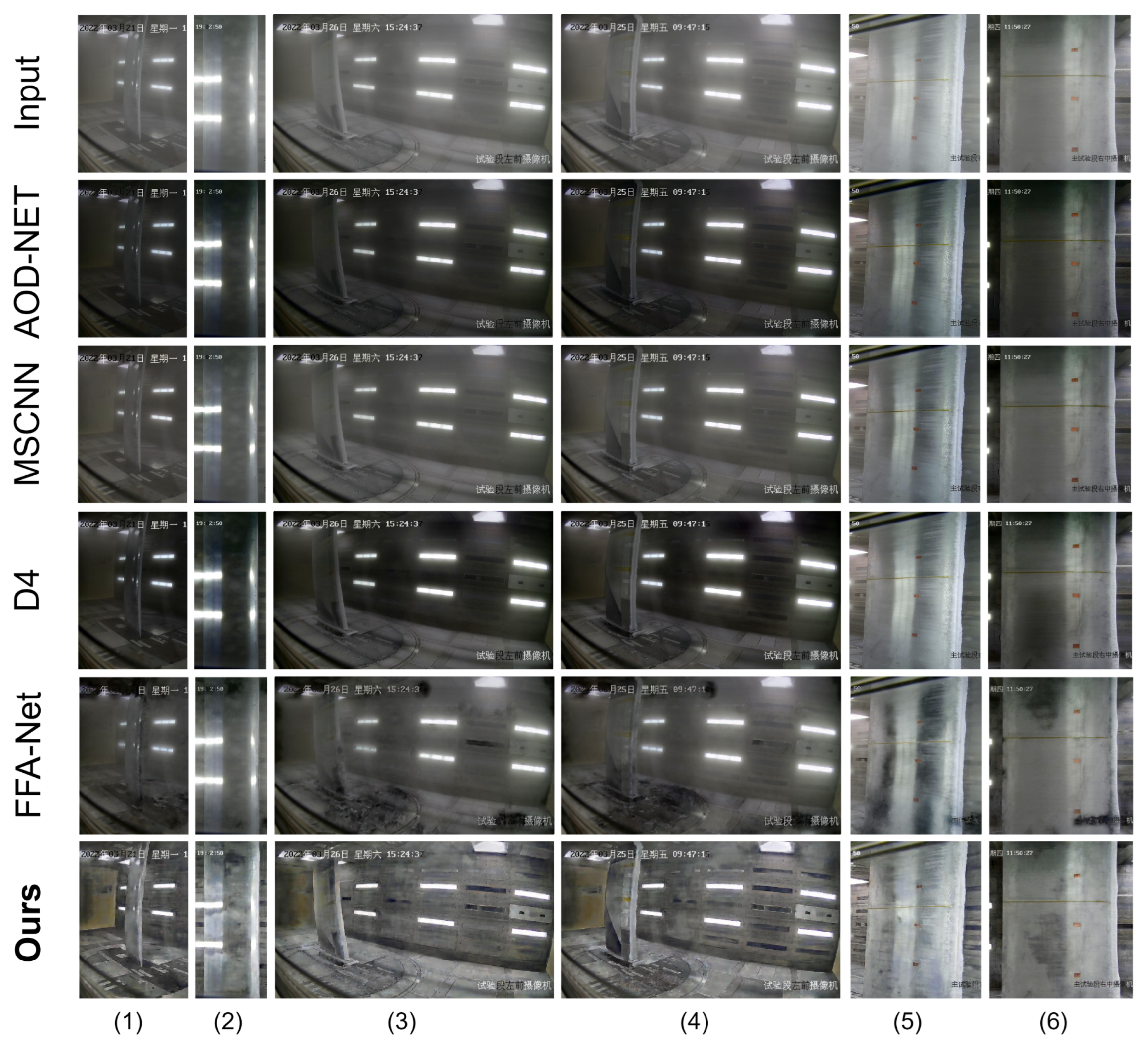
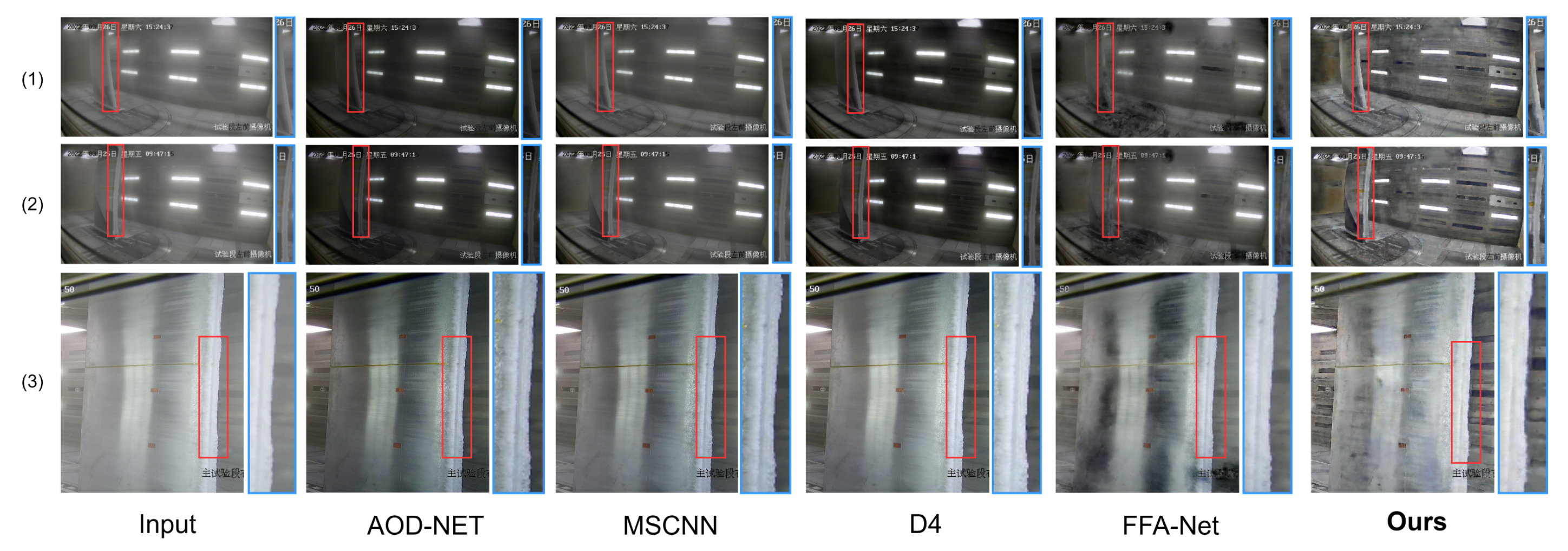
3.3. Comparative Experiments

To evaluate our proposed model more accurately, a comparison with state-of-the-art dehazing methods was performed on icing wind tunnel haze images. Advanced methods include traditional dehazing methods: DCP [2], CAP [3], AMEDF [24], LBF [25]; and deep learning methods: AOD-NET [26], MSCNN [6], FFA-Net [11], D4 [27].
Table 2 shows the comparison results between our model and traditional dehazing methods on the wind tunnel dataset, and Figure 6 shows the corresponding visual comparison. From Figure 6, we can visually observe that DCP, CAP, and LBF have color distortion, and the colors of the dehazed images are very dark. AMEF has a certain dehazing effect, but there is still some residual haze in the dehazed image. According to Table 1, although traditional dehazing methods obtain a higher number of visible edges in the dehazed result, the value of r ¯ needs to be improved. Our model achieves the best result of r ¯ in dense fog situations with an LWC of 1.31 and 1.0, and the value of N I Q E is also smaller. Overall, our model dehazes more thoroughly and has better visual effects.
Table 3 shows the comparison results of our model and deep learning-based methods on the wind tunnel dataset, and the visual comparison of the results after dehazing is shown in Figure 7. From the results, it can be observed that AOD-NET also suffers from color distortion, resulting in darkened colors in the dehazed images. MSCNN has poor dehazing performance, D4 performs well in dehazing the foreground of the images, while FFA-Net destroys the images. In contrast, our model not only has a certain restoration effect on the distant parts of the images, but also better restores the color of the haze-free images. The dehazed images are clearer, and the original contours are preserved. Therefore, a smaller N I Q E value is obtained.

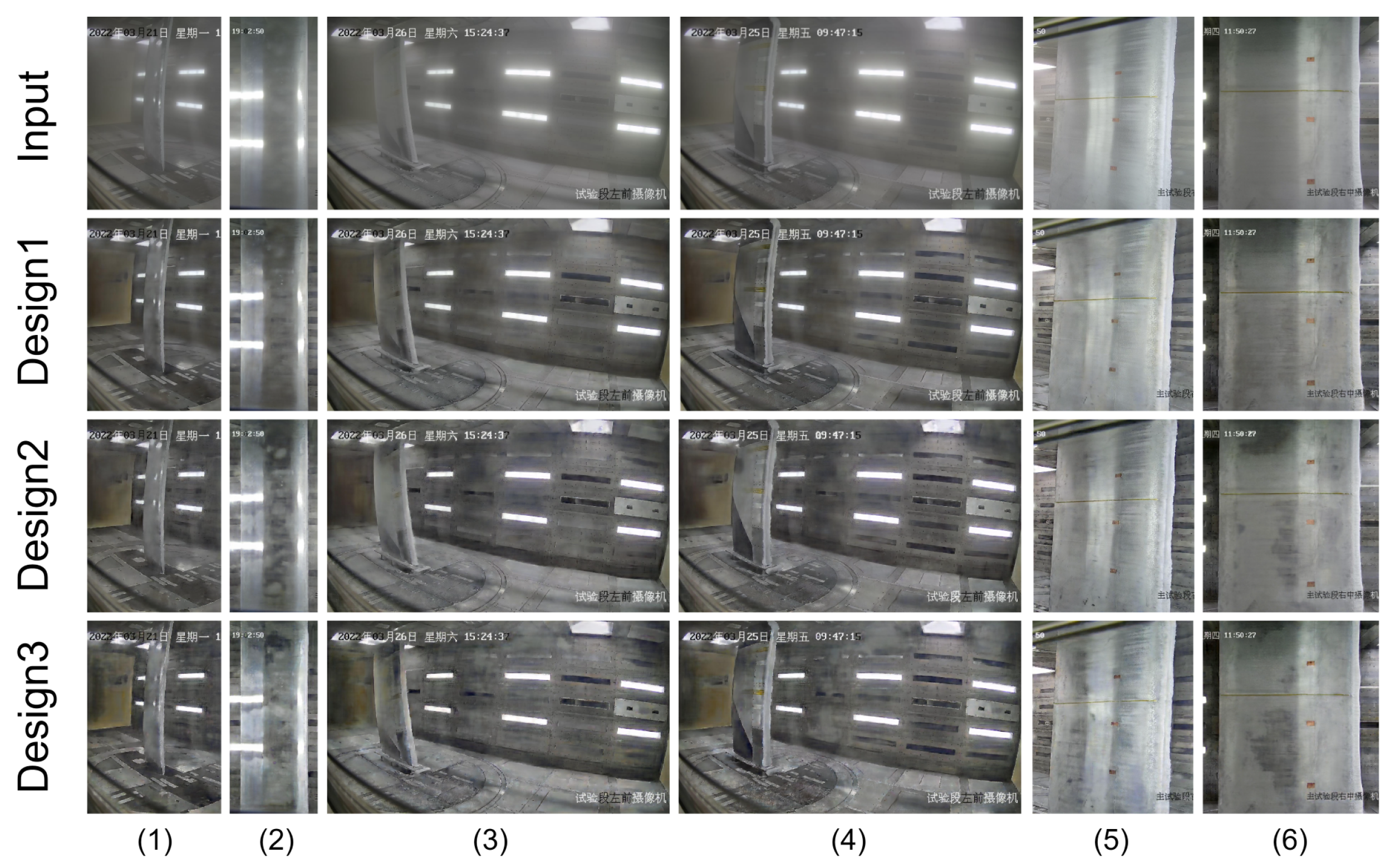
3.4. Ablation Experiments

In this section, we report on ablation experiments conducted on the same test set to analyze the effect of instance normalization and the sub-pixel convolution layer on image dehazing in our method. Three designs are considered: (1) introducing sub-pixel convolution; (2) introducing the instance normalization layer; and (3) using the whole method. All the methods are trained with the same settings as our algorithm for comparison. The experimental results and result images are shown in Table 4 and Figure 8, respectively.
Combining Table 4 and the comparison results in Figure 8, it can be seen that the addition of sub-pixel convolution can better preserve the shape of the ice on the wing edge, while the addition of instance normalization has better dehazing effect. Moreover, Design 2 achieves good results in terms of N I Q E value, and has the best dehazing effect in the case of thin fog with an LWC of 0.5. However, in general, e and r ¯ can more objectively show the number of edges recovered in the image after dehazing. The e and r ¯ values of design 2 are still smaller than those of design 3. Introducing the model with sub-pixel convolution and instance normalization achieves more thorough fog removal, and effectively improves the visible edge count ratio e and the mean visible edge gradient r ¯ , except that the dehazed result of Image 4 has little color distortion.

4. Discussion

To reduce the loss of image information and obtain high-resolution dehazed images in icing wind tunnel environments, we proposed Dense-HR-GAN. Firstly, in the network architecture, the structure of “Dense_Block+Trans_Block” in the encoder part can concatenate the obtained features on the channel. This can achieve the effect of feature reuse and avoiding feature loss. Secondly, using instance normalization in the network structure can independently normalize each feature channel of each sample. This better preserves the details of the image and improves the robustness of the model. Thirdly, the feature maps extracted from the encoder will be skip-connected with those from the decoder. Skip connections can effectively address the problem of deep networks struggling to learn low-level information by connecting shallow feature maps with deep ones, thereby improving the performance and effectiveness of the model. This helps preserve the original important information of the image in the dehazing process.
As analyzed in Section 3.3, our dehazing results are satisfactory, and the evaluation metric r ¯ and N I Q E achieve good values. As shown in Figure 6, compared with traditional dehazing algorithms, our model can better restore the colors of the images and has obvious dehazing effects. Figure 9 shows a partial comparison of our model with a deep learning-based dehazing algorithm. As seen in the third row of images, our model produced dehazed images with higher contrast and more thorough haze removal under LWC = 1.0. Moreover, in the case of LWC = 0.5, our model produced dehazed images that allow for clearer observation of icing on the wings and effectively preserves the original shape of the ice to a great extent, as shown in the red boxed regions in the first two rows of images. (The blue box area is an enlarged version of the red box area in the image).

5. Conclusions

In this paper, we propose a high-resolution dense-connection GAN model called Dense-HR-GAN for dehazing images from an icing wind tunnel environment. The proposed model enhances the clarity of test images to some extent and is beneficial for the subsequent ice shape recognition work. Based on the generative adversarial network framework, we embed the atmospheric scattering model into the network and solve the dehazing problem based on the inverse problem of image formation. In the generator part, we introduced instance normalization and sub-pixel convolution to improve the model’s generalization ability and help eliminate artifacts in the dehazed image, resulting in higher-resolution images. The use of the PatchGAN discriminator helps to obtain more accurate dehazed images. Experimental results on data from the icing wind tunnel show that our method can effectively remove haze and outperform the state-of-the-art techniques. In the future, we would like to continue to optimize our network model to improve the dehazing performance in dense fog conditions.

Author Contributions

Conceptualization, W.Z.; methodology, W.Z.; software, W.Z. and X.Y.; validation, W.Z.; formal analysis, W.Z.; investigation, Y.W.; resources, C.Z.; data curation, X.Y.; writing—original draft preparation, X.Y.; writing—review and editing, W.Z.; visualization, B.P.; supervision, W.Z. and C.Z.; funding acquisition, W.Z. and C.Z. All authors have read and agreed to the published version of the manuscript.

Funding

Supported by the Key Laboratory of Icing and Anti/De-icing of CARDC (Grant No. IADL20210203) and Natural Science Foundation of Sichuan, China, under Grant 2023NSFSC0504.

Institutional Review Board Statement

Not applicable.

Informed Consent Statement

Informed consent was obtained from all subjects involved in the study.

Data Availability Statement

The data used to support the findings of this study are part of a private image data set.

Acknowledgments

The authors would like to acknowledge the following people for their assistance: Zhang Quan, Wei Jiatian, Wang Tianfei, and Wang Shun.

Conflicts of Interest

The authors declare no conflict of interest.

References

  1. McCartney, E.J. Optics of the Atmosphere: Scattering by Molecules and Particles; John Wiley and Sons, Inc.: New York, NY, USA, 1976. [Google Scholar]
  2. He, K.; Sun, J.; Tang, X. Single image haze removal using dark channel prior. IEEE Trans. Pattern Anal. Mach. Intell. 2010, 33, 2341–2353. [Google Scholar] [PubMed]
  3. Zhu, Q.; Mai, J.; Shao, L. A fast single image haze removal algorithm using color attenuation prior. IEEE Trans. Image Process. 2015, 24, 3522–3533. [Google Scholar] [PubMed]
  4. Jobson, D.J.; Rahman, Z.U.; Woodell, G.A. A multiscale retinex for bridging the gap between color images and the human observation of scenes. IEEE Trans. Image Process. 1997, 6, 965–976. [Google Scholar] [CrossRef]
  5. Soni, B.; Mathur, P. An improved image dehazing technique using CLAHE and guided filter. In Proceedings of the 2020 7th International Conference on Signal Processing and Integrated Networks (SPIN), Noida, India, 27–28 February 2020; pp. 902–907. [Google Scholar]
  6. Ren, W.; Liu, S.; Zhang, H.; Pan, J.; Cao, X.; Yang, M.H. Single image dehazing via multi-scale convolutional neural networks. In Proceedings of the European Conference on Computer Vision, Amsterdam, The Netherlands, 11–14 October 2016; pp. 154–169. [Google Scholar]
  7. Cai, B.; Xu, X.; Jia, K.; Qing, C.; Tao, D. Dehazenet: An end-to-end system for single image haze removal. IEEE Trans. Image Process. 2016, 25, 5187–5198. [Google Scholar] [CrossRef]
  8. Zhang, H.; Patel, V.M. Densely connected pyramid dehazing network. In Proceedings of the IEEE Conference on Computer Vision and Pattern Recognition, Salt Lake City, UT, USA, 18–23 June 2018; pp. 3194–3203. [Google Scholar]
  9. Dong, Y.; Liu, Y.; Zhang, H.; Chen, S.; Qiao, Y. FD-GAN: Generative adversarial networks with fusion-discriminator for single image dehazing. In Proceedings of the AAAI Conference on Artificial Intelligence, New York, NY, USA, 7–12 February 2020; Volume 34, pp. 10729–10736. [Google Scholar]
  10. Liu, X.; Ma, Y.; Shi, Z.; Chen, J. Griddehazenet: Attention-based multi-scale network for image dehazing. In Proceedings of the IEEE/CVF International Conference on Computer Vision, Seoul, Republic of Korea, 27 October–2 November 2019; pp. 7314–7323. [Google Scholar]
  11. Qin, X.; Wang, Z.; Bai, Y.; Xie, X.; Jia, H. FFA-Net: Feature fusion attention network for single image dehazing. In Proceedings of the AAAI Conference on Artificial Intelligence, New York, NY, USA, 7–12 February 2020; Volume 34, pp. 11908–11915. [Google Scholar]
  12. Song, Y.; He, Z.; Qian, H.; Du, X. Vision Transformers for Single Image Dehazing. arXiv 2022, arXiv:2109.12564. [Google Scholar] [CrossRef] [PubMed]
  13. Guo, T.; Li, X.; Cherukuri, V.; Monga, V. Dense scene information estimation network for dehazing. In Proceedings of the IEEE/CVF Conference on Computer Vision and Pattern Recognition Workshops, Long Beach, CA, USA, 16–20 June 2019; pp. 2122–2130. [Google Scholar]
  14. Ancuti, C.O.; Ancuti, C.; Sbert, M.; Timofte, R. Dense Haze: A benchmark for image dehazing with dense-haze and haze-free images. arXiv 2019, arXiv:1904.02904v1. [Google Scholar]
  15. Huang, G.; Liu, Z.; Van Der Maaten, L.; Weinberger, K.Q. Densely connected convolutional networks. In Proceedings of the IEEE Conference on Computer Vision and Pattern Recognition, Honolulu, HI, USA, 21–26 July 2017; pp. 4700–4708. [Google Scholar]
  16. Ulyanov, D.; Vedaldi, A.; Lempitsky, V. Instance Normalization: The Missing Ingredient for Fast Stylization. arXiv 2016, arXiv:1607.08022. [Google Scholar]
  17. Shi, W.; Caballero, J.; Huszár, F.; Totz, J.; Aitken, A.P.; Bishop, R.; Rueckert, D.; Wang, Z. Real-time single image and video super-resolution using an efficient sub-pixel convolutional neural network. In Proceedings of the IEEE Conference on Computer Vision and Pattern Recognition, Las Vegas, NV, USA, 27–30 June 2016; pp. 1874–1883. [Google Scholar]
  18. Zhu, J.Y.; Park, T.; Isola, P.; Efros, A.A. Unpaired Image-to-Image Translation using Cycle-Consistent Adversarial Networks. In Proceedings of the 2017 IEEE International Conference on Computer Vision (ICCV), Venice, Italy, 22–29 October 2017. [Google Scholar]
  19. Mittal, A.; Soundararajan, R.; Bovik, A.C. Making a “completely blind” image quality analyzer. IEEE Signal Process. Lett. 2012, 20, 209–212. [Google Scholar] [CrossRef]
  20. Hautiere, N.; Tarel, J.P.; Aubert, D.; Dumont, E. Blind contrast enhancement assessment by gradient ratioing at visible edges. Image Anal. Stereol. 2008, 27, 87–95. [Google Scholar] [CrossRef]
  21. Zhou, W.; Zhang, R.; Li, L.; Liu, H.; Chen, H. Dehazed Image Quality Evaluation: From Partial Discrepancy to Blind Perception. arXiv 2022, arXiv:2211.12636. [Google Scholar]
  22. Zhai, G.; Sun, W.; Min, X.; Zhou, J. Perceptual quality assessment of low-light image enhancement. ACM Trans. Multimed. Comput. Commun. Appl. (TOMM) 2021, 17, 1–24. [Google Scholar] [CrossRef]
  23. Zhou, W.; Jiang, Q.; Wang, Y.; Chen, Z.; Li, W. Blind quality assessment for image superresolution using deep two-stream convolutional networks. Inf. Sci. 2020, 528, 205–218. [Google Scholar] [CrossRef]
  24. Galdran, A. Image dehazing by artificial multiple-exposure image fusion. Signal Process. 2018, 149, 135–147. [Google Scholar] [CrossRef]
  25. Raikwar, S.C.; Tapaswi, S. Lower bound on transmission using non-linear bounding function in single image dehazing. IEEE Trans. Image Process. 2020, 29, 4832–4847. [Google Scholar] [CrossRef] [PubMed]
  26. Li, B.; Peng, X.; Wang, Z.; Xu, J.; Feng, D. Aod-net: All-in-one dehazing network. In Proceedings of the 2017 IEEE International Conference on Computer Vision (ICCV), Venice, Italy, 22–29 October 2017; pp. 4770–4778. [Google Scholar]
  27. Yang, Y.; Wang, C.; Liu, R.; Zhang, L.; Guo, X.; Tao, D. Self-Augmented Unpaired Image Dehazing via Density and Depth Decomposition. In Proceedings of the IEEE/CVF Conference on Computer Vision and Pattern Recognition, New Orleans, LA, USA, 18–24 June 2022; pp. 2037–2046. [Google Scholar]
Figure 1. An overview of the proposed Dense-HR-GAN image dehazing method. It includes a generator and a discriminator. The generator is responsible for generating physical parameters t ^ ( x ) and A ^ . Then, the atmospheric scattering model is inverted to output a dehazed image. Finally, the discriminator discriminates between the dehazed image and the haze-free image.
Applsci 13 05171 g001
Figure 2. Generator. Learning to estimate parameters t ( x ) and A through densely connected networks.
Applsci 13 05171 g002
Figure 3. Discriminator. Driving the generator to capture the local information of the image can be highly advantageous in generating a dehazed image with relatively high resolution.
Applsci 13 05171 g003
Figure 4. Some sample images from the icing wind tunnel. ((16) in the picture represent Image 1 to Image 6).
Applsci 13 05171 g004
Figure 5. Comparison of visible edges before and after dehazing: e = 0.88, r ¯ = 2.91 after dehazing.
Applsci 13 05171 g005
Figure 6. Comparison of six real foggy images in an icing wind tunnel with existing traditional methods. (1,2) LWC = 1.31; (3,4) LWC = 1.0; (5,6) LWC = 0.5.
Applsci 13 05171 g006
Figure 7. Comparison of six real foggy images in an icing wind tunnel with existing deep learning methods. (1,2) LWC = 1.31; (3,4) LWC = 1.0; (5,6) LWC = 0.5.
Applsci 13 05171 g007
Figure 8. Comparison chart of ablation experiment effect. Design 1 means that only sub-pixel convolution is added, Design 2 means that only instance normalization is added, and Design 3 is our proposed model, which adds sub-pixel convolution and instance normalization. ((16) in the picture represent Image 1 to Image 6).
Applsci 13 05171 g008
Figure 9. A partial comparison of our model with a deep learning-based dehazing algorithm. The blue box area is an enlarged version of the red box area in (1,2) LWC = 1.0; and (3) LWC = 0.5.
Applsci 13 05171 g009
Table 1. Display of MVD and LWC values for some icing wind tunnel datasets.
Image 1Image 2Image 3Image 4Image 5Image 6
MVD (μm)252520202020
LWC (g/m 3 )1.311.311.01.00.50.5
Table 2. Comparison of the results of traditional methods on the test set.
MetricImageDCP [2]CAP [3]AMEDF [24]LBF [25]Ours
eImage 11.673.511.591.812.03
Image 26.7314.644.5411.803.47
Image 31.333.361.412.521.31
Image 41.212.351.181.801.82
Image 52.603.122.414.410.64
Image 63.744.982.484.410.52
Average 2.885.332.274.461.63
r ¯ Image 11.221.212.351.194.45
Image 21.161.462.481.845.34
Image 31.041.172.501.243.82
Image 41.131.112.491.174.03
Image 51.341.502.061.942.28
Image 61.241.242.231.471.79
Average 1.191.282.351.483.62
N I Q E Image 13.437.483.457.483.17
Image 22.803.332.813.332.86
Image 33.654.213.304.213.03
Image 43.314.223.104.222.95
Image 53.042.842.882.842.54
Image 63.343.583.703.583.11
Average 3.264.283.214.282.94
Table 3. Comparison of results of deep learning methods on the test set.
MetricImageAOD-NET [26]MSCNN [6]FFA-Net [11]D4 [27]Ours
eImage 12.380.461.301.772.03
Image 25.410.761.405.473.47
Image 31.750.300.861.561.31
Image 41.390.260.631.231.82
Image 52.001.161.401.090.64
Image 62.940.680.721.730.52
Average 2.650.601.052.141.63
r ¯ Image 11.701.221.341.494.45
Image 22.181.291.451.605.34
Image 31.731.201.431.533.82
Image 41.691.191.351.524.03
Image 51.741.371.481.442.28
Image 61.531.151.261.361.79
Average 1.761.241.221.493.62
N I Q E Image 14.314.062.923.993.17
Image 23.553.852.763.412.86
Image 33.783.672.913.543.03
Image 43.563.522.762.322.95
Image 53.253.013.012.992.54
Image 64.243.843.433.843.11
Average 3.783.662.973.352.94
Table 4. Ablation experiment results for modules.
MetricImageDesign 1Design 2Design 3
eImage 10.882.132.03
Image 21.452.153.47
Image 30.821.541.31
Image 40.722.091.82
Image 50.440.910.64
Image 60.630.450.52
Average 0.821.551.63
r ¯ Image 12.914.084.45
Image 23.384.405.34
Image 32.563.633.82
Image 42.603.884.03
Image 52.022.402.28
Image 61.831.851.79
Average 2.553.373.62
N I Q E Image 12.952.813.17
Image 23.092.712.86
Image 33.002.723.03
Image 42.862.612.95
Image 52.802.492.54
Image 63.332.943.11
Average 3.012.712.94
Disclaimer/Publisher’s Note: The statements, opinions and data contained in all publications are solely those of the individual author(s) and contributor(s) and not of MDPI and/or the editor(s). MDPI and/or the editor(s) disclaim responsibility for any injury to people or property resulting from any ideas, methods, instructions or products referred to in the content.

