Featured Application
Autonomous Driving.
Abstract
While detecting surrounding vehicles in autonomous driving is possible with advances in object detection using deep learning, there are cases where small vehicles are not being detected accurately. Additionally, real-time processing requirements must be met for implementation in autonomous vehicles. However, detection accuracy and execution speed have an inversely proportional relationship. To improve the accuracy–speed tradeoff, this study proposes an ensemble method. An input image is downsampled first, and the vehicle detection result is acquired for the downsampled image through an object detector. Then, warping or upsampling is performed on the Region of Interest (RoI) where the small vehicles are located, and the small vehicle detection result is acquired for the transformed image through another object detector. If the input image is downsampled, the effect on the detection accuracy of large vehicles is minimal, but the effect on the detection accuracy of small vehicles is significant. Therefore, the detection accuracy of small vehicles can be improved by increasing the pixel sizes of small vehicles in the transformed image more than the given input image. To validate the proposed method’s efficiency, the experiment was conducted with Argoverse vehicle data used in an autonomous vehicle contest, and the accuracy–speed tradeoff improved by up to a factor of two using the proposed ensemble method.
1. Introduction
Autonomous driving is defined as driving with support from an autonomous driving system controlled by a computer without any external assistance. The possibility of accidents increases when this system cannot accurately detect objects such as vehicles. While improvements have been made to deep learning and deep learning-based object detection techniques [1,2,3,4,5,6], there is still a problem where vehicles far from a camera are not detected accurately [7]. In this study, we denote small (or large) vehicles as faraway (or nearby) for the purpose of explanation because the faraway (or nearby) vehicles from a camera are shown as small (or large) objects in images captured from an autonomous driving system. Additionally, autonomous driving systems should be able to detect vehicles even when another vehicle from the opposite line approaches quickly; therefore, the execution speed [8] should also be considered when applying deep learning-based object detectors to autonomous driving systems.
With many possible solutions to the accuracy problem, using the ensemble method [9,10], studies have been conducted regarding improving the detection accuracy of vehicles [11,12,13,14,15,16,17,18,19,20]. Furthermore, many studies have reported the application of the You Only Look Once (YOLO) network, which is a single-stage Convolutional Neural Network (CNN) [21,22,23,24,25,26,27] that is superior in terms of detection accuracy and execution speed. Regarding this, some studies have reported [28,29,30] the use of the ensemble method on YOLO in a contest of object detection for autonomous driving. However, most of these studies have only focused on the improvement of accuracy or simply using fast detectors, neglecting to consider the tradeoff between detection accuracy and execution speed [31].
This study proposes an ensemble method that accurately detects small vehicles while satisfying the real-time requirement. In this method, the input image is downsampled, and the result of vehicular detection is acquired through the first object detector. Then, perspective transformation (i.e., warping) or upsampling is performed on the Region of Interest (RoI) where the small vehicles are located and applied on the second object detector. Finally, an ensemble method that uses two different object detectors is proposed. The downsampling of the input image does not degrade the detection accuracy of large vehicles. However, the second detector increases the pixel count of small vehicles in the transformed image beyond that in the input image, potentially improving the detection accuracy of small vehicles with faster execution speed.
The accuracy results for the Argoverse dataset [32] divided by vehicle size are listed in Table 1. In this study, small, medium, and large vehicles are not arbitrarily chosen, rather, the 39,343 images of the Argoverse dataset are arranged in the order of vehicle sizes for the Ground Truth (GT) dataset and split into an even 33% ratio for each size, named small, medium, and large. AP0.5 is the Average Precision (AP) value when the Intersection over Union (IoU) of the detection box and GT are more than 0.5, and thus, AP0.5-Small, AP0.5-Medium, and AP0.5-Large mean the accuracy of small, medium, and large vehicles, respectively. As shown in Table 1, the accuracy of small vehicles is relatively low compared to the accuracy of large vehicles; this difference in accuracy increases with a decrease in image resolution. This needs to be focused on to improve the accuracy of overall vehicle detection.

Table 1.
Accuracy results for Argoverse validation data with YOLOv7-Tiny [27]. The accuracy is decreased by 0.16, 0.10, and 0.03 for small, medium, and large vehicles, respectively, with 480 × 320 image resolution, compared to 1920 × 1216.
Figure 1 shows the Ground Truth (GT) of the training images in the Argoverse dataset, which indicates the small vehicles in blue. As visualizing all of the Argoverse GT boxes of small vehicles with one image is difficult, the example shows the small vehicles only for the first 1000 images (shown as blue boxes) on the first Argoverse image. The example shows many small vehicles included in the RoI region. That is, the center region where the small vehicles are located (i.e., shown as a red parallelogram in Warping, a sky-blue rectangle in Upsampling #1, a green rectangle in Upsampling #2) is set as the RoI for the second detector. When drawing boxes for detecting small vehicles for the first 1000 images from the Argoverse dataset, many small vehicles were focused on the center (the red, sky-blue, or green rectangular region can be set to indicate the RoI for small vehicle detection). There are exceptions (outside of the RoIs), but most driving is assumed to occur in a straight line instead of curves (continuous curves are exceptionally rare). If the second detector focuses on the RoI, the accuracy of the small vehicle detector can be improved.
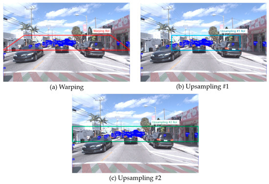
Figure 1.
Illustration of small vehicle distribution for the first 1000 images of the Argoverse dataset.
This study’s contributions are as follows:
- Since the location of the camera in autonomous vehicles is fixed, we assume no height difference is present for the perspective view with either the training or test data. Therefore, we propose acquiring AccumulateImage, which distributes the location of small vehicles from the training dataset, and configuring the RoI with this distribution.
- We acquired the transformed images by either using perspective transformation on the configured RoI or performing upsampling and then identifying the locations of the small vehicles in the box regions. Thus, we propose a method to convert the detection boxes to the coordinates of the RoI region using an inverse perspective transformation.
- Furthermore, we propose an ensemble-based vehicle detection method that considers the requirements of real-time processing. The comparison of the detection results of the two deep learning-based models used in the ensemble method with the baseline reveals that the execution speed of vehicle detection can be improved without degrading the accuracy. To the best of our knowledge, this is the first report of improving the execution speed without degrading the detection accuracy with an ensemble-based vehicle detection method.
The remainder of this study is structured as follows. Section 2 describes the research related to the proposed study. Section 3 describes the proposed method of setting an RoI where small vehicles can be located, detecting small vehicles in the transformed images, and merging the results of the two detectors. Section 4 discusses the experimental results of this study. Finally, in Section 5, the conclusions and scope for future research are discussed.
2. Background
The goal of this study is vehicle detection, which is operated in real-time on an embedded board in an autonomous driving system. Many studies have reported the use of an ensemble method to improve vehicle detection accuracy. For example, some studies [11,12] have reported accuracy improvement by using an ensemble method on SSD [33] and Faster-RCNN [34], YOLOv5 [25], and Faster-RCNN. A different study [13] reported an ensemble method with region-based fully convolutional neural networks R-FCN + YOLOv3, RFCN + RetinaNet, Cascade-RCNN + YOLOv3, and Cascade-RCNN [35] + RetinaNet. The results of an ensemble method were shown with residual networks ResNet-50 and SE-ResNeXt-50 [14]. Using the ensemble method, the detection accuracy has not only been improved in the vehicular environment but also in the field of unmanned aerial vehicles (UAVs) [15,16,17]; other studies have [18,19,20] also reported improvements in the detection accuracy using the concept of ensemble models. However, common aspects of these reported studies include the execution time not being reported or reductions in the execution speed after implementing the ensemble method. Therefore, other studies have reported on the application of the ensemble method using the one-stage CNN-based object detector YOLO [21,22,23,24,25,26,27], which considers the execution time of the autonomous driving system. For example, there have been studies [28,29,30] wherein real-time processing results have been obtained by applying the ensemble method to a YOLO-based object detector model on a V100 graphical processing unit (GPU). The results obtained using the proposed methods in previous studies are for expensive GPU environments; autonomous driving systems require processing in a low-cost GPU environment [31].
Previous studies in the last five years that have improved the accuracy of vehicle detection using the ensemble method are summarized in Table 2. The studies can be grouped as either using top-view, tilted-view, or side-view images. Additionally, many studies have solely focused on improving the accuracy, and as a result, have neglected to report the inference time and not specify whether the test was processed in a CPU/GPU environment. The current study utilized object size differences in side-view images, as in autonomous vehicles, instead of top/tilted-view and regions in which small vehicles appear. The proposed method also takes the execution speed on low-cost embedded boards into consideration.
Table 2.
Some of the preceding studies (“ensemble”, “vehicle”, and “detection” included in the title) were published between 2018 and 2022. No prior results on the use of ensemble methods in vehicle detection with execution speed improvement have been reported. Execution time below 30 ms per image needs to be satisfied for real-time processing.
To summarize, an input image is downsampled, and then the detection result is acquired by applying a downsampled image to a fast object detector (i.e., first deep learning model A focusing on large vehicles). Additionally, the RoI, where small vehicles are present, undergoes perspective transformation or upsampling and is inputted into another fast object detector (i.e., second deep learning model B focusing on small vehicles). We propose an ensemble method that merges the results of these two detection models. Compressing the input image has almost no impact on the detection accuracy of large vehicles but has an impact on the detection accuracy of small vehicles. Increasing the number of pixels on a small vehicle beyond that in the original input image using the transformed image may improve the overall detection accuracy with faster execution speed.
3. Proposed Method
The purpose of this study is to support vehicle detection in an autonomous driving environment. No height difference is assumed to be present for the training dataset and test dataset as the camera installed within the vehicle is fixed. Additionally, classes categorized as Car, Bus, and Truck are changed to a Vehicle class, and images without a Vehicle class are excluded. Additionally, the accuracy of vehicle detection differs between small/medium/large vehicles in terms of image resolution, as shown in Table 1. For given input images (e.g., 1920 × 1216), this study proposes applying the detection results of the downsampled images (e.g., 960 × 608) obtained using the first detector (defined as Model A, shown in Figure 2) and the detection results of the transformed images (e.g., 1920 × 320 or 3840 × 320) obtained using the second detector (defined as Model B, shown in Figure 2) as inputs to the merging phase to improve the detection accuracy of small vehicles with faster execution speed. That is, Model A is a baseline model (i.e., YOLOv7-tiny) for downsampled images, while Model B is a modified YOLOv7-tiny model for transformed images. Section 3.1 discusses the configuration of the RoI for Model B. Then, in Section 3.2, the acquisition of the detection result from Model B is discussed. Finally, Section 3.3 discusses merging the results of Model A with the results of Model B.
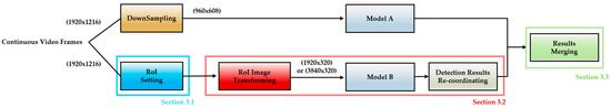
Figure 2.
Illustration of a Proposed Method for 1920 × 1216 Images. After creating a downsampled image, we apply Model A (YOLOv7-tiny) to obtain the detection result A. Then, an RoI is acquired to improve the small vehicle accuracy, and a transformed image is acquired with the RoI. The transformed image is applied to Model B (modified YOLOv7-tiny) to obtain the detection result B. Since the object’s location shifted greatly from the original image with the transformation, detection result B is recalibrated and combined with detection result A.
3.1. Setting RoI Configuration for Model B
Visualizing all of the Argoverse GT boxes of 39,343 training images into corresponding small, medium, and large vehicles is difficult due to overlapping boxes. Therefore, Figure 3 shows images containing GT boxes in the training data by selecting each group of 1000 images for small, medium, and large vehicles to visualize each location. Small and medium vehicles are generally located at the center of the image in terms of the y-axis, whereas large vehicles appear in various locations of the image.
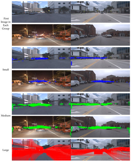
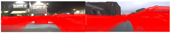
Figure 3.
Illustrations of four groups of Argoverse training data (i.e., each group shows the GT boxes for 1000 images). In each group, small, medium, and large images show the distribution of small, medium, and large GT boxes with different colors on the first image of each group. The blue boxes (for small vehicles) and the green boxes (for medium vehicles) are generally located at the center of the image in terms of the y-axis. On the other hand, the red boxes (for large vehicles) are distributed at various locations in the image.
Figure 4 shows the results of accumulating the number of boxes for each pixel position using 39,343 images of training data, assigning the maximum pixel value of 255 (white) containing the largest number of boxes, and assigning the rest of the pixels as a value between 0 and 255 based on that value. For example, each pixel position with a grey value of 255 (i.e., white) in AccumulateImage_S means the most frequent position for small vehicles. By creating AccumulateImage, as shown in Figure 4, the RoI region is configured for the second detector Model B, used for small vehicle detection (see Figure 1 and Algorithm 1). Accordingly, the RoI region is configured on AccumulateImage_S to detect small vehicles, a transformed image is generated, and the transformed image is applied to the second detector Model B (Section 3.2).
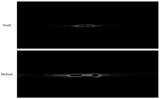
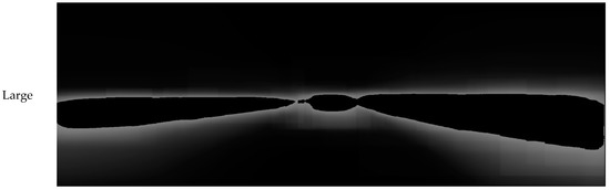
Figure 4.
AccumulateImage_S, AccumulateImage_M, AccumulateImage_L showing the distribution of small, medium, and large vehicles for 39,343 Argoverse training data.
The total computational workloads for Model A and Model B are set to be less than that of the baseline model. Additionally, the resolution of the transformed image is configured to be a multiple of 32 under the assumption that a CNN-based detector including YOLO is used. For example, the input image resolution of the baseline model is changed from 1920 × 1200 to 1920 × 1216. Then, the resolution of Model A is set to 960 × 608, and the resolution for Model B is set to 1920 × 320 or 3840 × 320, respectively. To set the resolution of a transformed image under Model B to 320 in terms of the y-axis, the RoI to which perspective transformation or upsampling will be applied is obtained from the 160-pixel range, where the sum of AccumulateImage_S is the maximum from the entire y-axis range. The algorithm for deciding the RoI is shown as Algorithm 1.
| Algorithm 1 RoI Set |
| Input: AccumulateImage_S = Pixel information representing the frequency of small box appearances accumulated in video. Frame = Pixel information for the current frame from the video Output: RoIImage = Pixel information for RoI region through AccumulateImage_S from the original image |
| AccumulateImage_S.rows = rows from AccumulateImage_S AccumulateImage_S.cols = columns from AccumulateImage_S Frame.rows = rows from Frame Frame.cols = columns from Frame Max_sum = 0 RoI_cols = 0 X_Range_1 = AccumulateImage_S.rows/4 X_Range_2 = AccumulateImage_S.rows ∗ 3/4 i = 0 while i < (AccumulateImage_S.cols-160) sum = 0 for x = X_Range_1 to X_Range_2 do for y = i to (i + 160) do sum += AccumulateImage_S[Frame.cols ∗ y ∗ 3 + x ∗ 3] sum += AccumulateImage_S[Frame.cols ∗ y ∗ 3 + x ∗ 3 + 1] sum += AccumulateImage_S[Frame.cols ∗ y ∗ 3 + x ∗ 3 + 2] if Max_sum < sum then Max_sum = sum RoI_cols = i i = i + 160 for x = 0 to Frame.rows/2 do for y = 0 to 160 do RoIImage[160 ∗ y ∗ 3 + x ∗ 3] = Frame[Frame.cols ∗ (y + RoI_cols) ∗ 3 + (x + AccumulateImage_S.rows/2) ∗ 3] RoIImage[160 ∗ y ∗ 3 + x ∗ 3 + 1] = Frame[Frame.cols ∗ (y + RoI_cols) ∗ 3 + (x + AccumulateImage_S.rows/2) ∗ 3 + 1] RoIImage[160 ∗ y ∗ 3 + x ∗ 3 + 2] = Frame[Frame.cols ∗ (y + RoI_cols) ∗ 3 + (x + AccumulateImage_S.rows/2) ∗ 3 + 2] return RoIImage |
While it may seem unusual to use the statistics (i.e., AccumulateImage_S) of the training data in this way, in YOLO [23,24,25,26,28], the anchor size is determined by the statistics of the training data, and the position of the camera mounted on the autonomous vehicle is fixed; therefore, it is assumed that there is no difference in the gaze height between the training and test data, which is a natural setting. To summarize, the statistics of the images obtained from the cameras installed in a car and a bus may be different, making it necessary to learn a model specialized for each vehicle.
3.2. Obtaining Detection Results from Transformed Image
A transformed image, as shown in Figure 5, is generated using the RoI region configured from Algorithm 1. First, the transformed image’s y-axis range is set to the previously acquired RoI region, and the x-axis range is set to the entire image. Thus, the range resolution is set to 1920 × 160, and Perspective Transformation (i.e., Warping) is performed on the image, which outputs 1920 × 320. Additionally, the transformed image with Upsampling #1 is applied with the pre-acquired RoI region, and the size of the image is expanded by two. This process upsamples 960 × 160 resolution images into 1920 × 320. The reason for setting the x-axis range differently with two pre-processing methods is that the object shape does not change in the image as Upsampling #1 simply enlarges the RoI region, but the distortion effect occurs with objects, as shown in Figure 5, with the warping image processing method. On the other hand, Warping RoI is configured to be larger than Upsampling #1 RoI in terms of the x-axis range, which may enlarge more objects. Upsampling #2, which expands the x-axis range with upsampling, is additionally considered to compare the accuracy–speed tradeoff.
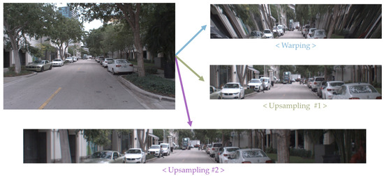
Figure 5.
Transformed images were obtained by three pre-processing methods (Perspective Transformation, Upsampling #1, and Upsampling #2). Different RoIs contain various features when using different pre-processing methods. Warping enlarges the RoI region with perspective transformation. Upsampling #1 simply enlarges the RoI region by two, which increases the object pixel information. Upsampling #2 enlarges the x-axis more than Upsampling #1 to improve the detection accuracy in the larger RoI region.
Next, the detection result is acquired with the second detector Model B. The proposed method modifies the network structure of the baseline model differently, as shown in Figure 6, to improve the accuracy–speed tradeoff for small vehicles. In general, CNN-based object detectors, including YOLO, have a backbone consisting of Stage 1~Stage 5, a neck consisting of Stage 3~Stage 5, and three heads focusing on small, medium, and large object detection. Figure Structure 1 removing the Stage 5 head focusing on large vehicles and improving the execution speed of the baseline model. Figure 6 Structure 2 shows that the Stage 2 neck affecting the detection accuracy of small vehicles in order to improve the accuracy of Structure 1. Figure 6 Structure 3 is expected to improve the detection accuracy of small vehicles by directly connecting the Stage 2 backbone to the Stage 2 head. Figure 6 Structure 4 is combines Structure 2 and Structure 3 by adding the Stage 2 neck and the Stage 2 head. Figure 6 Structure 5 is a modified version of Figure 6 Structure 4, with the connection from the Stage 2 neck to the Stage 3 neck deleted.
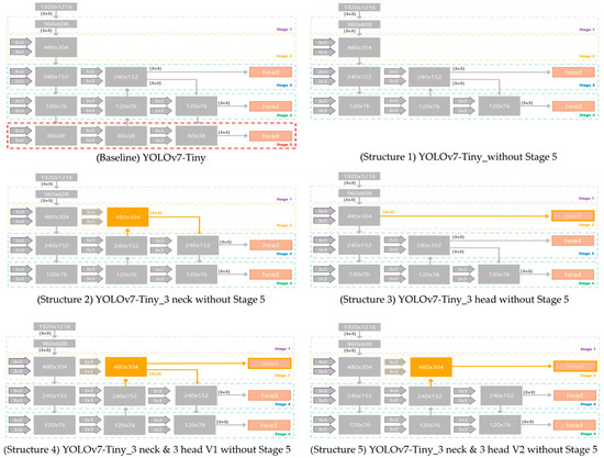
Figure 6.
Illustration of various network structures for Model B of 1920 × 1216 input images (accuracy–speed tradeoff considered). Structure 1 removes Stage 5, which has a significant impact on large vehicle accuracy. While the accuracy decreases by removing Stage 5, the speed is improved. Further modifications are made to supplement the reduced accuracy caused by Structure 1, even though the speed may be degraded. For example, Structure 2 adds the Stage 2 neck to Structure 1, whereas Structure 3 adds the Stage 2 head to Structure 1. Both Structure 4 and Structure 5 combine Structure 2 and Structure 3, with a difference in the connection from the Stage 2 neck to the Stage 3 neck.
Finally, since the detection result of Model B is acquired from a transformed image, the detection result needs a post-processing method that inverses the detection result to merge with the detection result of Model A. That is, detection results from the input images and the transformed images are different, as image pre-processing is performed to improve the detection accuracy of small and medium vehicles. Therefore, the detection result of Model B is re-coordinated in order to match the detection result from the transformed image to the input image’s vehicle size. In addition, the pixel information that is overlapped with the RoI configured in Figure 3 can be lost, as shown in Figure 5. Hence, the detection information is not included within certain regions configured by the pre-processing method. The algorithm of the second phase is shown as Algorithm 2.
| Algorithm 2 Re-coordinate the detections |
| Input: Frame = Pixel information for the current frame from the video Model B = Network Modified Model Warping_Coordinates = Two coordinates on the image to apply Perspective Transformation on: [y1, y2] Checking the pre-processing method = 0(upsampling#1 or upsampling#2), 1(warping) RoIImage = Pixel information for RoI region through AccumulateImage_S from the original image Output: Re-coordinate_Detections = Box list readjusted from Model B to the original image |
| Perspect_Mat // 3 × 3 array used when warp transforming, saved only once in the first frame. if Checking the pre-processing method = 0 then // Image transformation is performed using the RoI image obtained from Algorithm 1. Upsampling1_Frame = Upsampling1_Transform(Frame, RoIImage) // Box list for the present Upsampling1_Frame from Model B Detections_B_U_1 = GetBoxList(Upsampling1_Frame, Model_B) // The box information detected through image conversion is readjusted to match the original image. Re-coordinate_Detections = Upsampling1Re-adjustment(Detections_B_U_1, Frame) return Re-coordinate_Detections else if Checking the pre-processing method == 1 then // Image transformation is performed using the RoI image obtained from Algorithm 1. Upsampling2_Frame = Upsampling2_Transform(Frame, RoIImage) // Box list for the present Upsampling2_Frame from Model B Detections_B_U_2 = GetBoxList(Upsampling2_Frame, Model_B) // The box information detected through image conversion is readjusted to match the original image. Re-coordinate_Detections = Upsampling2Re-adjustment(Detections_B_U_2, Frame) return Re-coordinate_Detections else if Perspect_Mat.data = 0 then // When there is no value of Inverse_Perspect_Mat Frame_p[0] = [W/3, Warping_Coordinates[y1]] Frame_p[1] = [W * 2/3, Warping_Coordinates[y1]] Frame_p[2] = [0, Warping_Coordinates[y2]] Frame_p[3] = [W, Warping_Coordinates[y2]] dst_p[0] = [0, 0] dst_p[1] = [W, 0] dst_p[2] = [0, H ∗ 4/5] dst_p[3] = [W, H ∗ 4/5] Perspect_Mat = getPerspectiveTransform(Frame_p, dst_p) // Image transformation is performed using the RoI image obtained from Algorithm 1. Warping_Frame = Warping_Transform(Frame, RoIImage, Perspect_Mat) // Box list for the present Warping_Frame from Model B Detections_B_W = GetBoxList(Warping_Frame, Model_B) // The box information detected through image conversion is readjusted to match the original image. Re-coordinate_Detections = WarpingRe-adjustment(Detections_B_W, Frame, Perspect_Mat) return Re-coordinate_Detections |
3.3. Merging Detection Results from First and Second Detectors
Finally, the detection results of Model B for the post-processed image obtained through Algorithm 2 and the detection results of Model A should be merged. The Intersection over Union (IoU) is not suitable for checking the accuracy of the detection results since it measures only the degree of overlap; thus, the Distance Intersection over Union (DIoU), which considers the center coordinates of the detection results, is used. In the proposed method, if the detection results of each detector are higher than 0.2, then based on the confidence score, only the detection results with a higher confidence score are left, and the other results are removed. The RoI obtained from Algorithm 1 is the configured region, where the possibility of small vehicles being present is high. Therefore, by increasing the confidence score of the results detected within the RoI region of the second detector, the priority is given to the second detector Model B over the first detector Model A. Algorithm 3 shows the pseudo-code for the merging phase.
| Algorithm 3 Merging Detection Results |
| Input: Frame = Pixel information for the current frame from the video Original_Detections = Box list for the current frame from Model A Re-coordinate_Detections = Box list readjusted from Model B to the original image DIoU_Thresh = Variables to determine the degree to which DIoU overlaps the detection results of both models Output: Final_Detections = Final detection results for the current frame |
| //sort first_box and second_box in descending order of confidence value Sort_Descending(Original_Detections) Sort_Descending(Re-coordinate_Detections) matched_boxes = 0 for i = 0 to size of Re-coordinate_Detections do for j = 0 to size of Original_Detections do max_DIoU = largest DIoU of Re-coordinate_Detections[i] and Original_Detections[j] if max_DIoU > DIoU_Thresh do Final_Detections[matched_boxes] = Re-coordinate_Detections[i] Final_Detections[matched_boxes].confidence = Re-coordinate_Detections[i].confidence > Original_Detections[j].con fidence ? Re-coordinate_Detections[i].confidence: Original_Detections[j].confidence matched_boxes++ Original_Detections[j] = 0 for j = 0 to size of Original_Detections do if Original_Detections[j] == 0 then continue Final_Detections[matched_boxes] = Original_Detections[j] matched_boxes++ return Final_Detections |
4. Experimental Results
4.1. Experimental Setup
In this study, cars, trucks, and buses of various (total of 8) classes were set as the target objects in autonomous driving competitions conducted using Argoverse data. All Argoverse data were collected using the same car (i.e., a Ford Fusion Hybrid) fully integrated with Argo AI power generation technology. Annotations are automatically generated throughout an entire tracking sequence. That is, if the full spatial extent of an object is ambiguous in one frame, information from previous or later frames can be used to constrain the shape. Since we focused on the task of 2D object detection, we only used the center RGB camera from multiple sensors. That is, 39,343 images of learning data were set for training and validation (5-fold cross-validation), and 14,572 images of verification data were used for testing. The details of the Argoverse data can be found in [32]. The deep learning model was trained on a PC with an AMD Ryzen 5950× 16-core processor, GeForce RTX 3090 GPU, and 32 GB of RAM. Regarding the specification for training the model, the number of iterations was 30,000, the learning rate was 0.00261, and the anchor box was classified as 9 anchors using the k-means algorithm.
The accuracy of the proposed method was evaluated using the following metrics, where TP is true positive, FP is false positive, and FN is false negative:
- Precision, defined as TP/(TP + FP), means the false detection rate of the proposed method;
- Recall, defined as TP/(TP + FN), means the missed detection rate of the proposed method;
- AP0.5, defined as the average precision (AP) evaluated for vehicle class, means the target accuracy of the proposed method when the IoU of the detection box and the GT is more than 0.5.
Additionally, a recently reported tiny version of YOLOv7 was applied and implemented to consider real-time processing on a low-cost commercial GPU. Particularly, rather than deriving the results optimized for a specific detector on a specific GPU, we assumed a general setup that considered the tradeoff between detection accuracy and execution speed for vehicle detection. In other words, lightweight techniques, such as pruning and quantization, were not applied.
4.2. Detection Performance
Generally, an ensemble method focuses solely on improving the accuracy compared to the baseline model by using multiple and different models. On the other hand, this study proposes an integrated performance of AP0.5 × FPS that determines the cost-effectiveness. This integrated performance focuses on the accuracy–speed tradeoff instead of the prior ensemble method’s purpose (i.e., accuracy only). Additionally, experiments, following the proposed pre-processing methods, of the ‘Ensemble-Warping’, ‘Ensemble-Upsampling #1′, and ‘Ensemble-Upsampling #2′ versions were conducted. The CPU pre-processing time was pipelined by having it processed, while Model A was processed by a GPU. Therefore, execution speed reduction caused by image processing was alleviated.
Table 3 shows an accuracy–speed comparison of various Model B structures for small vehicle detection, as shown in Figure 6. There are many metrics to show accuracies such as Precision, Recall, and AP0.5. In the experiment, AP0.5 was chosen as the target accuracy metric, as it is most often used for object detection accuracy. Additionally, FPS was chosen as the target speed metric, which is a metric measuring the execution speed with frames per second. The structure that showed the highest FPS was Structure 1, as Stage 5 was removed from the baseline model with nothing added. Compared to the baseline model, the FP was decreased, whereas the FN was increased. Although AP0.5 was degraded, the highest FPS of Structure 1 could provide the best AP0.5 × FPS among the five possible structures for Model B. By adding the Stage 2 neck to Structure 1 in Structure 2, the FP of Structure 2 was increased (i.e., degraded Precision), whereas the FN of Structure 2 was decreased (i.e., improved Recall), compared to Structure 1. Although Structure 2 could provide better AP0.5 than Structure 1, the integrated performance of Structure 2 was worse than that of Structure 1 due to the low speed. Note that AP0.5 is the precision metric, and thus, a higher AP0.5 does not guarantee a higher recall rate. On the other hand, in Structure 3, the FP of Structure 3 was decreased, whereas the FN of Structure 3 was increased, compared to Structure 1. Although Structure 3 connected the Stage 2 backbone to the new Stage 2 head directly, the AP0.5 of Structure 3 was worse than that of Structure 1 due to the insufficient high-level information in the Stage 2 backbone. Since both Structure 4 and Structure 5 combined Structure 2 and Structure 3, they had similar accuracy and speed. In summary, this study focused on improving the accuracy–speed tradeoff. Therefore, Structure 1 (i.e., the removal of Stage 5 from the baseline showing the highest integrated performance AP0.5 × FPS) was selected as the final structure for Model B.
Table 3.
Accuracy–speed performance comparison for Model B using a PC GPU (RTX 3090) of 1920 × 1216 input images. Structure 1 showing the highest integrated performance AP0.5 × FPS was selected as the final structure for Model B. The arrows in the table mean that the higher the direction the arrow is, the higher the value.
A performance comparison of the baseline and proposed method of the 1920 × 1216 input image is shown in Table 4. The proposed method using Upsampling #1 could provide the same accuracy as the baseline. On the other hand, the FPS execution speed that measured the total time, including pre-processing and post-processing, increased from 28.80 to 44.80. Hence, the integrated performance of AP0.5 × FPS that measured the target efficiency increased from 23.32 to 36.28, and thus, we denote the proposed method using Upsampling #1 as EnsembleVehicleDet. While we expected the larger effect of a larger RoI on the accuracy by configuring Warping and Upsampling #2 compared to Upsampling #1 in terms of the x-axis, the detection accuracy was slightly lower (0.80 vs. 0.81) or there was no difference (0.81 vs. 0.81) compared to Upsampling #1, respectively. The FPS also showed a slight decrease (44.60 vs. 44.80) or a significant decrease (30.60 vs. 44.80) compared to Upsampling #1. The object density around the center of the image was high in AccumulateImage_S, showing the distribution of small vehicles. While the TP on small vehicles was slightly increased by detecting large regions in terms of the x-axis, the medium and large vehicles’ FP within the y-axis range was also increased, which resulted in overall accuracy degradation. The distortion caused by the perspective transformation was assumed to have a greater effect on the accuracy compared to setting the RoI larger. While partially turning at an intersection (hence, small vehicles located outside of the RoI region) in the test dataset was included, the overall accuracy degradation was minimal. Therefore, the two versions of the proposed methods do not seem to have any problem with integration practically.
Table 4.
Accuracy–speed performance comparison using a PC GPU (RTX 3090) of 1920 × 1216 input images. EnsembleVehicleDet could improve the accuracy–speed tradeoff (i.e., AP0.5 × FPS) of the baseline from 23.32 to 36.28.
Figure 7 (Upsampling #1), Figure A1 (Upsampling #2, see Appendix A), and Figure A2 (Warping, see Appendix A) show the experimental results of the ensemble effect for three images out of the test dataset’s video sequences. In Figure 7, Figure A1, and Figure A2, the first image shows two vehicles parked on the right side of the main road, in addition to many vehicles on the main road. The second image shows a vehicle parked on the left, in addition to many vehicles on the main road. Lastly, the third image shows a vehicle parked on the left, a vehicle parked on the right, and many vehicles on the main road. From left to right, the Model A (first detector) results, Model B (second detector) results within the RoI, and the ensemble results are shown. As shown in Figure 7, Ensemble-Upsampling #1 could solve three FN errors in the first image, three FN errors in the second image, and one FN error in the third image. Similarly, Ensemble-Upsampling #2 could solve three FN errors in the first image, two FN errors in the second image, and one FN error in the third image (see Figure A1 in Appendix A). On the other hand, Ensemble-Warping generated one FP error in the first image while solving one FN error in the first image, two FN errors in the second image, and two FN errors in the third image (see Figure A2 in Appendix A). Note that, as shown in Table 4, all three ensemble methods could provide similar AP0.5, although Ensemble-Upsampling #2 had the lowest speed due to the larger RoI.
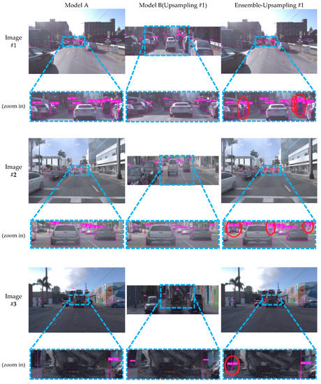
Figure 7.
Comparison of Model A, Model B (Upsampling #1), and Ensemble-Upsampling #1 results. With Ensemble-Upsampling #1, three FN errors in the first image, three FN errors in the second image, and one FN error in the third image were solved (shown as red circles).
Table 5 shows a performance comparison for input images of 960 × 608. Unlike prior experiments, the experiment was performed on an NVIDIA Jetson AGX Xavier board [36] with TensorRT (16-bit floating point). If the 960 × 608 resolution was decreased to 480 × 320, the detection accuracy of the baseline model for small vehicles was decreased from 0.63 to 0.51, and the detection accuracy of medium vehicles was decreased from 0.75 to 0.66, as shown in Table 1. To solve this degradation of detection accuracy for both small and medium vehicles, the experiment was conducted by configuring the RoI y-axis relatively wider for Model B. The integrated performance of the baseline was increased from 36.34 to 68.24 with EnsembleVehicleDet (i.e., Upsampling #1). We expected the effect of the larger RoI on the accuracy by setting the x-axis range wider for Warping and Upsampling #2 compared to Upsampling #1. However, the experiment showed lower accuracy and slower speed than Upsampling #1.
Table 5.
Accuracy–speed performance comparison using an Embedded GPU (AGX board) of 960 × 608 input images (with TensorRT). EnsembleVehicleDet could improve the accuracy–speed tradeoff (i.e., AP0.5 × FPS) of the baseline from 36.34 to 68.24.
Finally, different research issues, such as pruning and quantization, were not applied to focus on the effect of the ensemble method. Utilizing these lightweight techniques, real-time processing, even on a low-cost embedded board, can be expected.
5. Conclusions
The study proposes an ensemble method that improves the accuracy–speed tradeoff for vehicle detection. The input image is downsampled and then inserted into the fast object detector to acquire the vehicle detection results (first detector Model A). The RoI region that contains small vehicles is processed with perspective transformation or upsampling to acquire the detection result (second detector Model B). Then, the detection boxes acquired from the second detector are re-coordinated to the location of the first detector. The second detector is prioritized over the first detector during the merging phase when the final boxes are chosen.
The proposed method was implemented by applying a tiny version of YOLOv7 to satisfy the real-time requirements. The experiment was performed with the Argoverse vehicle dataset, which was used in an autonomous driving contest. The experimental results of a PC GPU (RTX 3090) showed improvement in the detection accuracy of small vehicles without degrading the detection accuracy of large vehicles. From the possible five structures, Structure 1 (i.e., the removal of Stage 5 from the baseline) improved the integrated performance AP0.5 × FPS of the baseline from 23.32 to 26.32 for 1920 × 1216 input images, and thus, it was selected as the final structure for Model B. In addition, we applied a downsampled image to Model A, applied a transformed image to Model B, and then ensembled the detection results from A and B to further increase the accuracy–speed tradeoff. Overall, the vehicle detection accuracy–speed tradeoff was shown to improve from 23.32 to 36.28 for 1920 × 1216 input images. Using an embedded GPU (AGX board) with TensorRT, however, the proposed method could improve the accuracy–speed integrated performance significantly from 36.34 to 68.24 for 960 × 608 input images.
While there is a limitation to using the proposed method for curves in an intersection, most vehicles are assumed to drive straight rather than curved, which shows that this is not such a large shortcoming; overall, the proposed method can still improve the accuracy. Future studies should focus on pedestrians that are smaller than vehicles in object detection.
Author Contributions
D.P. and Y.C. conceptualized and designed the experiments; S.Y., S.S., H.A., H.B. and K.N. designed and implemented the detection system; H.B. and H.A. validated the proposed method; S.Y. and S.S. wrote the paper. All authors have read and agreed to the published version of the manuscript.
Funding
This patent is the result of a local government–university cooperation-based regional innovation project (2021RIS-004), carried out with the support of the Korea Research Foundation with the funding of the Ministry of Education in 2021.
Institutional Review Board Statement
Not applicable.
Informed Consent Statement
Not applicable.
Data Availability Statement
Not applicable.
Conflicts of Interest
The authors declare no conflict of interest.
Appendix A

Figure A1.
Comparison of Model A, Model B (Upsampling #2), and Ensemble-Upsampling #2 results. With Ensemble-Upsampling #2, three FN errors in the first image, two FN errors in the second image, and one FN error in the third image were solved (shown as red circles).

Figure A2.
Comparison of Model A, Model B (Warping), and Ensemble-Warping results. With Ensemble-Warping, one FN error in the first image, two FN errors in the second image, and two FN errors in the third image were solved (shown as red circles), although one FP error was generated in the first image (shown as a brown circle).
References
- Bengio, Y.; Lecun, Y.; Hinton, G. Deep Learning for AI. Commun. ACM 2021, 64, 58–65. [Google Scholar] [CrossRef]
- Li, Z.; Liu, F.; Yang, W.; Peng, S.; Zhou, J. A Survey of Convolutional Neural Networks: Analysis, Applications, and Prospects. IEEE Trans. Neural Netw. Learn. Syst. 2022, 33, 6999–7019. [Google Scholar] [CrossRef]
- Bhatt, D.; Patel, C.; Talsania, H.; Patel, J.; Vaghela, R.; Pandya, S.; Modi, K.; Ghayvat, H. CNN Variants for Computer Vision: History, Architecture, Application, Challenges and Future Scope. Electronics 2021, 10, 2470. [Google Scholar] [CrossRef]
- Dai, H.; Huang, G.; Zeng, H.; Zhou, F. PM2.5 Volatility Prediction by XGBoost-MLP Based on GARCH Models. J. Clean. Prod. 2022, 356, 131898. [Google Scholar] [CrossRef]
- Dai, H.; Huang, G.; Zeng, H.; Yu, R. Haze Risk Assessment Based on Improved PCA-MEE and ISPO-LightGBM Model. Systems 2022, 10, 263. [Google Scholar] [CrossRef]
- Zhao, Z.; Zheng, P.; Xu, S.; Wu, X. Object Detection with Deep Learning: A Review. IEEE Trans. Neural Netw. Learn. Syst. 2019, 30, 3212–3232. [Google Scholar] [CrossRef]
- Wang, Z.; Zhan, J.; Duan, C.; Guan, X.; Lu, P. A Review of Vehicle Detection Techniques for Intelligent Vehicles. IEEE Trans. Neural Netw. Learn. Syst. 2022, 23, 1–21. [Google Scholar] [CrossRef]
- Li, M.; Wang, Y.; Ramanan, D. Towards Streaming Perception. In Proceedings of the ECCV, Glasgow, UK, 23–28 August 2020. [Google Scholar]
- Casado-García, Á.; Heras, J. Ensemble Methods for Object Detection. In Proceedings of the ECAI, Santiago de Compostela, Spain, 29 August–8 September 2020. [Google Scholar]
- Ahn, H.; Son, S.; Kim, H.; Lee, S.; Chung, Y.; Park, D. EnsemblePigDet: Ensemble Deep Learning for Accurate Pig Detection. Appl. Sci. 2021, 11, 5577. [Google Scholar] [CrossRef]
- Mittal, U.; Chawla, P.; Tiwari, R. EnsembleNet: A Hybrid Approach for Vehicle Detection and Estimation of Traffic Density based on Faster R-CNN and YOLO Models. Neural Comput. Appl. 2023, 35, 4755–4774. [Google Scholar] [CrossRef]
- Mittal, U.; Chawla, P. Vehicle Detection and Traffic Density Estimation using Ensemble of Deep Learning Models. Multimed. Tools Appl. 2022, 82, 10397–10419. [Google Scholar] [CrossRef]
- Hai, W.; Yijie, Y.; Yingfeng, C.; Xiaobo, C.; Long, C.; Yicheng, L. Soft-Weighted-Average Ensemble Vehicle Detection Method Based on Single-Stage and Two-Stage Deep Learning Models. IEEE Trans. Intell. Veh. 2021, 6, 100–109. [Google Scholar]
- Sommer, L.; Acatay, O.; Schumann, A.; Beyerer, J. Ensemble of Two-Stage Regression Based Detectors for Accurate Vehicle Detection in Traffic Surveillance Data. In Proceedings of the AVSS, Auckland, New Zealand, 27–30 November 2018. [Google Scholar]
- Darehnaei, Z.; Fatemi, S.; Mirhassani, S.; Fouladian, M. Ensemble Deep Learning Using Faster R-CNN and Genetic Algorithm for Vehicle Detection in UAV Images. IETE J. Res. 2021, 29, 1–10. [Google Scholar] [CrossRef]
- Darehnaei, Z.; Fatemi, S.; Mirhassani, S.; Fouladian, M. Two-level Ensemble Deep Learning for Traffic Management using Multiple Vehicle Detection in UAV Images. Int. J. Smart Electr. Eng. 2021, 10, 127–133. [Google Scholar]
- Jagannathan, P.; Rajkumar, S.; Frnda, J.; Divakarachari, P.; Subramani, P. Moving Vehicle Detection and Classification using Gaussian Mixture Model and Ensemble Deep Learning Technique. Wirel. Commun. Mob. Comput. 2021, 2021, 5590894. [Google Scholar] [CrossRef]
- Walambe, R.; Marathe, A.; Kotecha, K.; Ghinea, G. Lightweight Object Detection Ensemble Framework for Autonomous Vehicles in Challenging Weather Conditions. Comput. Intell. Neurosci. 2021, 2021, 5278820. [Google Scholar] [CrossRef]
- Rong, Z.; Wang, S.; Kong, D.; Yin, B. A Cascaded Ensemble of Sparse-and-Dense Dictionaries for Vehicle Detection. Appl. Sci. 2021, 11, 1861. [Google Scholar] [CrossRef]
- Darehnaei, Z.; Shokouhifar, M.; Yazdanjouei, H.; Fatemi, S. SI-EDTL Swarm Intelligence Ensemble Deep Transfer Learning for Multiple Vehicle Detection in UAV Images. Concurr. Comput. Pract. Exp. 2022, 34, e6726. [Google Scholar]
- Redmon, J.; Divvala, S.; Girshick, R.; Farhadi, A. You Only Look Once: Unified, Real-Time Object Detection. In Proceedings of the CVPR, Las Vegas, NV, USA, 27–30 June 2016. [Google Scholar]
- Redmon, J.; Farhadi, A. YOLO9000: Better, Faster, Stronger. In Proceedings of the CVPR, Honolulu, HI, USA, 21–26 July 2017. [Google Scholar]
- Redmon, J.; Farhadi, A. Yolov3: An Incremental Improvement. arXiv 2018, arXiv:1804.02767. [Google Scholar]
- Bochkovskiy, A.; Wang, C.; Liao, H. Yolov4: Optimal Speed and Accuracy of Object Detection. arXiv 2020, arXiv:2004.10934. [Google Scholar]
- Ultralytics/Yolov5. Available online: https://github.com/ultralytics/yolov5 (accessed on 25 June 2020).
- Ge, Z.; Liu, S.; Wang, F.; Li, Z.; Sun, J. Yolox: Exceeding Yolo Series in 2021. arXiv 2021, arXiv:2107.08430. [Google Scholar]
- Wang, C.; Bochkovskiy, A.; Liao, H. YOLOv7: Trainable Bag-of-Freebies Sets New State-of-the-Art for Real-Time Object Detectors. arXiv 2022, arXiv:2207.02696. [Google Scholar]
- Zhang, Y.; Song, X.; Bai, B.; Xing, T.; Liu, C.; Gao, X.; Wang, Z.; Wen, Y.; Liao, H.; Zhang, G.; et al. 2nd Place Solution for Waymo Open Dataset Challenge—Real-Time 2D Object Detection. In Proceedings of the CVPRW, Nashville, TN, USA, 19–25 June 2021. [Google Scholar]
- Nikolay, S. 3rd Place Waymo Real-Time 2D Object Detection: YOLOv5 Self-Ensemble. In Proceedings of the CVPRW, Nashville, TN, USA, 19–25 June 2021. [Google Scholar]
- Jeon, H.; Tran, D.; Pham, L.; Nguyen, H.; Tran, T.; Jeon, J. Object Detection with Camera-Wise Training. In Proceedings of the CVPRW, Nashville, TN, USA, 19–25 June 2021. [Google Scholar]
- Balasubramaniam, A.; Pasricha, S. Object Detection in Autonomous Vehicles: Status and Open Challenges. arXiv 2022, arXiv:2201.07706. [Google Scholar]
- Argoverse-HD. Available online: https://www.kaggle.com/datasets/mtlics/argoversehd (accessed on 23 September 2022).
- Liu, W.; Anguelov, D.; Erhan, D.; Szegedy, C.; Reed, S.; Fu, C.; Berg, A. SSD: Single Shot Multibox Detector. In Proceedings of the ECCV, Amsterdam, Netherlands, 8–16 October 2016. [Google Scholar]
- Ren, S.; He, K.; Girshick, R.; Sun, J. Faster R-CNN: Towards Real-Time Object Detection with Region Proposal Networks. In Proceedings of the NeurIPS, Long Beach, CA, USA, 4–9 December 2017. [Google Scholar]
- Cai, Z.; Vasconcelos, N. Cascade R-CNN: Delving into High Quality Object Detection. In Proceedings of the CVPR, Salt Lake City, UT, USA, 18–22 June 2018. [Google Scholar]
- NVIDIA 2020. Jetson AGX Xavier Series: Thermal Design Guide. Available online: https://tinyurl.com/r7zeehya (accessed on 23 September 2022).
Disclaimer/Publisher’s Note: The statements, opinions and data contained in all publications are solely those of the individual author(s) and contributor(s) and not of MDPI and/or the editor(s). MDPI and/or the editor(s) disclaim responsibility for any injury to people or property resulting from any ideas, methods, instructions or products referred to in the content. |
© 2023 by the authors. Licensee MDPI, Basel, Switzerland. This article is an open access article distributed under the terms and conditions of the Creative Commons Attribution (CC BY) license (https://creativecommons.org/licenses/by/4.0/).