Improving Landslide Susceptibility Assessment through Frequency Ratio and Classification Methods—Case Study of Valencia Region (Spain)

Featured Application

Two methods are proposed here to improve the reliability of landslide susceptibility maps in risk assessment: (1) Frequency Ratio uses clusters/regression from inventory data, instead of standard intervals and (2) Diagnostic tests improve conventional classifications by considering inventory data.

Abstract

Landslide susceptibility maps are widely used in land management and urban planning to delimit potentially problematic areas. In this article we improve their reliability by acting on the frequency ratio method and map classification systems. For the frequency ratio method, we have worked with continuous variables and established intervals grouped by probability according to the landslide inventory and based on the characteristics of the data rather than on standard divisions. For map classification systems, we have compared the efficacy of conventional classifications and those based on the concepts of sensitivity and specificity, with the specificity classifications being supported by the information offered by available comparative data. Both strategies make it possible to avoid subjective and repetitive procedures that are alien to the nature of the data being assessed. We present a case study in the 23,000 km² Region of Valencia where a total of 48 different susceptibility maps were generated. We demonstrate that the methods applied in this study to calculate the frequency ratio provide an improvement in specificity in areas of high susceptibility while maintaining good sensitivity. In particular, the Area Under Curve (AUC) values increase from 0.67 for the conventional methods to 0.76 with the methods proposed in this work. This improvement is transferred to susceptibility mapping much more clearly when classifications that incorporate sensitivity, and especially specificity parameters, are used.

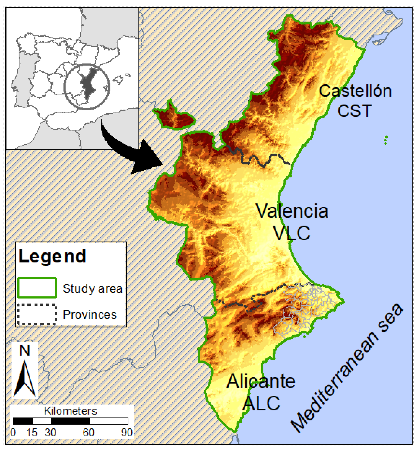
1. Introduction

Landslide susceptibility maps (LSM) are valuable and necessary resources for deciding how land should be planned, particularly in mountainous areas. Different techniques and methods for determining susceptibility have been developed since the 1970s, including classic statistical, index-based, and machine learning methods [1]. GIS technology is a useful tool for managing and analysing spatial data in relation to landslides [2,3].

Table 1. Methods for Landslide Susceptibility Assessment [4,5].

Methods	Description	Advantages	Disadvantages
Knowledge (opinion)-driven: - AHP - Analytic Network process	Ranking and weighting factors by means of experts	Better knowledge processes in the field Do not require large amount of data Expert knowledge contribution	Subjectivity of experts. Qualitative based No consistent standard rules Difficult quantifying results
Bivariate: - Frequency Ratio - Weight of Evidence - Fuzzy logic - Information value - GIS matrix method	Assess environmental characteristics Use terrain factors: slope, geology	Useful for regional scale Quantitative approach Straightforward to implement Easy to understand Satisfactory prediction performance	Certain irrationality in the distribution of weights Generally, less predictive accuracy than multivariate methods Difficult to include a large number of factors
Machine learning (multivariate): - Logistic regression - Artificial neural network - Support Vector Machine - Maximum entropy	Analyse the correlation of landslide—causative factors by means of algorithms Assumption of certain factors or conditions exhibiting similar patterns of landslide	Useful for regional scale Quantitative approach Normally algorithms offer high predictive accuracy Large number of methods	Complicated express underlying rules Use complex algorithms Sensitive to controlling factors Can’t calculate spatial relationship of landslide locations/factors Black box nature No rule of thumb for applying the best method
Physically based (deterministic approach)	Mechanism and landslide processes Geotechnical parameters Analyse slope stability	More exact Strong landslide warning ability Quantitative approach	Requires large amount of data and field survey Small regions Needs homogeneity in ground conditions

shows description advantages and disadvantages of the different techniques used.

Historical landslide inventory data have been fundamental in the preparation of these maps. These data are generally used as contrasts for validation elements to adjust susceptibility values, and especially to establish the levels or classes of the variables that govern the ground-motion mechanisms. This is the case of the ‘frequency ratio method’ (FR). However, it is sometimes felt that these inventory data could be better exploited. In other words, they could provide a better fit in the case of continuous variables, as well as in the mapping classification of susceptibility values.

The likelihood of landslides in a particular area has been widely evaluated using the frequency ratio (FR) method [6,7]. This is a type of bivariate statistical analysis technique that allows for representing landslide susceptibility maps that link the individual factors governing landslide failure to the sensitivity of its occurrence. FR can be easily integrated into a GIS system due to the simplicity of its principles, making it user-friendly [8,9]. However, other methods have proven to be more effective, which highlights the need to improve the FR technique [10,11]. The initial step in using the FR method to analyse landslides (as well as other bivariate methods) is identifying and grouping the factors that contribute to them, such as the angle of the slope and the type of rock, among others. The likelihood of a landslide occurring in a specific area is determined by the numbers and threshold limits of the classes of factors. Determining the thresholds that lead to best results constitutes a major challenge, because it relies on expert knowledge of the area in question and is therefore subjective [12,13,14,15]. One proposal is to use procedures capable of extracting the maximum information from the available data. This paper proposes a method that objectively considers the nature of the inventory data to determine the number of classes and their limits for numerical variables.

The commonly used factor classifications induce discontinuities in the FR values. This implies significant breaks between classes, which will eventually lead to a discontinuity in the spatial distribution of landslide susceptibility. Furthermore, the choice of factor class boundaries is subjective. Therefore, it is of key importance to apply new methods to avoid data gaps and subjective decisions.

Creating clear and easy-to-understand maps is an important aspect of mapping landslide susceptibility. However, grouping data into a set number of classes can have a negative impact on the accuracy of the results, depending on how the classes are defined. Thus, changing the boundaries between classes can lead to vastly different maps [16]. Therefore, the overall accuracy of the classified map is crucial for determining its usefulness in decision-making tasks [17,18]. To assess the reliability of a map for a particular application, it is necessary to make meaningful and consistent measurements of its accuracy. Currently, there are no standard guidelines for classifying landslide susceptibility maps, such as the number and names of classes or class boundaries. Some authors use expert criteria to divide the susceptibility histogram into categories [19,20], which cannot be automated or statistically tested [21], and do not consider the real underlying data. Because of the above, it can be concluded that there is no universally accepted method for classifying landslide susceptibility maps.

Some of these subjects are addressed in the new system for classification methods for susceptibility maps proposed by Cantarino et al. (2019) [22] and based on receiver operating characteristic (ROC) analysis. The authors compare this classification with other standard classification systems (natural breaks, quantiles, head/tail breaks) and demonstrate its greater effectiveness in a mountainous area of about 1500 km². This paper compares this ROC-based method with other classification procedures. One of these procedures also uses the definitions of the ROC space, in particular of sensitivity, but without specificity. This is the European Landslide Susceptibility Map (ELSUS) [23]. The previously mentioned natural breaks and quantiles classification methods are also included to check which is the most reliable method for assessing risk in large areas (as is the study area selected for this work).

In short, the aim of this article is to propose new working procedures together with the adjustment of existing procedures, basing these procedures on a better exploitation of the inventory data. This should lead to an improvement in obtaining and spatially defining risk values for landslide susceptibility maps.

2. Case Study of the Valencia Region

2.1. Description of Study Area

The area selected for the comparative study is the Region of Valencia. This region is in the southeast of Spain (Figure 1) by the Mediterranean Sea. It consists of three provinces—Castellon (CST), Valencia (VLC), and Alicante (ALC)—and includes 542 municipalities. The area covers 23,260 km² and represents 4.60% of the national surface; it had a population of 5,072,000 inhabitants in the year 2021 (Spanish National Institute of Statistics). The relief of the area is influenced by its proximity to the Mediterranean, featuring a river system that cuts deeply into the land. The study area is mainly formed by Late Cretaceous carbonate rocks: limestones and dolomites with a significative presence of banks of marl. Materials forming the foothills consist of clay and silt from later Tertiary and Quaternary periods.

2.2. Data Sources

The information utilized to establish susceptibility factors and terrain features in this article was obtained from official national sources, as outlined below.

• The data for the terrain slope gradient were obtained from the Spanish National Geographic Institute’s digital elevation model (IGN-DEM) MDT25. The database was created from Lidar flight and has a resolution of 50 cm/pixel, with each pixel measuring 25 × 25 m.
• The land use and land cover (LULC) information was sourced from the SIOSE (Spanish Land Use and Land Cover Information System) 2006 model (1:25,000 scale), from the Spanish National Geographic Institute (IGN). Since this model contains a high level of detail and complexity, a hierarchical model derived from the SIOSE was chosen as it is simpler to implement [24].
• Data on surface geology were obtained from the 1:50,000 scale national geological map created by the Spanish Geological and Mining Institute (IGME).
• Digital landslide inventory data were obtained from a 1:50,000 scale vector format landslide map created by the Department of Public Works of the Valencian Regional Government [25]. The map was constructed using 1:50,000 scale geological and geotechnical maps from the Spanish Geological and Mining Institute, as well as aerial photographs from that time. Additionally, information from specific publications and field surveys were also utilized to identify landslide events based on factors such as morphology, lithology, structure, slopes, and vegetation. The map includes all types of landslides represented as polygons and differentiates rock falls from other types of landslides, such as slides and flows, due to their higher frequency (accounting for 2/3 of all landslides).

The European Landslide Susceptibility Map (ELSUS 1000) is of particular interest, and this is the only unofficial source. This map displays the likelihood of generic landslide occurrence at the European scale. ELSUS was created by the Joint Research Centre in 2012, using a 1 × 1 km grid and five susceptibility categories (VH, H, M, L, VL) for different types of physiographic regions (coastal, flatland, and mountainous regions). Zone 5, classified as mountainous with arid climate, was chosen for comparison with the area studied in this study [23,26].

The factors or criteria for this study have been selected according to existing research on ELSUS mapping [23,26] and are slope gradient, lithology, and LULC. This is considered an appropriate selection, as these three factors have proven to be more relevant in different geographical areas than other factors such as NVDI, slope aspect, annual rainfall, distance to rivers, distance to roads, or a stream power index [27,28]. The weighting methodology used by ELSUS was initially used as a point of comparison, as described in Section 3.

3. Methodology

3.1. General Procedure

When following a standard procedure, the preparation of susceptibility maps requires, first, defining the factors that in the authors’ opinion are most decisively involved in the dynamics that trigger ground movements. Before creating the susceptibility maps, each factor must be separately analysed using a bivariate statistical method. This allows the researcher to discern the true impact of each variable and accurately classify the variable map as having direct or inverse proportionality with landslides. That can be accomplished by calculating the weights of each class factor by means of FR.

Several methods are commonly applied in the susceptibility map literature to obtain the weights of each factor involved. An approach known as Spatial Multicriteria Evaluation (SMCE) [29] is widely used for landslide susceptibility zoning. This approach combines both landslide information and expert knowledge. In SMCE, factor weights for landslide susceptibility are determined using the Analytic Hierarchy Process (AHP) through pairwise comparisons of selected factors [30]. The Landslide Susceptibility Index (LSI) for each pixel is then calculated using a weighted linear sum of the factors and factor class weights, as shown in Equation (1).

$$LS{I}_i={\displaystyle \sum }_{j=1}^n{w}_j\times x_{ji}$$

(1)

where LSI is calculated for each i pixel, w_j is the weight of the factor j (according to AHP), and x_ji is the weight of the factor class i in criterion j according to FR methods for three factors. The landslide susceptibility maps were created through this landslide susceptibility index calculated for a specific area.

The factors that appear in Equation (1) are generally publicly available variables provided by official bodies that describe the characteristics of the terrain relative to the possibility of a landslide. An inventory of landslides in the study area is also necessary for the calculation of the FR and subsequent validation processes.

To calculate LSI (landslide susceptibility index) values, classes are established for the selected variables. The first objective of this study is to work on the optimisation of one of the common methods for obtaining the weighting of classes (the previously mentioned frequency ratio method or FR) and including new calculation procedures. In total, four methods for obtaining FR were used. All these methods are discussed at length in Section 2.2.

The second objective is to differentiate between suitable classifications for landslide susceptibility maps. Thus, some of the more conventional classifications, such as those based on diagnostic tests of sensitivity and specificity, are discussed using the tools provided by the ROC space. In total, four classifications have been discussed, and these are explained in greater detail in Section 3.3.

To better compare the results obtained, the selected geographical area is divided into three sectors, defined by the provincial boundaries, and the methods proposed are applied separately. With all the results obtained, a comparison will be made with the inventory data by calculating a series of quantitative adjustment indicators. Finally, these comparisons are synthesised and summarised so conclusions may be reached on the best combinations of frequency ratio method and classification maps.

3.2. Frequency Ratio Methods

3.2.1. General Development

Before analysing the susceptibility maps, the true impact of each variable should be individually evaluated by means of bivariate statistical method and then classified to have a direct or inverse relationship with landslide occurrence. Such a method reveals that landslide occurrence is dependent on a single variable. Bayes’ theorem is applied to obtain the conditional probability (Equation (2)):

$$P\left(\frac{\mathrm{landslide}}{X}\right)=\frac{P\left(\mathrm{landslide} \mathrm{in} \mathrm{X}\right)}{P\left(X\right)}$$

(2)

In this study, the conditional probability is equivalent to factor class weights directly determined by means of FR. This way of working is based on determining the relationship between the landslide distribution and each of the factors involved in the phenomenon. Thus, FR is the ratio between the area affected by landslides and the total area, as well as the probability of landslides occurring or not for each factor. FR is determined from the ratio of landslides in the inventory and the attributed factors. Thus, for each class j of factor i:

$$F{R}_{ij}=\frac{\frac{A_{ij}}{B}}{\frac{C_{ij}}{D}}$$

(3)

where:

• A_ij: number of pixels with landslide for each factor i and class j
• B: total number of pixels with landslides in the study area
• C_ij: number of pixels in the class area j of the factor i
• D: total number of total pixels in the study area

The FR value may be higher than 1 and this further indicates that the ith class of factor F (Fi) favours landslide occurrence. Based on the inventory data, FR values were obtained according to Equation (3), and then normalised in the 0–1 range and multiplied by 1000 (FRn) for the discrete variables.

This is the most used methodology to obtain the FR data, either for discrete variables (non-numerical) or continuous variables. For discrete variables, the intervals are established by the nature of the available data. For continuous variables, constant intervals (‘equal interval’) are usually used without the intervention of special adjustments. In this article, this procedure of dividing a continuous variable into constant intervals is referred to as the ‘general frequency ratio (GFR)’ method.

Li et al. (2017) [15] and Zhang et al. (2020) [31] developed a proposed improvement to this general method called the modified frequency ratio. This is an optimisation for continuous variables that sets smaller and smaller normalised intervals until the best answer is found. The optimisation is developed by means of an iterative algorithm applied to each of the involved variables, the objective factor being the probability of success according to the ROC curves. This method has the disadvantage of not adapting well to hybrid models, which combine discrete variables with continuous variables. That the working intervals are not balanced means that the perspective of adequately weighting each of these variables is lost. These hybrid models, such as the case presented in this paper, are the most common and would require a specific optimisation procedure. For this reason, the modified frequency ratio is not used in this study.

This paper considers that it is possible to establish classes in continuous variables in a more objective manner that considers the nature and characteristics of the data used. An initial option is to obtain these classes by means of classical cluster data analysis. The procedure consists of calculating the FR for a wide series of intervals, for example, 40° or more, in intervals of 2° by 2°. These intervals are clustered using the k-means clustering technique, with a Euclidean similarity (or closeness) metric. The goal of this cluster type is to divide n observations into k clusters, where each observation belongs to the cluster with the closest mean and acts as a representative of that cluster. This creates a division of the data space into Voronoi cells. This cluster method for obtaining the FR intervals is a proposed improvement to the general method that is developed in this article and called the ‘cluster frequency ratio’ (CFR). The number of clusters should approximately coincide with the number of classes calculated for the discrete variables. Otherwise, the weights calculated for each variable would be inadequately compensated.

A procedure to better capture the variation of the FR value (and avoid discrete jumps in its distribution) adjusts by regression the values of the centroids for FR of the classes obtained by the cluster grouping described according to CFR. To avoid the previously mentioned decompensation with the discrete variables, only the centroid data are used, and not the data of the original intervals. This method is called ‘regression frequency ratio’ (RFR). The fit need not be precise; nor is it necessary to obtain a single regression curve (thereby avoiding complex polynomial equations). Accordingly, the solution adopted distributes the centroids of the available cluster classes into two groups, one lower and the other higher (with the possibility of overlap at the intermediate point).

Finally, to broaden the options, the same classes defined for slopes in the ELSUS map [23,26] in its two versions (v1 and v2) are used in this work. It is considered a suitable precedent as it is also a generalist map covering large and diverse regions. Consequently, the ELSUS classes have been used to define another FR methodology, referred to in this article as the ‘ELSUS frequency ratio’ (EFR), to compare with the other FR calculation methodologies described above (see

Table 2. ELSUS versions v1 and v2: slope classes (values in sexagesimal degrees).

Class	ELSUS v1	ELSUS v2
1	0–2	0–2
2	2–4	2–4
3	4–6	4–8
4	6–10	8–12
5	10–15	12–18
6	15–20	18–25
7	20–30	25–38
8	30–90	38–90

). The levels consider the zone-specific landslide frequency analysis, although the detailed procedure is not specified in the text of the article. Specifically, we are going to work directly with the intervals defined in the v2 version for the Z5 zone (mountain area: temperate climate with dry summers). The number of classes for each variable can be increased at the authors’ discretion, but this does not obviously improve the results. On the other hand, we understand that it is preferable that the balance of classes is equivalent among all the variables used by the model. As an example, in the study conducted by Xiao et al. (2020) [32] with several bivariate models, a total of 13 factors or variables were used and no continuous variable exceeded 8 classes.

3.2.2. Weighting Classes for Discrete Factors

Susceptibility will be assessed using the three factors mentioned above: land use, lithology, and slope. The first two are discrete factors and the FR is calculated for each of the classes into which these factors are divided in line with Equation (3).

It was confirmed that loose and very loose materials, where landslides are more likely to occur, have a very low landslide frequency as they are in predominantly flat Quaternary areas (

Table 3. Lithology classes defined by the authors according to Geological and Mining Institute (IGME) data. Provinces of Castellon (CST), Valencia (VLC), and Alicante (ALC).

		FR
Class	Lithology (IGME)	CST	VLC	ALC
1	Very hard and/or massive rocks (dolomites, limestones, and quartzites)	120	130	145
2	Hard rocks with soft alternations	113	120	140
3	Medium hard rocks (calcareous sandstones, alternations)	215	220	330
4	Fairly soft rocks	160	190	189
5	Soft rocks (marls, gypsum, gypsum with clays)	335	235	100
6	Loose, poorly consolidated materials and alluvial deposits.	40	80	80
7	Very loose Quaternary materials, soils	17	25	16

). This factor was the only one that required further adjustment by experts. The classes for land uses and their FR are represented in

Table 4. Classes defined for LULC, according to SIOSE (2006). Provinces of Castellon (CST), Valencia (VLC) and Alicante (ALC).

		FR
Class	Land Use and Land Cover (LULC)	CST	VLC	ALC
1	Artificial urban residential coverage.	27	26	14
2	Tertiary artificial cover (services). Not urbanised.	68	40	37
3	Primary artificial cover (industrial)	22	55	61
4	Irrigated arable crops (market garden).	9	8	8
5	Irrigated orchard (citrus, fruit trees)	25	20	23
6	Non-irrigated arable and tree crops.	34	33	46
7	Forest (coniferous and broad-leaved)	389	239	223
8	Shrub lands. Burnt areas and rocky areas	244	341	354
9	Grasslands and bare soil	182	237	234

.

3.2.3. Weighting Classes for Continuous Factors

The slope factor is the continuous variable, and, therefore, the factor class weights have been calculated with the FR methods shown in Section 2.1. The ranges have been defined according to the methodologies indicated and are summarised in Table 5:

• GFR: constant intervals every 10°.
• EFR: intervals defined for the ELSUS v2 map (see Table 2).
• CFR: intervals obtained by cluster analysis for the three provinces: Castellon (CST); Valencia (VLC) and Alicante (ALC).

When one is working jointly with discrete variables, it is not possible to increase the number of classes in the factors (as these are predefined). This requires the number of classes defined in the continuous variables to be in accordance with the discrete variables. In the example, slope has been distributed in 8 classes, lithology in 7, and land use in 9.

Table 5. Intervals defined for slope according to methodologies and provinces described in the text. Values in sexagesimal degrees.

Class	GFR	EFR	CFRcst	CFRvlc	CFRalc
1	0–10	0–2	0–4	0–6	0–4
2	10–20	2–4	4–10	6–12	4–8
3	20–30	4–8	10–18	12–20	8–14
4	30–40	8–12	18–26	20–26	18–20
5	40–50	12–18	26–32	26–32	20–26
6	50–60	18–25	32–40	32–40	26–32
7	60–70	25–38	40–50	40–50	32–44
8	70–80	38–90	50–74	50–74	44–78

Table 5. Intervals defined for slope according to methodologies and provinces described in the text. Values in sexagesimal degrees.

Class	GFR	EFR	CFRcst	CFRvlc	CFRalc
1	0–10	0–2	0–4	0–6	0–4
2	10–20	2–4	4–10	6–12	4–8
3	20–30	4–8	10–18	12–20	8–14
4	30–40	8–12	18–26	20–26	18–20
5	40–50	12–18	26–32	26–32	20–26
6	50–60	18–25	32–40	32–40	26–32
7	60–70	25–38	40–50	40–50	32–44
8	70–80	38–90	50–74	50–74	44–78

For the RFR method, two regression adjustment curves with FR are used as the dependent variable for each province (as shown in Figure 2 for the example of Castellon). Each slope value presents a value of FR according to these regression formulae.

3.2.4. Weighting Factors

As demonstrated in Equation (1), LSI is calculated for each i pixel, by means of the weight of each model variable. The factors or criteria used are slope gradient, lithology and land cover. The weighting methodology used by ELSUS was initially a point of comparison (

Table 6. Weight (“w”) assigned to factors according to ELSUS v1 and v2 and the approach adopted in this article (wLSM).

Factor	wELSUSv1	wELSUSv2	wLSM
Slope	0.58	0.58	0.70
Lithology	0.28	0.29	0.19
Land use	0.14	0.13	0.11

). However, the resolution of the data used to calculate slopes in ELSUS is different from that in the digital elevation model produced by the Spanish National Geographic Institute. For all the above, a higher weighting must be appliedhere, and therefore the ELSUS values are not utilized in this research. LSM weights (Table 6) were produced for this study with the analytic hierarchy process, and slope was strengthened at the expense of lithology—the factor that presented the lowest resolution (1:50.000) and followed by land use (1:10.000). Subsequently, the weights were adjusted by an expert panel and applied according to Equation (1).

Previous research has shown that slope gradient is a significant factor in determining general landslide susceptibility at a continental scale [20,33,34]. Having a range of values for the same calculation method allows for sensitivity analysis by comparing the differences in the results obtained.

3.3. Landslide Susceptibility Classification Systems

Single-zone susceptibility maps typically use landslide data to categorize areas into five levels of susceptibility: “very low”, “low”, “moderate”, “high”, and “very high” [20,35]. It should be noted that classifying landslide susceptibility is a complex task, and there are no established guidelines for determining the number of classes, their characteristics, or specifications [35]. To create a classification system that is as clear as possible, we base our approach on the density of landslide occurrences, even though our sample of landslides is biased and incomplete. We believe that this classification method is suitable for identifying landslide susceptibility on a continental scale and can be easily understood by end users.

Four classification types have been used. Two of the methods are popular, widely applied in this type of work, and offered by GIS software. These are natural breaks (NB) and quantiles (Q). The other two are based on diagnostic tests, such as ELSUS and generalised Youden [22]. By working in this way, it is possible to make broader comparisons and stronger conclusions, as well asto guarantee the improvements achieved by applying a given classification method.

It should be noted that although natural breaks is a commonly used classification, it is often overly optimistic for a susceptibility analysis, i.e., many of the cells in the study area are classified as low susceptibility [22]. This is because the term natural breaks seeks the greatest variance between classes, and so tends to set the class boundaries at the lowest frequency LSI intervals—meaning the steepest FR value jumps (which are dominant in the medium- and high-susceptibility sections).

In the ELSUS methodology, the classification of maps in mountainous areas (zone Z5) is based on a percentage of landslide-affected pixels (LSP): 50–25–10–3% [26], i.e., the percentage of pixels affected by landslides (LSP) in each section. In terms of sensitivity (Sen) or true positive rate (TPR: success rate), the following percentages are established: 97–90–75–50% (see

Table 7. Inferior class limits for ELSUS and GYouden.

Class	ELSUS	GYouden (1)
Very High (VH)	0.50 × Sen	max {Sen + 4 × Spe} (2)
High (H)	0.75 × Sen	max {Sen + Spe} (3)
Moderate (M)	0.90 × Sen	max {Sen + 3/8 × Spe}
Low (L)	0.97 × Sen	max {Sen + 1/8 × Spe}
Very Low (VL)	1	min {LSI}

(1) LSI value that maximises the function. (2) The highest value is obviously max {LSI}. (3) Equal to Youden index, the point where Sen and Spe are at their highest.

). Note again that this methodology does not consider specificity (Spe).

The generalised Youden (GY) approach sets the boundaries between susceptibility classes based on the class-specific cost ratio of false positives to false negatives. The specificity value (Spe) or TNR (true negative rate) is used to avoid the high costs of false negatives in high susceptibility areas. For a better explanation of the GY method, see the article by Cantarino et al. (2019) [22] in which the development and application of the method is described in detail.

Table 6 depicts, in the column wLSM, the weights assigned to each factor according to the AHP method [30]. A consistency ratio of less than 0.10 in all cases in the comparison matrices (CR) indicates that the AHP analysis can proceed. CR represents the likelihood of the decision matrix being generated randomly. By using these coefficients and weights for each factor and class obtained through FR methods, it is possible to calculate Landslide Susceptibility Index (LSI) values for each susceptibility map. These values are obtained by summing up the product of the factor weight and the factor class weight for each FRn type using Equation (1).

With the calculated LSI values, the susceptibility maps are produced for each province and FR calculation method. In total, 12 maps are obtained for FR. For the classification of these maps, the four systems described in this section are used, two of which are offered directly by the GIS software (natural breaks and quantiles) and the other two, based on diagnostic tests (ELSUS and generalised Youden).

3.4. Quantitative Indexes

It is interesting to establish whether the overall improvement obtained by applying the new FR calculations is transferred to the classified maps, which are ultimately the working tools in land management. A global comparison of all the classification methods with the FR calculation methods is proposed. For this purpose, a series of indicators is available to express the value of each of the available combinations. In this article these indicators are partial Area Under Curve value (pAUC), Sensibility (Sen), and Specificity (Spe).

For this purpose, another more specific indicator has been calculated that evaluates the adjustment of the classification applied to the maps obtained. Specifically, it is the R index (Rind) used by many authors to calculate the relative density of landslides. The landslide susceptibility index value was used to classify slope failures as susceptible or non-susceptible. It is expected that slope failures will occur more frequently in areas with high susceptibility index values. To confirm this, we can use an index of relative landslide density. This index compares the density of slope failures in a specific susceptibility class to the overall density of slope failures. It is calculated using the following formula:

$$R_{ind}=100\times \frac{n_i/N_i}{\sum n_i/N_i}$$

(4)

where n_i is the number of slope failures observed within a susceptibility class and N_i is the area occupied by this class of cells [36].

Rind indicates a relative frequency of landslides. If two maps with the same number of pixels are compared, a higher Rind value indicates a better fit and a higher number of hits for a considered level above the total. In other words, it is a good indicator for the whole map, and goes beyond the simple ‘consistency’ indicated by the authors. This index has been calculated for just the two highest levels, VH and H (taken together). The use of these values is more representative as it eliminates the variation in the number of pixels at each level, particularly at lower levels. By considering levels separately, the differences are more pronounced.

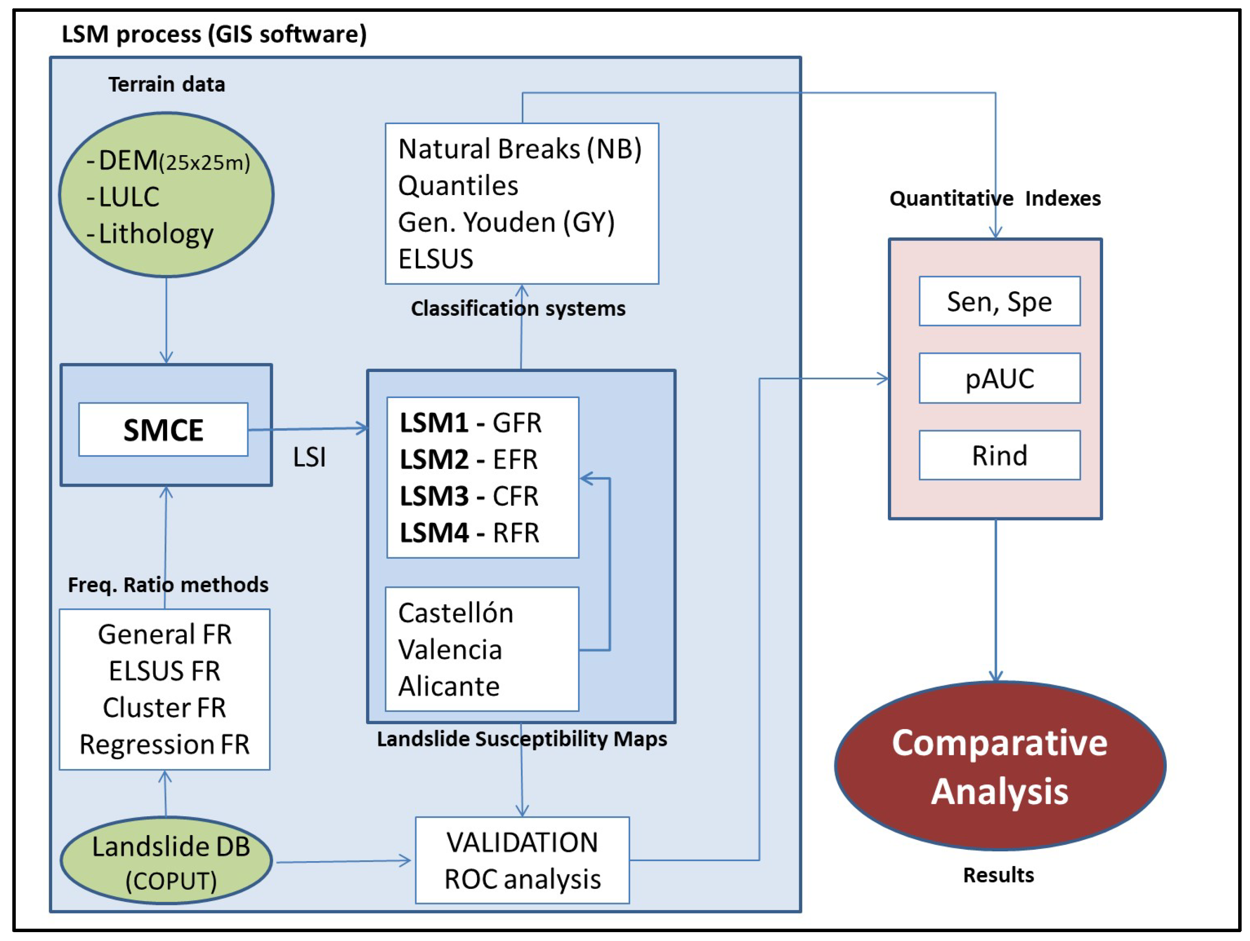
Figure 3 summarises the calculation itinerary followed until the comparative analysis was made and shows that the quantitative indices calculated for the 48 susceptibility maps obtained. For an easier understanding of the results, their means are shown for the three provinces of the working area and so, 16 means are available for each indicator. These are the previously mentioned specific Rind for the classes in the LSM. The pAUC, Sen, and Spe values obtained refer to those calculated for the lower limit of the ‘high’ class for each landslide susceptibility map. According to Table 7, this corresponds to 0.75*Sen for ELSUS and Youden’s index for GY.

4. Results

4.1. Frequency Ratio Methods

In this section, it is determined which of the FR calculation methods is the most effective. The degree of accuracy of the susceptibility maps produced is calculated, i.e., the probability that a pixel in the landslide susceptibility maps classified as unstable coincides with the areas defined in the inventory. In the tables included in this section we depict average values for the different methods and indices used to facilitate comparison among methods. According to Cantarino et al. (2019) [22], working with ROC curves is the most suitable procedure—in which the increase in sensitivity true positive rate (TPR) is plotted with the increase in false positive rate (FPR) at various threshold settings. In these curves, one of the most used indices to determine the validity of diagnostic tests is the area under the ROC curve (AUC). This is an index that shows which test best discriminates between hits and misses.

These calculations will be made on the maps of the three provinces, together with the extended inventory for the entire territory studied and all the slope values. Thus, the AUC values obtained are quite high and exceed the value of 0.841 (results shown in

Table 8. AUC values for the FR methods.

Provinces	GFR	EFR	CFR	RFR
Castellon (CST)	0.841	0.853	0.852	0.854
Valencia (VLC)	0.858	0.869	0.865	0.869
Alicante (ALC)	0.873	0.888	0.889	0.892
Mean	0.857	0.870	0.870	0.872

). The table shows that there is no significant difference when considering all the landslide susceptibility index values. Only the GFR values stand out, and these are clearly lower than the rest. This is because at low landslide susceptibility index values, the probability of landslides is low, the probability of success is high, and they represent most the pixels studied. One solution to highlight the differences would be to disregard pixels with low landslide susceptibility index values and use the cut-off points defined by one of the classifications discussed above.

However, it is preferable to establish these levels by means of ROC curves in a section of the curve that reflects the most appropriate values rather than the total set. By working on this selected range, a partial “p” AUC value (pAUC) is obtained, which is more meaningful as it does away with values that offer scarce information. Indeed, in this work, a large number of positive hits (sensitivity) is considered more important with the largest number of negative hits (specificity) in the most susceptible sections (landslide susceptibility index values). Considering the importance of specificity in landslide studies, the criterion of calculating pAUC for values greater than 60% (Spe or TNR > 0.6, or FPR < 0.4) has been adopted.

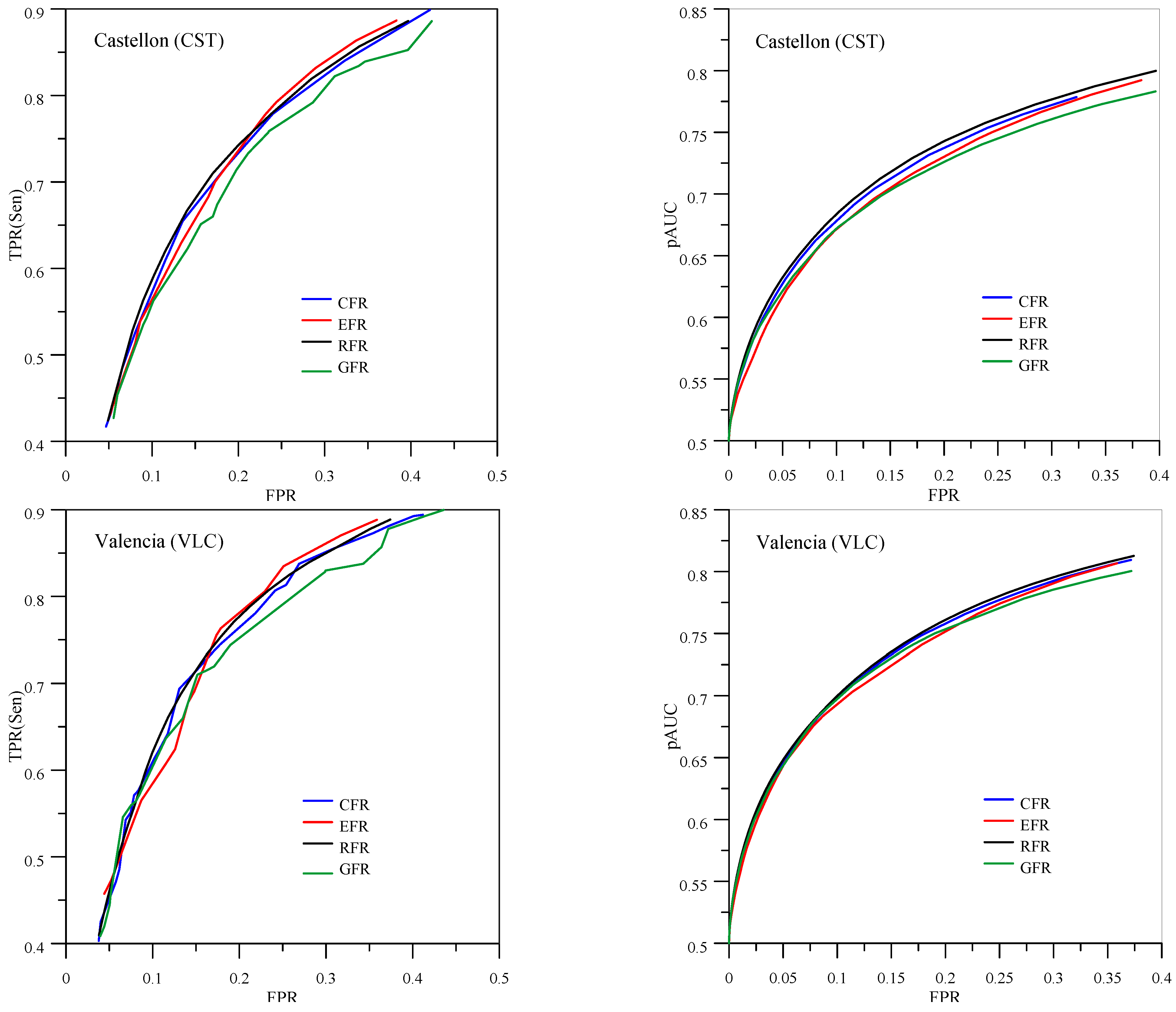
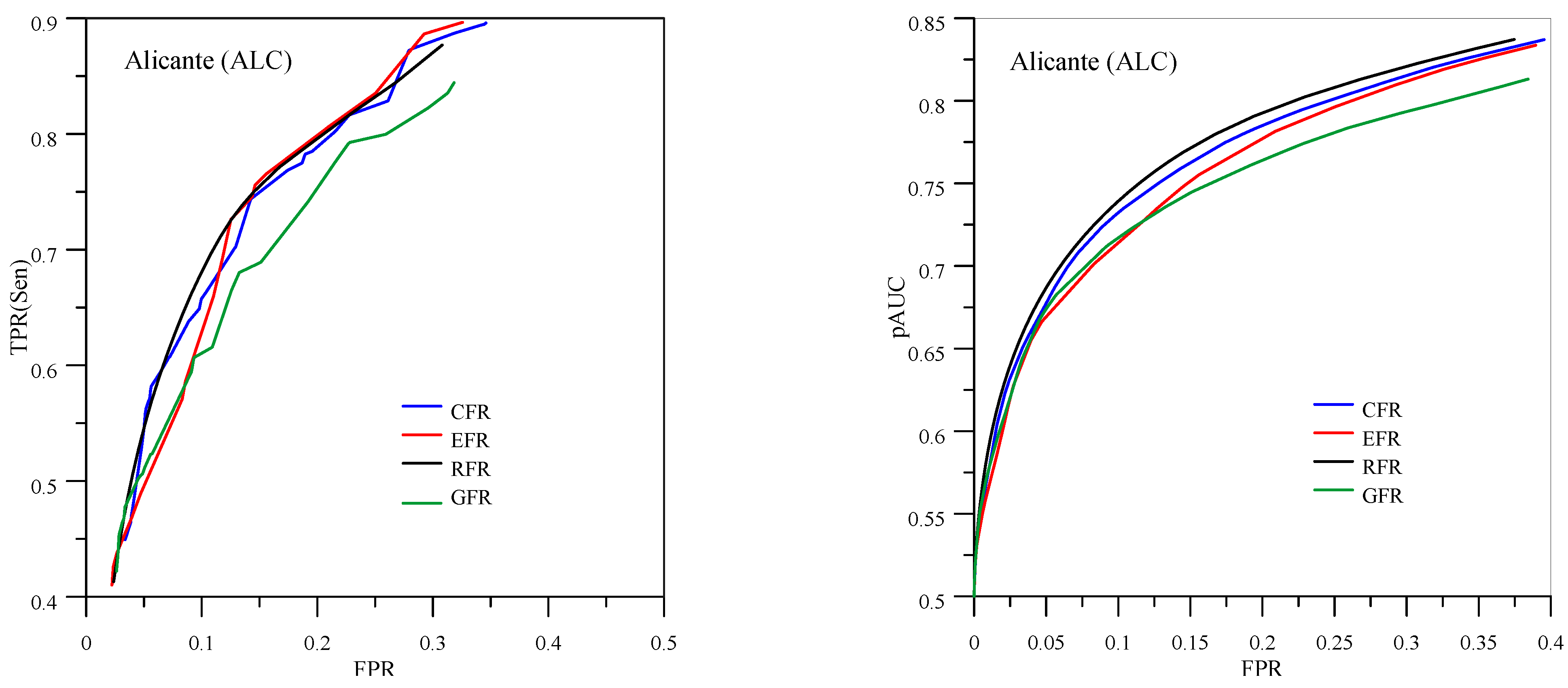
Figure 4 below explains the behaviour of the ROC curves. It shows the ROC curves for the three provinces and with high values selected on the axes for clarity: Sen > 40% and Spe > 50%. Shown alongside are the pAUC evolution plots for high specificity values (Spe > 60%) with the area between the FPR level expressed in abscissa and the beginning of the ROC curve.

According to the ROC curves in Figure 4 in areas of medium susceptibility with a hit rate for stable areas in the order of TNR = 70% (or 30% FPR), the gain in hits achieved in unstable areas (improvement in mean sensitivity) by the continuous methods (CFR and RFR) is very low (around 1–3%). With medium or low susceptibility (with TNR < 30% or FPR > 70%), no differences among methods can be seen as the curves coincide. Therefore, it does not seem worthwhile extending the zone delimited as unstable with the medium/low susceptibility zone for such a small gain (due to the increase in prevention costs that this requires). However, in the very high susceptibility zones (with TNR > 80% or FPR < 20%), the mean gain in sensitivity exceeds 5% in favour of the continuous methods (CFR and RFR).

An analysis of the evolution of pAUC for each method shown in Figure 4 is intriguing. It is conclusive to note that the continuous methods, such as CFR and especially RFR, offer a higher envelope in their pAUC values in the described range. This result guarantees the highest probability of success in the high susceptibility zone (landslide susceptibility index), and this is the desired objective.

4.2. Classification Systems

An initial approach to determine the behaviour of the classification systems shows a correlation between the landslide susceptibility index values of the treated maps. This is especially true for a comparison with ELSUS and GYouden, as their classifications are more similar. The kappa index will be used for this comparison.

Kappa is considered more robust than simply calculating the observed proportion of agreement because it accounts for the proportion of agreement that would be expected by chance. Kappa ranges from −1 to +1, with larger values indicating a higher level of concordance. It can be expressed as follows [37]:

$$\kappa =\frac{d-q}{N-q}$$

(5)

where d (observed agreement) is the proportion of cells in agreement, q is the proportion of agreement expected by chance, and N the total number of observations. The current study employed the Kappa statistic with linear weighting to measure the level of agreement between maps in all cases; see Fleiss et al. (2003) [38]. The Kappa value penalizes linear disagreement among maps on a scale from smallest to largest. This Kappa index was utilized to assess the extent of change in model classes when the FR type was varied.

Table 9. Kappa values from the comparison of RFR maps with other maps.

	RFR—G. YOUDEN			RFR—ELSUS
Provinces	GFR	EFR	CFR	GFR	EFR	CFR
Castellon (CST)	0.867	0.849	0.909	0.883	0.872	0.923
Valencia (VLC)	0.895	0.805	0.916	0.888	0.883	0.923
Alicante (ALC)	0.821	0.922	0.950	0.904	0.950	0.959
Mean	0.862	0.858	0.926	0.892	0.902	0.935

compares the models against the RFR model as a basis.

As expected, the CFR method is the most correlated with RFR. The best fit is obtained in the province of Alicante because, in the high susceptibility sections (landslide susceptibility index), the value of FR for the slope is more stable. With the GY classification, the groupings with GFR and EFR show a similar correlation with the improvement obtained with CFR being evident (0.926). In contrast, if ELSUS and RFR are used as the standard, correlations rise in most cases when compared to GY. This would seem to mean that the different groupings according to RF for ELSUS are more homogeneous and, therefore, a possible improvement in the definition of classes for the factors will have less influence.

It is Interesting to analyse the correlation values obtained using the kappa Index among the classification methods. Table 9 shows a greater homogeneity in the ELSUS system with higher values than for GY. This seems to indicate that ELSUS is worse at differentiating between the calculation methods for FR. The GY classification is less correlated and more sensitive to the differences between the FR methods.

4.3. Landslide Susceptibility Maps

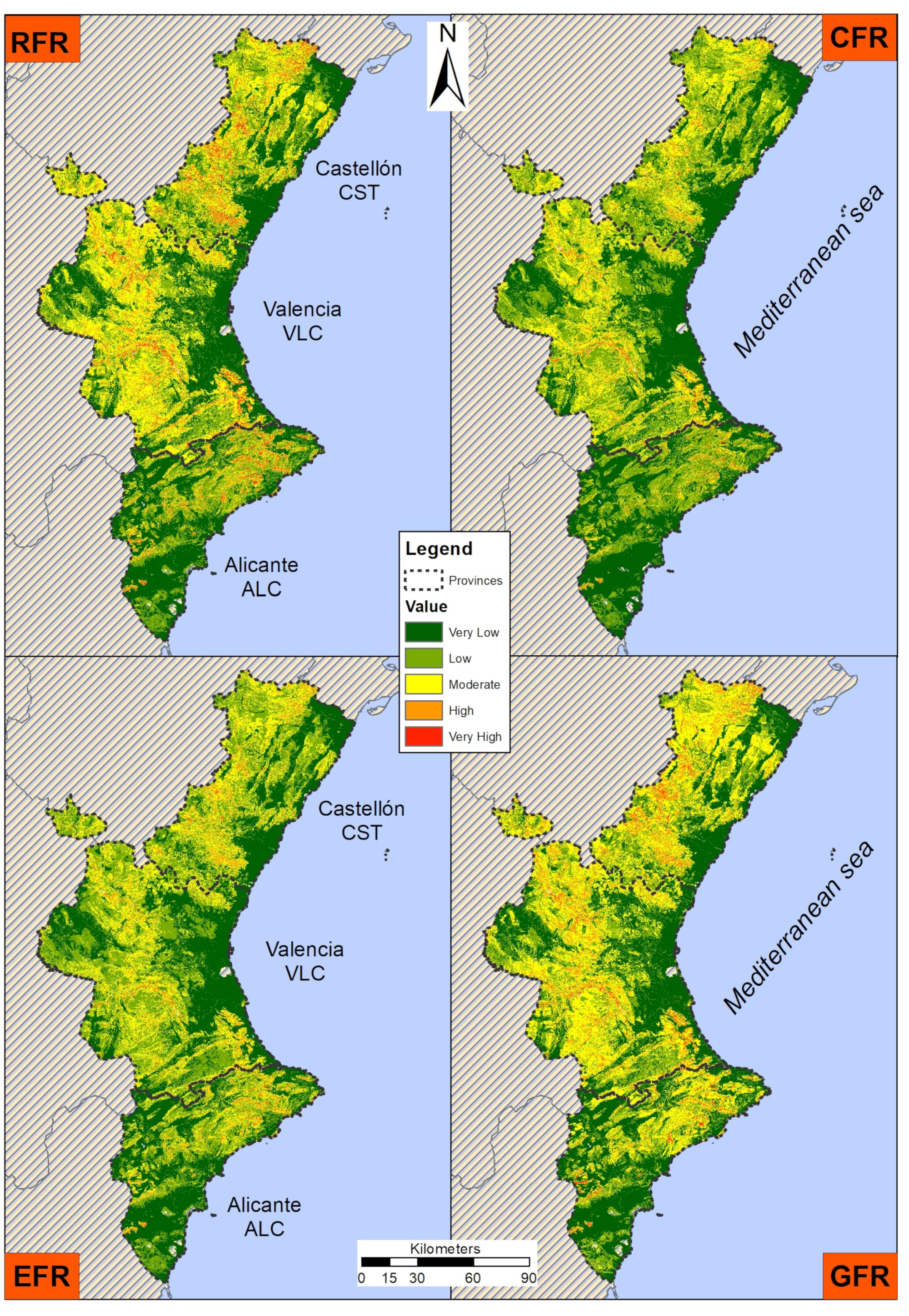
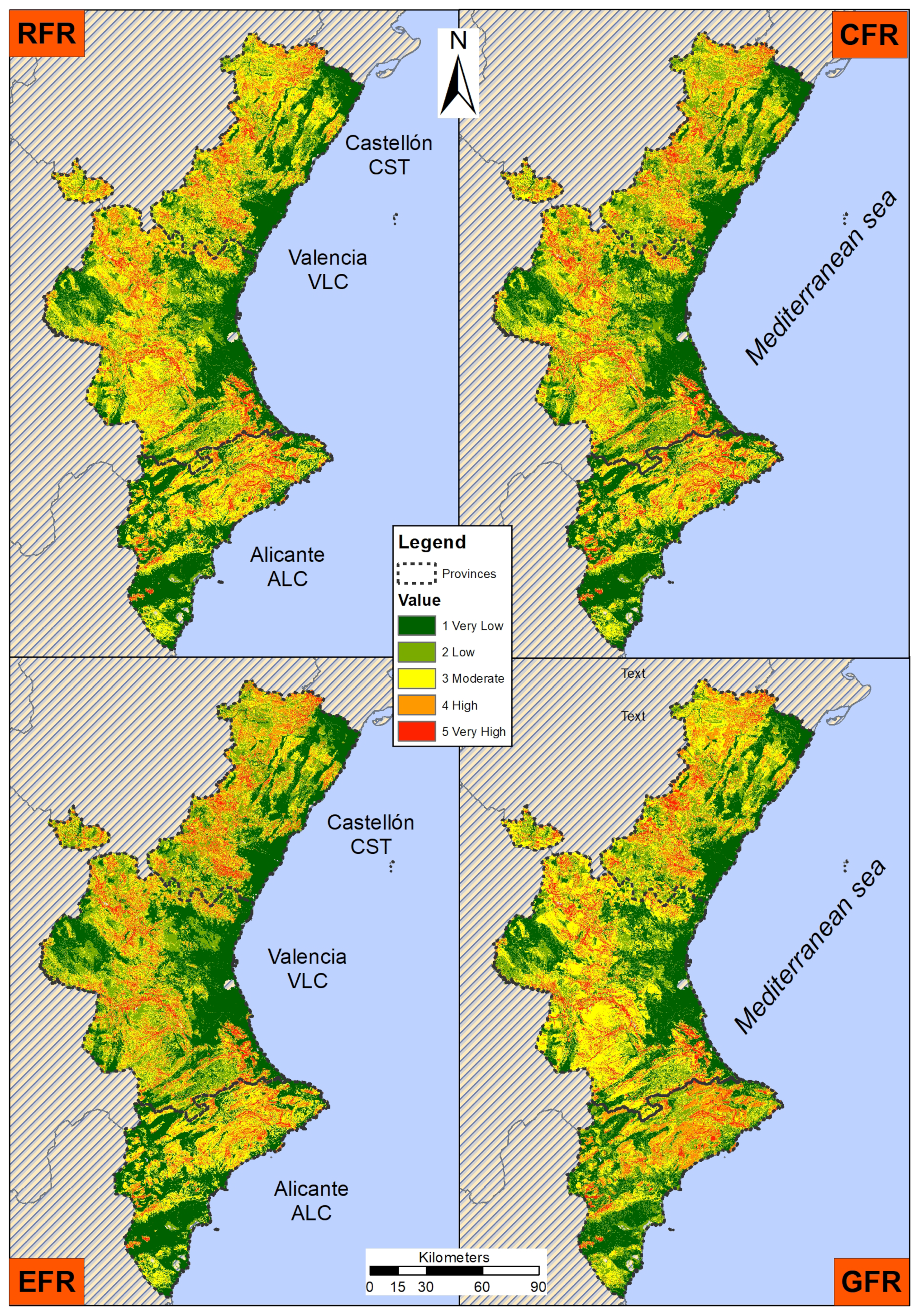
A total of 48 maps have been produced for the three provinces, the four types of FR (GFR, EFR, CFR, RFR), and the four classifications (NB, Q, ELSUS and GY). An example of these maps for the province of Valencia, prepared with regression FR (RFR) and the GY classification, is shown in Figure 5. Appendix A shows general maps for the GY and NB classifications.

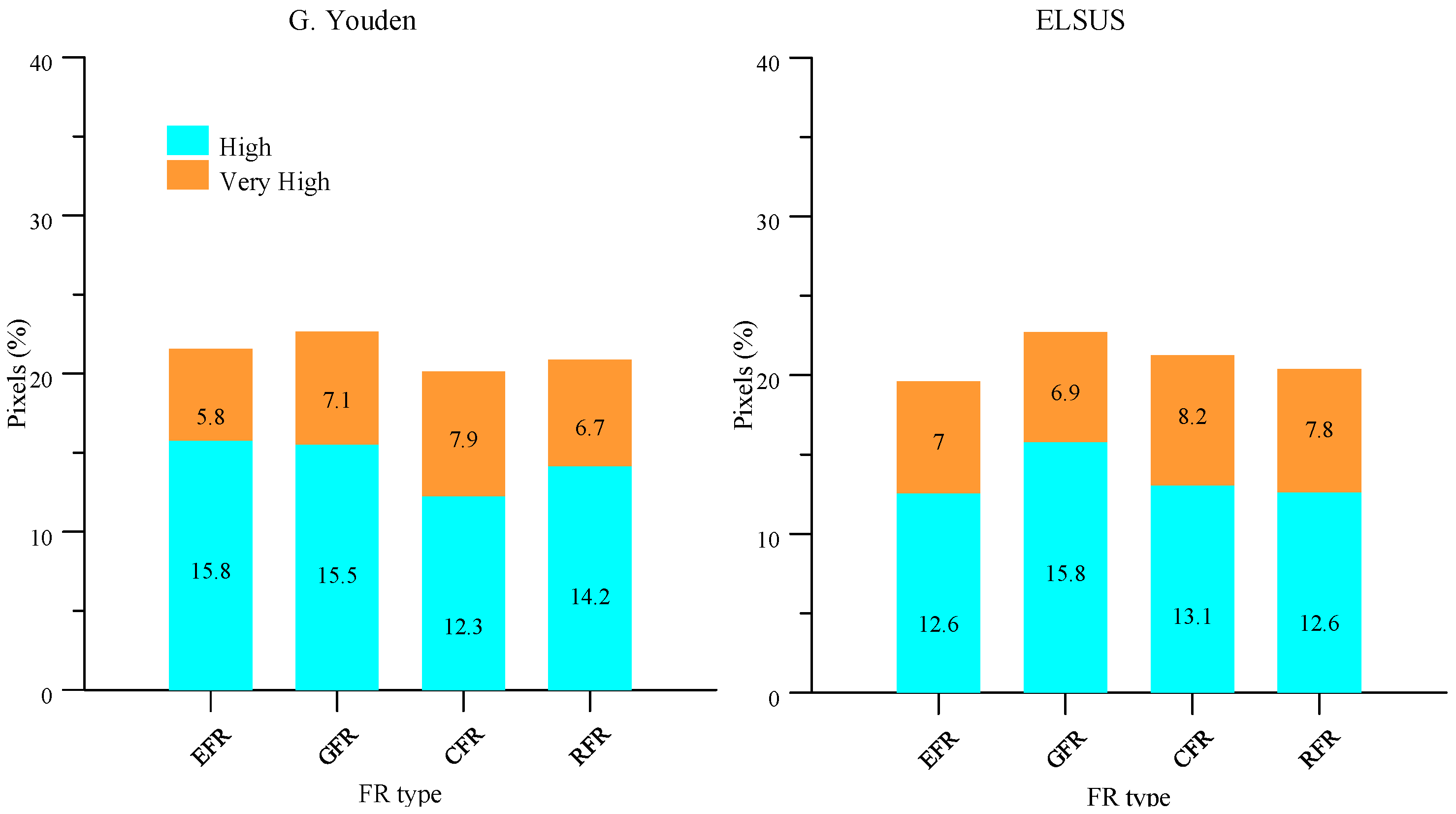
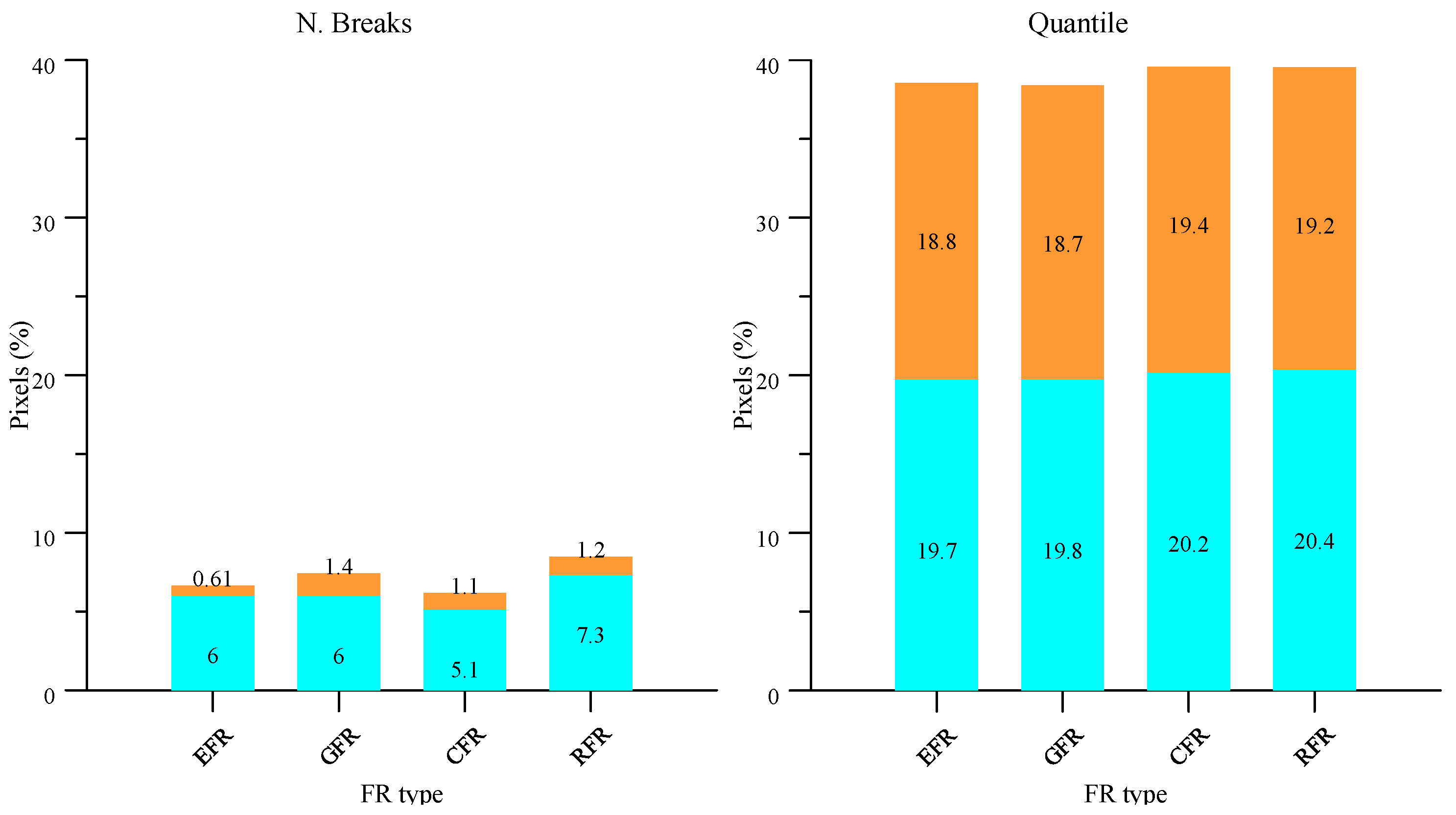
The result of the LSM classifications reveal different aspects depending on the type of FR used and above all on the classification selected. The distribution of surface areas is shown in Figure 6 for the ‘high’ and ‘very high’ susceptibility classes. This figure shows the percentage of surface area for each of these classes and for the Valencia Region as a whole (CST, VLC, and ALC).

Figure 6 clearly shows that the classification systems determine the extent of high susceptibility classes (H and VH). Natural breaks is an optimistic classification with an mean value of 15% of pixels in these classes, although it is higher for the GFR type (possibly because the division of the slope factor is better defined in the high section). On the contrary, quantiles is a pessimistic classification, with close to 40% of pixels in the high classes. The GY and ELSUS rankings seem to be more balanced in their distribution. When the different FR methods are compared, GFR shows the highest number of pixels in these classes.

4.4. Frequency Ratio and Classification Systems Comparative

Table 10. Mean values of indicators for the three provinces.

			Classification Systems
			GY	ELSUS	NBreaks	Quantil	G.Mean
Frequency ratio methods	GFR	Rind	0.771	0.717	0.789	0.761	0.759
		pAUC	0.745	0.711	0.674	0.794	0.731
		Sen	75	75	56	86	73
		Spe	80	79	91	64	79
	EFR	Rind	0.782	0.765	0.758	0.812	0.779
		pAUC	0.747	0.742	0.615	0.809	0.728
		Sen	77	75	40	89	70
		Spe	81	81	96	63	80
	CFR	Rind	0.789	0.764	0.769	0.794	0.779
		pAUC	0.761	0.755	0.597	0.823	0.734
		Sen	77	75	44	89	71
		Spe	80	82	98	62	80
	RFR	Rind	0.802	0.762	0.768	0.820	0.788
		pAUC	0.758	0.758	0.684	0.818	0.755
		Sen	80	75	56	90	75
		Spe	79	83	93	62	79
	Global mean	Rind	0.786	0.752	0.768	0.797	0.776
		pAUC	0.753	0.742	0.643	0.811	0.737
		Sen	77	75	49	89	72
		Spe	80	81	94	63	80

shows the values obtained for the indices as a mean for the three provinces. The row and column means are also included for comparisons between the FR and classification methods. In this table, the value of Sen for all cases of the ELSUS classification is 75. This is due to the very definition of its classification, which determines this value for the lower limit of the ‘high’ class (Table 2).

After applying the ELSUS classification system, no major differences are observed among FR methods, and none stands out from the others (except GFR). In the case of the GY classification, an improved overall performance is observed. In particular, the better performance of Rind seems to be due to the two lower levels that are better resolved in GY.

In terms of classification, NBreaks shows the lowest sensitivity, indicating that its hit ratio (TP) is low in high classes (H and VH). However, its failure ratio (TN) is very high. Therefore, as Figure 6 reveals, this is an excessively optimistic classification. In contrast, the quantiles classification has a high sensitivity and a very low specificity, resulting in an excessively pessimistic classification. This is the result of defining large surface areas for high susceptibilities (VH and H) with excessive false positives.

In general, GFR shows worse values than EFR, CFR, and RFR (except for the NBreaks classification). The GFR classification is very discriminating of high values, as the GFR sections are defined every 10°, which is beneficial and offers higher sensitivity than the rest. This is consistent with its higher percentage of pixels in high classes (H and VH) as shown in Figure 6. In contrast, the other FR methods have wider intervals in the high sections and show a worse fit due to their poor definition. This situation is reversed for all other and much less optimistic classifications.

LSMs based on cluster FR and regression (CFR and RFR) have better defined high LSI (landslide susceptibility index) values and show higher specificity. The ELSUS classification, based on sensitivity alone, does not satisfactorily define the best specificity results. In contrast, the GY classification improves on these results and does take specificity into account.

5. Discussion

5.1. Improvement Made by the Proposed Methods

A total of 48 susceptibility maps have been produced for three provinces by applying four types of RF and four classification systems for a large area of 23,200 km². Only 4% of this total area is considered landslide-affected, according to the COPUT inventory (1998). This fact points to the difficulty of finding clearly differentiated and generalisable results.

An analysis of Table 10 leads to the conclusion that the general method of calculating FR in constant intervals of the same amplitude (GFR) gives the worst results of all the classification types. These are predictable results, as they do not consider the singularity of the distribution of a continuous variable that explains the characteristics of the terrain—such as slope.

For a better visualisation of the results,

Table 11. Normalisation of mean values. The highest values are shaded.

	Classification Normalised Mean for All FR Types				Id. For All Classification Types
	GY	ELSUS	NBreaks	Quantil	GFR	EFR	CFR	RFR
Rind	0.76	0.00	0.36	1.00	0.16	0.61	0.60	0.81
pAUC	0.65	0.59	0.00	1.00	0.53	0.51	0.54	0.67
Sen	0.72	0.66	0.00	1.00	0.61	0.54	0.57	0.66
Spe	0.55	0.57	1.00	0.00	0.50	0.54	0.56	0.53
Mean	0.67	0.46	0.34	0.75	0.45	0.55	0.57	0.67

shows the normalised values in the interval [0,1] that correspond to the means shown in Table 10.

Table 11 shows that the GY and quantile classifications show the highest values on mean for the 42 cases analysed. It is true that quantile classification offers the highest value, clearly because it covers a much larger area of high susceptibility values and thus includes in these classes a large majority of the positive cases found. This situation results in a very low specificity and is therefore an excessively pessimistic classification because it considers 40% of the territory as highly susceptible. This does not seem acceptable, as the area affected according to the inventory is 10 times less, as mentioned above. Therefore, the quantile classification must be considered unrealistic. However, the continuous CFR methods, and especially the RFR methods, stand out on mean in all classifications used and demonstrate a better fit to the landslide inventories in almost every situation. The results are more clearly shown in Figure 7 which shows a radial plot of data from Table 11.

In addition, it is worthwhile noting that:

• The standard method of grouping classes into equal intervals (GFR) produces the worst results. Increasing the number of intervals with the same criteria does not produce an improvement.
• The ranges defined in the ELSUS methodology (EFR) produce good results. However, the criterion used is not explained in the reference article.
• The neighbourhood clustering method (CFR) is simple and offers good results that are generally better than EFR.
• The regression fit method (RFR) is somewhat complex to apply but produces the best results.

It can be confirmed with the data shown in Figure 7 that a justified improvement has been obtained with the new methods applied: CFR and GYouden. Moreover, by treating each case in three different areas (the three provinces), it can be concluded that the results achieved are sufficiently robust and generalisable.

5.2. Sensitivity and Specificity

The difference between FR types of methods (continuous or discrete) can be explained according to the objectives of the map produced. If a map is sought in which the values of greater susceptibility (landslide susceptibility index) define the unstable zones with greater accuracy (discarding zones without landslides for a better prediction for pixels without landslides, and minimising errors in the delimitation of high susceptibility zones) then the most appropriate methods are those that propose a greater density of classes in the high values of the continuous variables (CFR and RFR). However, if greater accuracy is sought for low susceptibility zones (marking the larger unstable zones for a better prediction for pixels with landslides), then conventional methods will be more appropriate even though they produce a costly excessive pessimism. The greater zoning of high slope values, when this variable is very significant in the study area, enables a better separation of unstable and stable zones, considering the varying cost of failure in the high susceptibility sections as opposed to the low susceptibility areas.

Potentially unstable sections (susceptibility classes VH and H) appear to be quite effective in defining zones with potential landslides. In particular, RFR with GY offers a high and equal sensitivity and specificity (80%). The high specificity (precision in discarding landslide areas) is very important, as false positives can lead to expensive but unnecessary slope stabilisations. Sensitivity (precision in landslide areas) is also important to prevent the occupation of potentially dangerous areas that could result in many deaths and heavy economic losses.

Finally, the ELSUS system is quite efficient with good results for all methods, but no differences can be seen. This is because it only considers sensitivity and so does not consider the improvement brought by continuous methods that also improve in specificity.

5.3. Applicability

The possibilities of application using other variables in other geographical areas are open. The application in the case study of four classification methods for the classes of the slope variable and four classification systems offer robust results that allow the proposed methods to be used without limitations. However, for the improvement in the results to be evident, the continuous variables used must have an important weight in the overall model. This methodology will be appreciated in the semi-arid climates of a large part of the Spanish territory and in other European areas (Italy, Greece, South of France, …) where the slope plays an important role.

In any case, it is important to note that while some methods work better than others, none proves superior in all conditions [1]. It is therefore very important to select, adapt and extract as much information as possible from the data and to use the experience and skill of the researchers.

6. Conclusions

In accordance with the above and considering the section on calculation methods for frequency ratio (FR), it can be concluded that establishing groupings or patterns of variation for continuous variables (the slope in this example) is worthwhile in all cases. As a result, the classes are better adjusted to the available data structure, and the subjectivity observed in many classifications of continuous factors is avoided.

When performing an ROC analysis (see Figure 4), the continuous methods offer improvements in hits (positive and negative) in the sections of the ROC curve with the greatest susceptibility to landslides. According with Thanh (2022) [39] and Xiao (2020) [32], in terms of model performance, the accuracy (by the AUC values) of the bivariate methods for landslide susceptibility mapping is approximately between 75–80% with study areas of some hundreds of square kilometers.

The current investigation offers these AUC values, but with study areas ten times larger. An improvement of 2–3% on conventional methods is achieved. In these sections, continuous methods improve specificity. This is demonstrated by looking at the ROC curve and the pAUC curves, where the improvement is up to an FPR of 0.3–0.4 and a sensitivity (positive hit) of 0.8. According to the pAUC curves, the suitability of the RFR method is assured by its appearance as the outer envelope of the other methods.

It is highly important that the regression fit method (RFR) is somewhat complex to apply but produces the best results. In the high susceptibility zone, the increase in sensitivity can be up to 10% over GFR for a given specificity. In addition, the different high susceptibility surfaces between RFR and GFR methods in the applied classification systems does not exceed 2% difference. Obviously, RFR offers a much more accurate high susceptibility surface.

The GY-based classification system, which considers sensitivity and specificity, does reveal differences in FR methods. It improves the Rind index for VH and H levels and maintains the same efficiency by covering the same surface areas at these levels. It goes without saying that any improvement brought about by the application of new calculation methods to susceptibility maps represents an increase in their effectiveness and an advance in knowledge. The results obtained in a very large study area are sufficiently solid to recommend the general use of the new proposed methodologies under similar climates.

In conclusion, the continuous methods presented in this paper for the calculation of the frequency ratio (RFR or even CFR) provide an improvement in specificity in areas of high susceptibility. In other words, areas without landslides are excluded with a higher probability of success (specificity), while maintaining a similar probability of success in locating these events (sensitivity). This is a key aspect that would avoid unnecessary costs in prevention. This improvement is transferred to susceptibility mapping much more clearly when classifications are used that incorporate sensitivity and especially, specificity parameters such as Generalised Youden.