

A Lightweight Deep Learning Model for Automatic Modulation Classification Using Residual Learning and Squeeze–Excitation Blocks


Abstract
1. Introduction
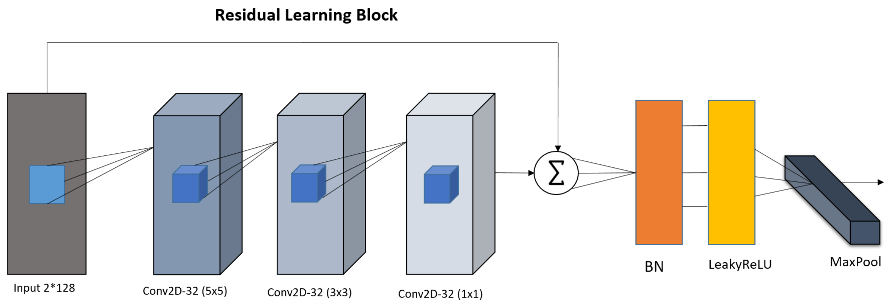
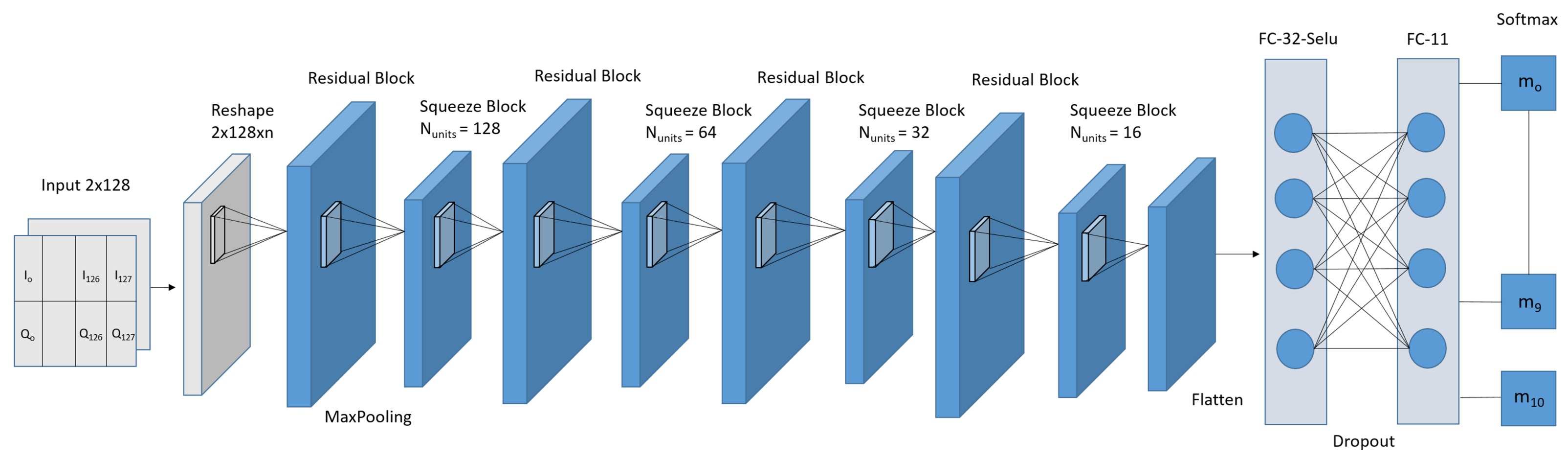
- We employed the property of a residual learning block possessing significant representational capability in order to acquire latent information from received signals repeatedly, enhancing classification accuracy.
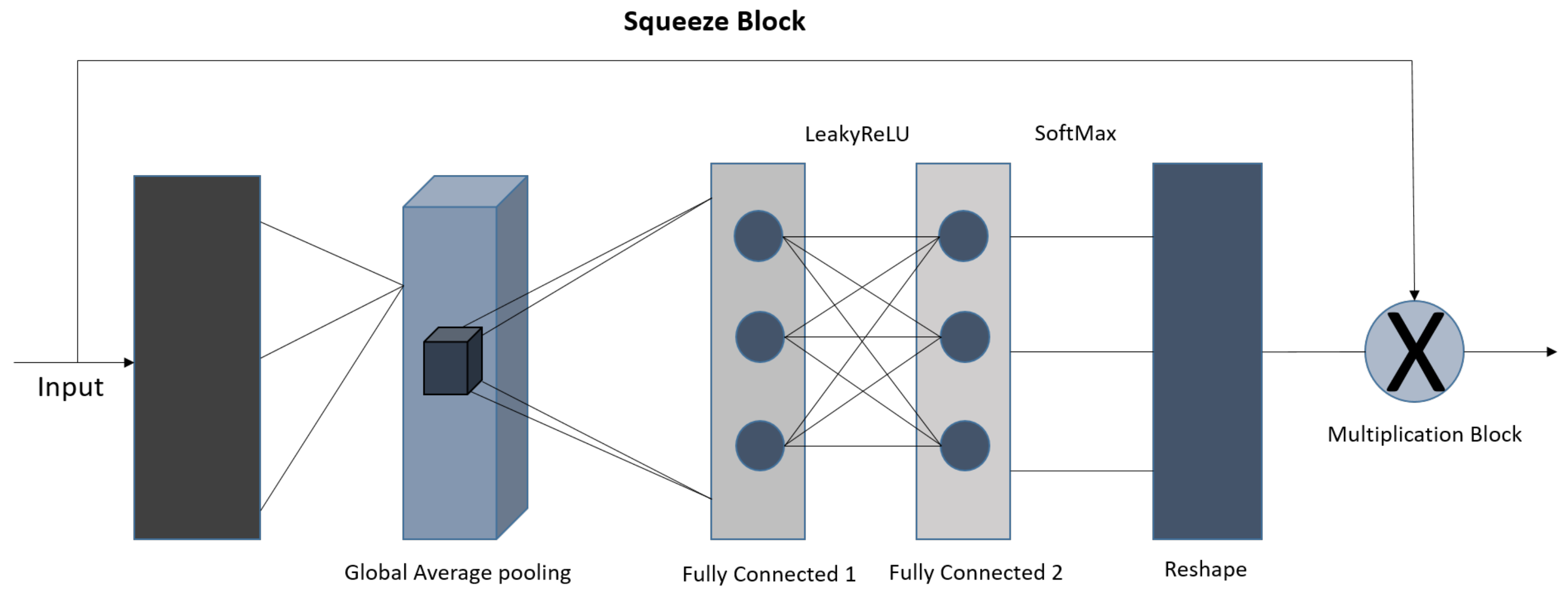
- Additionally, we utilized the squeeze-and-excitation network block that is customized for the AMC task. This takes full advantage of modeling channel interconnections and iteratively adjusts channel-wise characteristic responses to boost efficiency.
- To improve the architecture, we stacked various type of layers, such as the conv2D layer, the batch normalization layer, and the global average pooling layer, which were used to extract the features.
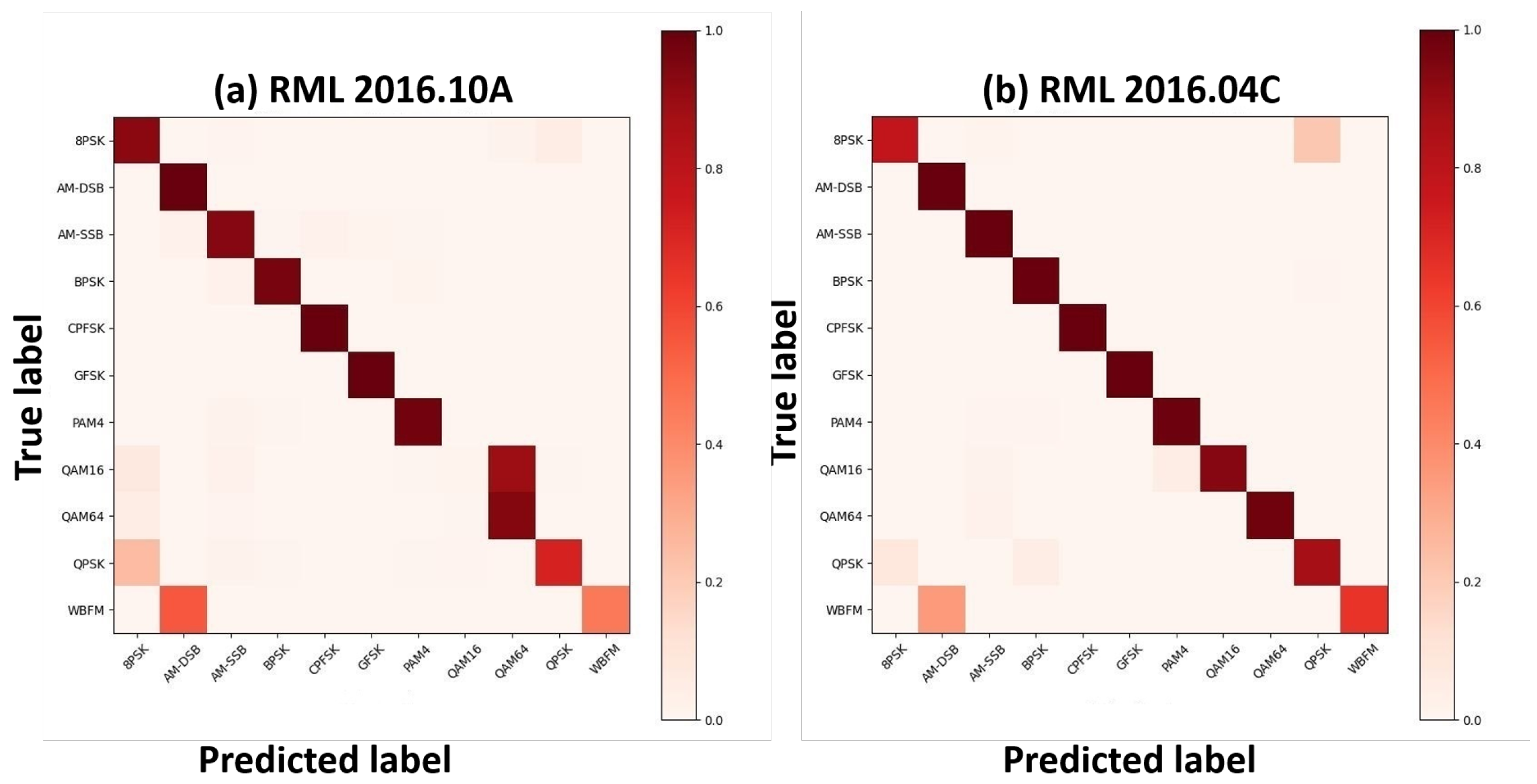
- Two datasets, namely RadioML 2016.04C and RadioML 2016.10A, were utilized from [7] to compare the effectiveness and generalization ability of AMC with diverse architecture configuration.
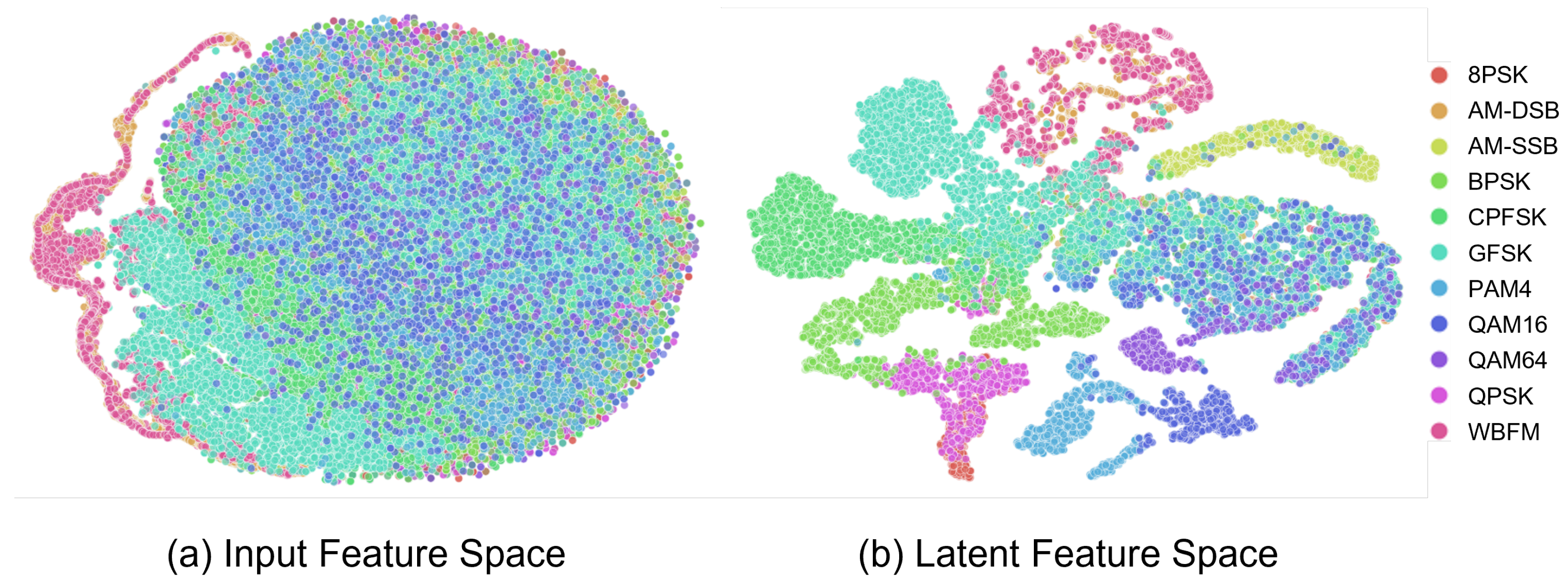
- The datasets included eleven types of modulated signals, namely QPSK, AM-DSB, AM-SSB, BPSK, CPFSK, GFSK, PAM4, QAM16, QAM64, QPSK, and WBFM. They were all utilized to train the network. The simulation results demonstrate that in terms of accuracy, by including a higher number of modulation types, the proposed model achieves better performance to extract features compared to contemporary modulation classification techniques.
2. Literature Review
2.1. Likelihood-Based (LB) Method
2.2. Feature-Based (FB) Method
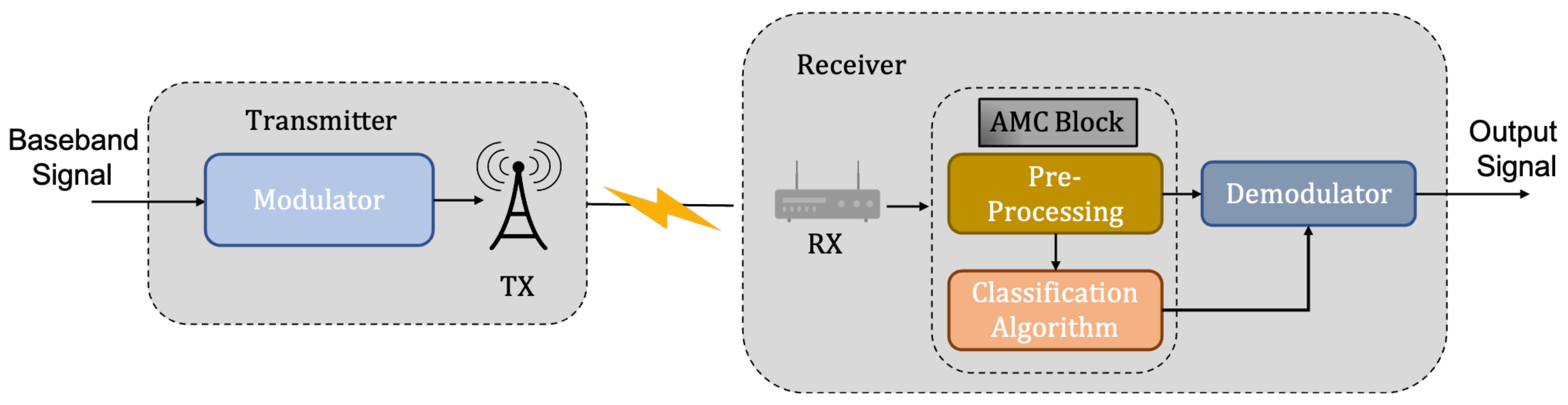
- Preprocessing: This stage is responsible for extracting features from the received signal. Different features can be chosen based on various circumstances and predictions. Certain immediate aspects of the signal, such as instantaneous signal power, frequency, phase, amplitude, and so on, are retrieved during the feature extraction phase [13]. As a result, these characteristics transform the raw data into patterns that must be learned by the classifier for the purpose of recognition.
- Classification Algorithm: The classification algorithm utilizes the features from the preprocessor as an input, and outputs the modulation type of the signal for each received signal.
Comparison between Likelihood-Based and Feature-Based Method
2.3. Deep Learning Techniques for Automatic Modulation Classification
3. Proposed Design
3.1. Residual Learning
3.2. Squeeze–Excitation Network
Overall Proposed Block
4. Results and Discussion
4.1. Dataset Description
4.2. Comparative Experiments of Various Networks
4.3. Ablation Study
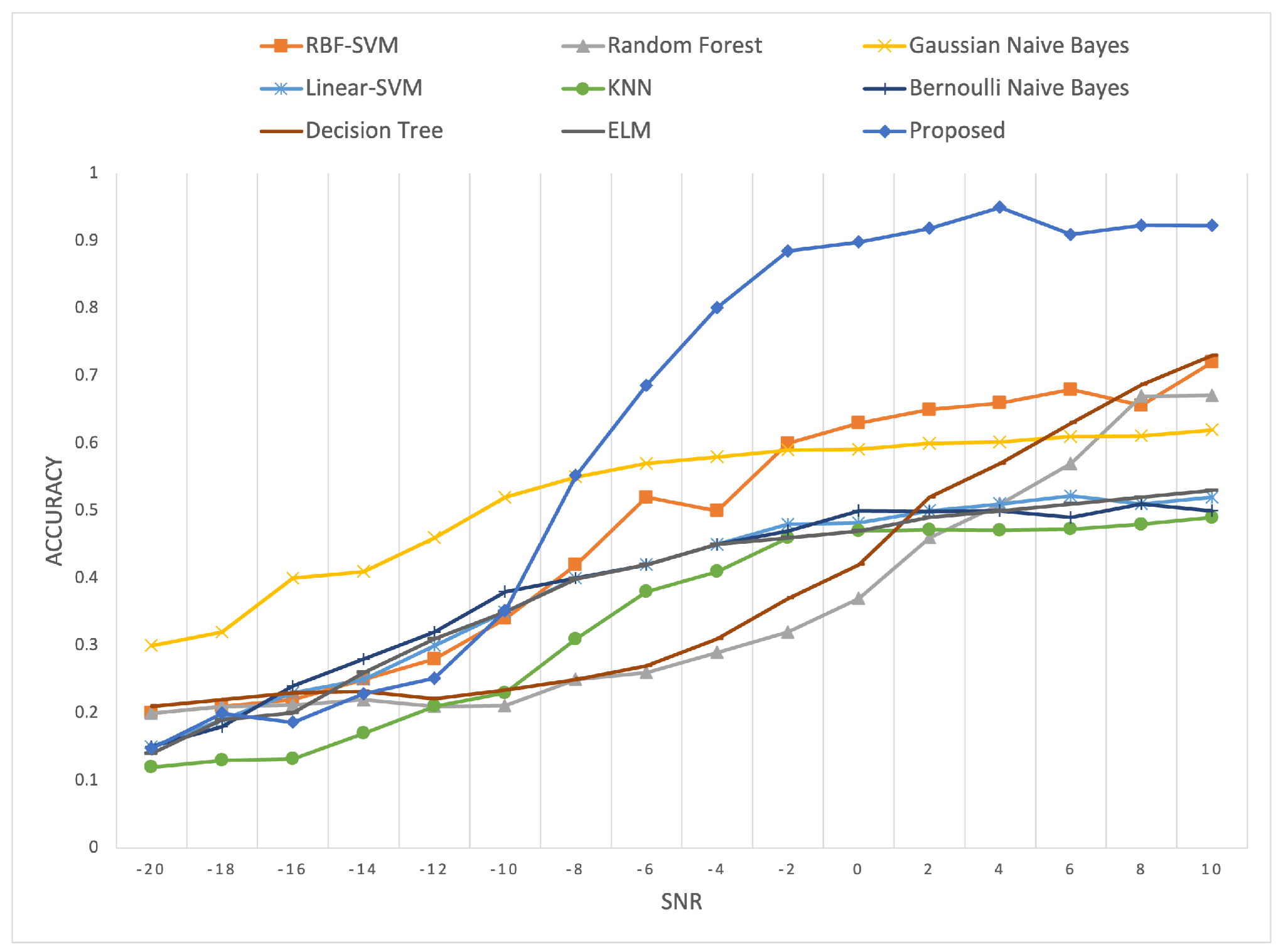
4.4. Comparison with Contemporary Methods
5. Conclusions
Author Contributions
Funding
Institutional Review Board Statement
Informed Consent Statement
Data Availability Statement
Conflicts of Interest
References
- Liu, X.; Wang, Q.; Wang, H. A Two-Fold Group Lasso Based Lightweight Deep Neural Network for Automatic Modulation Classification. In Proceedings of the 2020 IEEE International Conference on Communications Workshops (ICC Workshops), Dublin, Ireland, 7–11 June 2020; pp. 1–6. [Google Scholar] [CrossRef]
- Kim, B.; Kim, J.; Chae, H.; Yoon, D.; Choi, J.W. Deep neural network-based automatic modulation classification technique. In Proceedings of the 2016 International Conference on Information and Communication Technology Convergence (ICTC), Jeju, Republic of Korea, 19–21 October 2016; pp. 579–582. [Google Scholar]
- Liang, Y.C.; Chen, K.C.; Li, G.Y.; Mahonen, P. Cognitive radio networking and communications: An overview. IEEE Trans. Veh. Technol. 2011, 60, 3386–3407. [Google Scholar] [CrossRef]
- Triantaris, P.; Tsimbalo, E.; Chin, W.H.; Gündüz, D. Automatic modulation classification in the presence of interference. In Proceedings of the 2019 European Conference on Networks and Communications (EuCNC), Valencia, Spain, 18–21 June 2019; pp. 549–553. [Google Scholar]
- Huang, S.; Dai, R.; Huang, J.; Yao, Y.; Gao, Y.; Ning, F.; Feng, Z. Automatic modulation classification using gated recurrent residual network. IEEE Internet Things J. 2020, 7, 7795–7807. [Google Scholar] [CrossRef]
- Dobre, O.A.; Abdi, A.; Bar-Ness, Y.; Su, W. Survey of automatic modulation classification techniques: Classical approaches and new trends. IET Commun. 2007, 1, 137–156. [Google Scholar] [CrossRef]
- O’shea, T.J.; West, N. Radio machine learning dataset generation with gnu radio. In Proceedings of the 6th GNU Radio Conference, Boulder, CO, USA, 12–16 September 2016; Volume 1. [Google Scholar]
- Ramezani-Kebrya, A.; Kim, I.M.; Kim, D.I.; Chan, F.; Inkol, R. Likelihood-based modulation classification for multiple-antenna receiver. IEEE Trans. Commun. 2013, 61, 3816–3829. [Google Scholar] [CrossRef]
- Polydoros, A.; Kim, K. On the detection and classification of quadrature digital modulations in broad-band noise. IEEE Trans. Commun. 1990, 38, 1199–1211. [Google Scholar] [CrossRef]
- Panagiotou, P.; Anastasopoulos, A.; Polydoros, A. Likelihood ratio tests for modulation classification. In Proceedings of the MILCOM 2000 Proceedings. 21st Century Military Communications. Architectures and Technologies for Information Superiority (Cat. No. 00CH37155), Los Angeles, CA, USA, 22–25 October 2000; IEEE: Piscataway, NJ, USA, 2000; Volume 2, pp. 670–674. [Google Scholar]
- Majhi, S.; Gupta, R.; Xiang, W.; Glisic, S. Hierarchical hypothesis and feature-based blind modulation classification for linearly modulated signals. IEEE Trans. Veh. Technol. 2017, 66, 11057–11069. [Google Scholar] [CrossRef]
- Usman, M.; Lee, J.A. AMC-IoT: Automatic Modulation Classification Using Efficient Convolutional Neural Networks for Low Powered IoT Devices. In Proceedings of the 2020 International Conference on Information and Communication Technology Convergence (ICTC), Jeju, Republic of Korea, 21–23 October 2020; pp. 288–293. [Google Scholar]
- Ghasemzadeh, P.; Banerjee, S.; Hempel, M.; Sharif, H. Accuracy analysis of feature-based automatic modulation classification with blind modulation detection. In Proceedings of the 2019 International Conference on Computing, Networking and Communications (ICNC), Honolulu, HI, USA, 18–21 February 2019; pp. 1000–1004. [Google Scholar]
- Khan, R.; Yang, Q.; Ullah, I.; Rehman, A.U.; Tufail, A.B.; Noor, A.; Rehman, A.; Cengiz, K. 3D convolutional neural networks based automatic modulation classification in the presence of channel noise. IET Commun. 2022, 16, 497–509. [Google Scholar] [CrossRef]
- Huang, S.; Yao, Y.; Wei, Z.; Feng, Z.; Zhang, P. Automatic modulation classification of overlapped sources using multiple cumulants. IEEE Trans. Veh. Technol. 2016, 66, 6089–6101. [Google Scholar] [CrossRef]
- Ho, K.; Prokopiw, W.; Chan, Y. Modulation identification of digital signals by the wavelet transform. IEE Proc.-Radar, Sonar Navig. 2000, 147, 169–176. [Google Scholar] [CrossRef]
- Dobre, O.A.; Oner, M.; Rajan, S.; Inkol, R. Cyclostationarity-based robust algorithms for QAM signal identification. IEEE Commun. Lett. 2011, 16, 12–15. [Google Scholar] [CrossRef]
- Huynh-The, T.; Nguyen, T.V.; Pham, Q.V.; Kim, D.S.; Da Costa, D.B. MIMO-OFDM Modulation Classification Using Three-Dimensional Convolutional Network. IEEE Trans. Veh. Technol. 2022, 71, 6738–6743. [Google Scholar] [CrossRef]
- Cardoso, C.; Castro, A.R.; Klautau, A. An efficient FPGA IP core for automatic modulation classification. IEEE Embed. Syst. Lett. 2013, 5, 42–45. [Google Scholar] [CrossRef]
- Hou, C.; Liu, G.; Tian, Q.; Zhou, Z.; Hua, L.; Lin, Y. Multi-signal Modulation Classification Using Sliding Window Detection and Complex Convolutional Network in Frequency Domain. IEEE Internet Things J. 2022, 9, 19438–19449. [Google Scholar] [CrossRef]
- Hazza, A.; Shoaib, M.; Alshebeili, S.A.; Fahad, A. An overview of feature-based methods for digital modulation classification. In Proceedings of the 2013 1st International Conference on Communications, Signal Processing, and Their Applications (ICCSPA), Sharjah, United Arab Emirates, 12–14 February 2013; pp. 1–6. [Google Scholar]
- Hameed, F.; Dobre, O.A.; Popescu, D.C. On the likelihood-based approach to modulation classification. IEEE Trans. Wirel. Commun. 2009, 8, 5884–5892. [Google Scholar] [CrossRef]
- Abdel-Moneim, M.A.; Al-Makhlasawy, R.M.; Abdel-Salam Bauomy, N.; El-Rabaie, E.S.M.; El-Shafai, W.; Farghal, A.E.; Abd El-Samie, F.E. An efficient modulation classification method using signal constellation diagrams with convolutional neural networks, Gabor filtering, and thresholding. Trans. Emerg. Telecommun. Technol. 2022, 33, e4459. [Google Scholar] [CrossRef]
- Zhou, Y.; Fadlullah, Z.M.; Mao, B.; Kato, N. A deep-learning-based radio resource assignment technique for 5G ultra dense networks. IEEE Netw. 2018, 32, 28–34. [Google Scholar] [CrossRef]
- Huang, H.; Guo, S.; Gui, G.; Yang, Z.; Zhang, J.; Sari, H.; Adachi, F. Deep learning for physical-layer 5G wireless techniques: Opportunities, challenges and solutions. IEEE Wirel. Commun. 2019, 27, 214–222. [Google Scholar] [CrossRef]
- Farhad, A.; Kim, D.H.; Yoon, J.S.; Pyun, J.Y. Deep Learning-Based Channel Adaptive Resource Allocation in LoRaWAN. In Proceedings of the 2022 International Conference on Electronics, Information, and Communication (ICEIC), Jeju, Republic of Korea, 6–9 February 2022; pp. 1–5. [Google Scholar]
- Blanco-Filgueira, B.; Garcia-Lesta, D.; Fernández-Sanjurjo, M.; Brea, V.M.; López, P. Deep learning-based multiple object visual tracking on embedded system for IoT and mobile edge computing applications. IEEE Internet Things J. 2019, 6, 5423–5431. [Google Scholar] [CrossRef]
- Usama, M.; Lee, I.Y. Data-Driven Non-Linear Current Controller Based on Deep Symbolic Regression for SPMSM. Sensors 2022, 22, 8240. [Google Scholar] [CrossRef]
- Deng, L.; Hinton, G.; Kingsbury, B. New types of deep neural network learning for speech recognition and related applications: An overview. In Proceedings of the 2013 IEEE International Conference on Acoustics, Speech and Signal Processing, Vancouver, BC, Canada, 26–31 May 2013; pp. 8599–8603. [Google Scholar]
- Usman, M.; Khan, S.; Lee, J.A. Afp-lse: Antifreeze proteins prediction using latent space encoding of composition of k-spaced amino acid pairs. Sci. Rep. 2020, 10, 7197. [Google Scholar] [CrossRef]
- Usman, M.; Khan, S.; Park, S.; Lee, J.A. AoP-LSE: Antioxidant Proteins Classification Using Deep Latent Space Encoding of Sequence Features. Curr. Issues Mol. Biol. 2021, 43, 1489–1501. [Google Scholar] [CrossRef] [PubMed]
- Wei, X.; Luo, W.; Zhang, X.; Yang, J.; Gui, G.; Ohtsuki, T. Differentiable Architecture Search-Based Automatic Modulation Classification. In Proceedings of the 2021 IEEE Wireless Communications and Networking Conference (WCNC), Nanjing, China, 29 March–1 April 2021; pp. 1–6. [Google Scholar]
- Ullah, A.; Abbas, Z.H.; Zaib, A.; Ullah, I.; Muhammad, F.; Idrees, M.; Khattak, S. Likelihood ascent search augmented sphere decoding receiver for MIMO systems using M-QAM constellations. IET Commun. 2020, 14, 4152–4158. [Google Scholar] [CrossRef]
- Guo, Y.; Liu, Y.; Oerlemans, A.; Lao, S.; Wu, S.; Lew, M.S. Deep learning for visual understanding: A review. Neurocomputing 2016, 187, 27–48. [Google Scholar] [CrossRef]
- O’Shea, T.J.; Corgan, J.; Clancy, T.C. Convolutional radio modulation recognition networks. In International Conference on Engineering Applications of Neural Networks; Springer: Cham, Switzerland, 2016; pp. 213–226. [Google Scholar]
- Yashashwi, K.; Sethi, A.; Chaporkar, P. A learnable distortion correction module for modulation recognition. IEEE Wirel. Commun. Lett. 2018, 8, 77–80. [Google Scholar] [CrossRef]
- He, K.; Zhang, X.; Ren, S.; Sun, J. Deep residual learning for image recognition. In Proceedings of the IEEE Conference on Computer Vision and Pattern Recognition, Las Vegas, NV, USA, 27–30 June 2016; pp. 770–778. [Google Scholar]
- Liu, X.; Yang, D.; El Gamal, A. Deep neural network architectures for modulation classification. In Proceedings of the 2017 51st Asilomar Conference on Signals, Systems, and Computers, Pacific Grove, CA, USA, 29 October–1 November 2017; pp. 915–919. [Google Scholar]
- Yao, T.; Chai, Y.; Wang, S.; Miao, X.; Bu, X. Radio signal automatic modulation classification based on deep learning and expert features. In Proceedings of the 2020 IEEE 4th Information Technology, Networking, Electronic and Automation Control Conference (ITNEC), Chongqing, China, 12–14 June 2020; Volume 1, pp. 1225–1230. [Google Scholar]
- Zhang, H.; Huang, M.; Yang, J.; Sun, W. A Data Preprocessing Method for Automatic Modulation Classification Based on CNN. IEEE Commun. Lett. 2020, 25, 1206–1210. [Google Scholar] [CrossRef]
- Ramjee, S.; Ju, S.; Yang, D.; Liu, X.; Gamal, A.E.; Eldar, Y.C. Fast deep learning for automatic modulation classification. arXiv 2019, arXiv:1901.05850. [Google Scholar]
- Miao, J.; Xu, S.; Zou, B.; Qiao, Y. ResNet based on feature-inspired gating strategy. Multimed. Tools Appl. 2022, 81, 19283–19300. [Google Scholar] [CrossRef]
- Li, W.; Guo, Y.; Wang, B.; Yang, B. Learning spatiotemporal embedding with gated convolutional recurrent networks for translation initiation site prediction. Pattern Recognit. 2023, 136, 109234. [Google Scholar] [CrossRef]
- Subramanian, M.; Shanmugavadivel, K.; Nandhini, P. On fine-tuning deep learning models using transfer learning and hyper-parameters optimization for disease identification in maize leaves. Neural Comput. Appl. 2022, 34, 13951–13968. [Google Scholar] [CrossRef]
- Xuan, H.; Liu, J.; Yang, P.; Gu, G.; Cui, D. Emotion Recognition from EEG Using All-Convolution Residual Neural Network. In International Workshop on Human Brain and Artificial Intelligence; Springer: Singapore, 2023; pp. 73–85. [Google Scholar]
- Ioffe, S.; Szegedy, C. Batch normalization: Accelerating deep network training by reducing internal covariate shift. In Proceedings of the International Conference on Machine Learning, Lille, France, 7–9 July 2015; pp. 448–456. [Google Scholar]
- Hu, J.; Shen, L.; Sun, G. Squeeze-and-excitation networks. In Proceedings of the IEEE Conference on Computer Vision and Pattern Recognition, Salt Lake City, UT, USA, 18–22 June 2018; pp. 7132–7141. [Google Scholar]
- Glorot, X.; Bengio, Y. Understanding the difficulty of training deep feedforward neural networks. In Proceedings of the Thirteenth International Conference on Artificial Intelligence and Statistics, Sardinia, Italy, 13–15 May 2010; JMLR Workshop and Conference Proceedings. pp. 249–256. [Google Scholar]
- Goodfellow, I.; Bengio, Y.; Courville, A. Deep Learning; MIT Press: Cambridge, MA, USA, 2016. [Google Scholar]
- Hong, D.; Zhang, Z.; Xu, X. Automatic modulation classification using recurrent neural networks. In Proceedings of the 2017 3rd IEEE International Conference on Computer and Communications (ICCC), Chengdu, China, 13–16 December 2017; pp. 695–700. [Google Scholar]
- West, N.E.; O’shea, T. Deep architectures for modulation recognition. In Proceedings of the 2017 IEEE International Symposium on Dynamic Spectrum Access Networks (DySPAN), Baltimore, MD, USA, 6–9 March 2017; pp. 1–6. [Google Scholar]
- Jagannath, J.; Polosky, N.; O’Connor, D.; Theagarajan, L.N.; Sheaffer, B.; Foulke, S.; Varshney, P.K. Artificial neural network based automatic modulation classification over a software defined radio testbed. In Proceedings of the 2018 IEEE International Conference on Communications (ICC), Kansas City, MO, USA, 20–24 May 2018; pp. 1–6. [Google Scholar]
- O’Shea, T.J.; Roy, T.; Clancy, T.C. Over-the-air deep learning based radio signal classification. IEEE J. Sel. Top. Signal Process. 2018, 12, 168–179. [Google Scholar] [CrossRef]
- Zhang, Z.; Tu, Y. A Pruning Neural Network for Automatic Modulation Classification. In Proceedings of the 2021 8th International Conference on Dependable Systems and Their Applications (DSA), Yinchuan, China, 5–6 August 2021; pp. 189–194. [Google Scholar]
- Güner, A.; Alçin, Ö.F.; Şengür, A. Automatic digital modulation classification using extreme learning machine with local binary pattern histogram features. Measurement 2019, 145, 214–225. [Google Scholar] [CrossRef]
- Rajendran, S.; Meert, W.; Giustiniano, D.; Lenders, V.; Pollin, S. Deep learning models for wireless signal classification with distributed low-cost spectrum sensors. IEEE Trans. Cogn. Commun. Netw. 2018, 4, 433–445. [Google Scholar] [CrossRef]
- Dai, H.; Chembo, Y.K. Classification of IQ-modulated signals based on reservoir computing with narrowband optoelectronic oscillators. IEEE J. Quantum Electron. 2021, 57, 5000408. [Google Scholar] [CrossRef]
- Wang, Y.; Liu, M.; Yang, J.; Gui, G. Data-driven deep learning for automatic modulation recognition in cognitive radios. IEEE Trans. Veh. Technol. 2019, 68, 4074–4077. [Google Scholar] [CrossRef]
- Cyclostationary Signal Processing. Available online: https://www.cyclostationary.blog (accessed on 5 April 2023).
- Jiao, J.; Sun, X.; Zhang, Y.; Liu, L.; Shao, J.; Lyu, J.; Fang, L. Modulation recognition of radio signals based on edge computing and convolutional neural network. J. Commun. Inf. Netw. 2021, 6, 280–300. [Google Scholar] [CrossRef]
- Xu, J.; Luo, C.; Parr, G.; Luo, Y. A spatiotemporal multi-channel learning framework for automatic modulation recognition. IEEE Wirel. Commun. Lett. 2020, 9, 1629–1632. [Google Scholar] [CrossRef]
- Alzaq-Osmanoglu, H.; Alrehaili, J.; Ustundag, B.B. Low-SNR Modulation Recognition based on Deep Learning on Software Defined Radio. In Proceedings of the 2022 5th International Conference on Advanced Communication Technologies and Networking (CommNet), Marrakech, Morocco, 12–14 December 2022; pp. 1–6. [Google Scholar]
- Dong, B.; Liu, Y.; Gui, G.; Fu, X.; Dong, H.; Adebisi, B.; Gacanin, H.; Sari, H. A Lightweight Decentralized-Learning-Based Automatic Modulation Classification Method for Resource-Constrained Edge Devices. IEEE Internet Things J. 2022, 9, 24708–24720. [Google Scholar] [CrossRef]
- Wang, N.; Liu, Y.; Ma, L.; Yang, Y.; Wang, H. Multidimensional CNN-LSTM network for automatic modulation classification. Electronics 2021, 10, 1649. [Google Scholar] [CrossRef]


| Classes | BPSK, AM-DSB, AM-SSB, 8PSK, QPSK, BFSK, CPFSK, QAM16, QAM64, PAM4, WB-FM |
| Sample length | 128 |
| SNR Range | −20 dB to 18 dB |
| Databases | RadioML 2016.04C, RadioML 2016.10A |
| Number of Samples | 162,060, 220,000 |
| Architecture | Parameters | Reduction | FLOPs |
|---|---|---|---|
| Inception [51] | 23.9 M | – | 1502 M |
| GRU2 [50] | 4.8 M | 0.234 M | |
| ResNet [53] | 2.7 M | 149 M | |
| CLDNN [50] | 2.6 M | 1.65 M | |
| Conv2D [12] | 921,611 | 3.15 M | |
| 2DCNN [35] | 900,000 | 29.6 K | |
| ANN [52] | 670,000 | NA | |
| Depthwise [12] | 596,491 | 3.58 M | |
| Separable [12] | 385,307 | 18.6 M | |
| Pruned CNN [54] | 36.6 M | NA | 116.6 M |
| Proposed | 253,274 | 748.88 M |
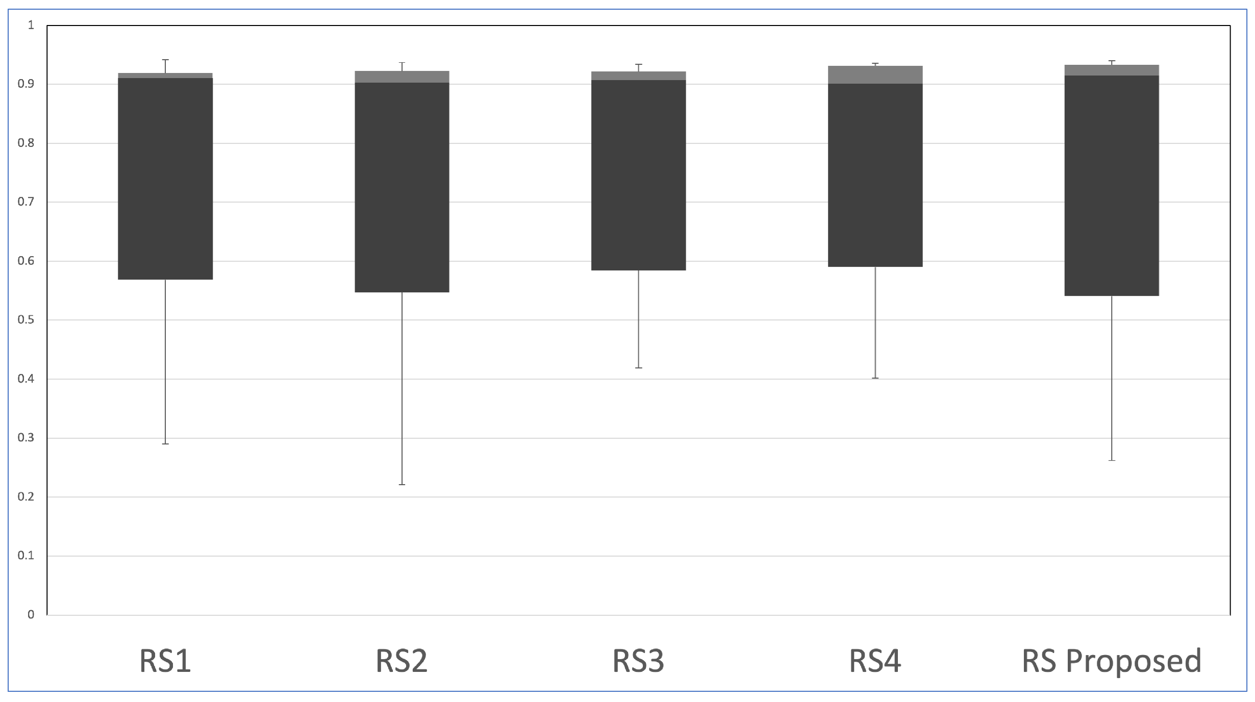
| Models | Network Structure |
|---|---|
| RS-1 | RS, RS, RS, FC |
| RS-2 | RS, RS, RS, RS, RS, RS, FC, FC |
| RS-3 | RS, RS, RS, RS, RS, FC, FC, kernel size and filter replaced |
| RS-4 | RS, global average pooling 2D, RS, RS, RS, FC, FC |
| RS-Proposed | RS, RS, RS, RS, max pooling 2D, FC, FC |
| Neural Network | Parameters | Model Weight | Accuracy |
|---|---|---|---|
| RS-1 | 265,929 | 1.1 MB | % |
| RS-2 | 256,354 | 980 Kb | % |
| RS-3 | 283,142 | 1.668 MB | % |
| RS-4 | 259,258 | 1.52 MB | % |
| RS-Proposed | 253,274 | 920 KB | % |
| Paper | Dataset | Accuracy Per SNR | Classification Method | Architecture |
|---|---|---|---|---|
| [7] | Radio ML2016.04C | 91.91% for SNR = 18 dB, Range [−20, +18] | Feature-Based | VTCNN2 |
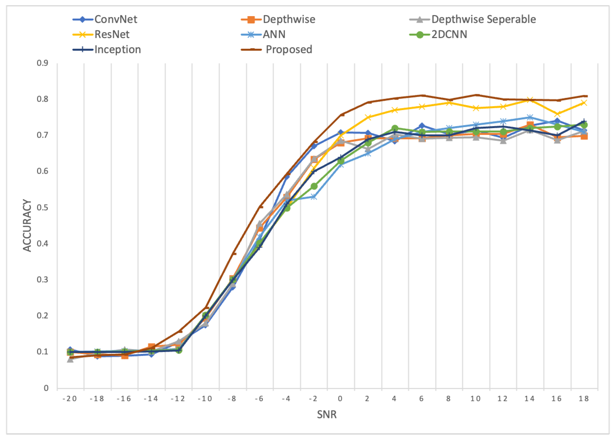
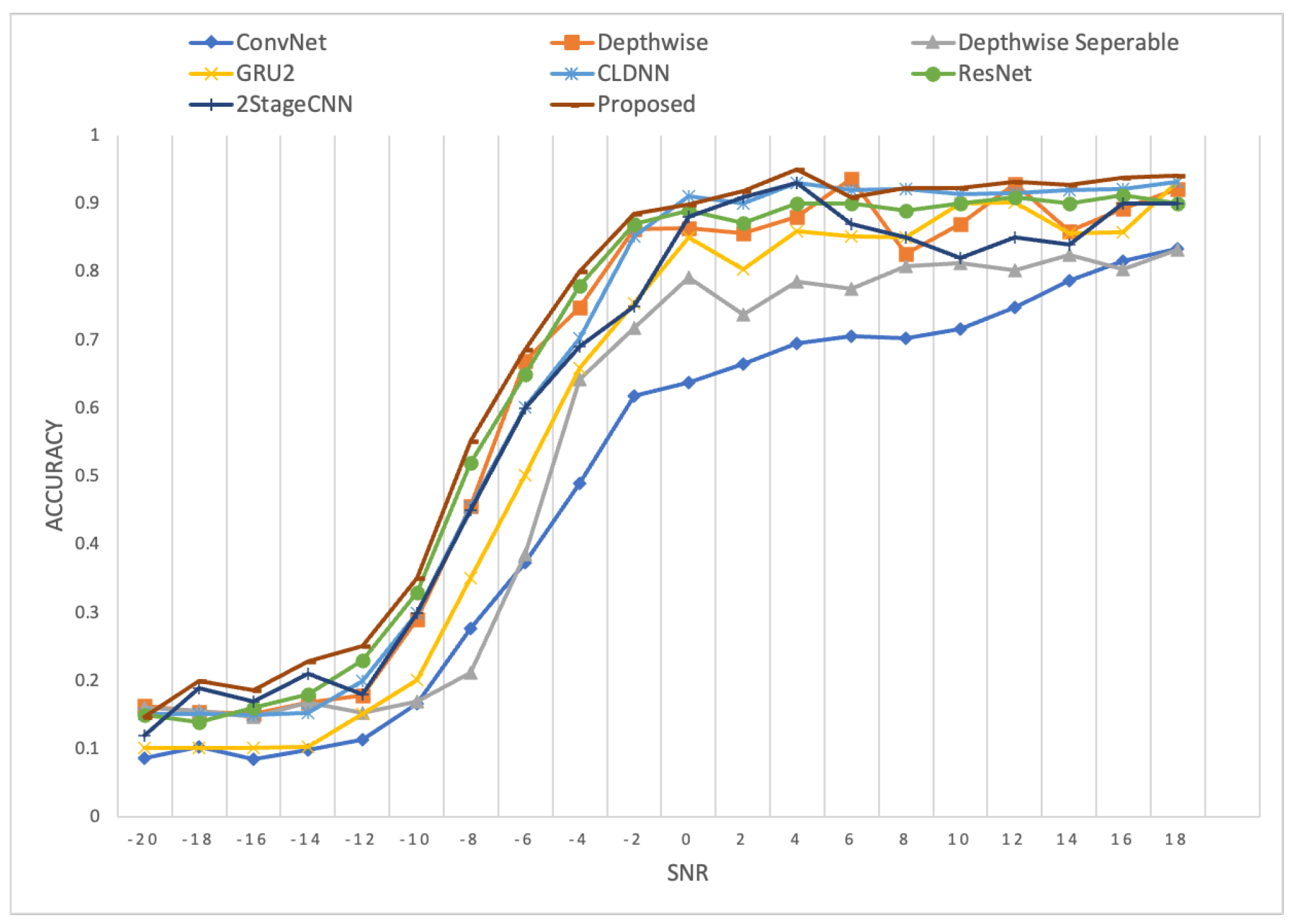
| [12] | = RML2016.10A, = RML2016.04C | 69.90% for SNR = 18 dB for , and 92.10% at SNR = 18 dB for , Range [−20, +18] | Feature-Based | Depthwise |
| [12] | = RML2016.10A, = RML2016.04C | 71.30% for SNR= 18 dB for , and 83.4% at SNR = 18 dB for , Range [−20, +18] | Feature-Based | Conv2D |
| [12] | = RML2016.10A, = RML2016.04C | 71.25% for SNR = 18 dB for , and 83.03% at SNR = 18 dB for , Range [−20, +18] | Feature-Based | Separable |
| [35] | = RML2016.10A, = RML2016.04C | 73% for SNR = 18 dB for , and 87.4% at SNR = 18 dB for , Range [−20, +18] | Feature-Based | 2DCNN |
| [36] | RadioML2016.10A | 80% for SNR > 0 dB, Range [−20, +18] | Feature-Based | CM+CNN |
| [57] | RadioML2016.04C | 88.94% for SNR =18 dB, Range [−20, +18] | Feature-Based | RCN |
| [53] | = RML2016.10A, = RML2016.04C | 79% for SNR = 18 dB for , and 90% at SNR = 18 dB for , Range [−20, +18] | Feature-Based | ResNet |
| [52] | RadioML2016.10.A | 71% for SNR = 18 dB, Range [−20, +18] | Feature-Based | ANN |
| [51] | RadioML2016.10.A | 74% for SNR = 18 dB, Range [−20, +18] | Feature-Based | Inception |
| [50] | RadioML2016.04C | 93.20% for SNR = 18 dB, Range [−20, +18] | Feature-Based | GRU2 |
| [50] | RadioML2016.04C | 93.22% for SNR = 18 dB, Range [−20, +18] | Feature-Based | CLDNN |
| [58] | RadioML2016.04C | 90% for SNR = 18 dB, Range [−20, +18] | Feature-Based | CNN |
| Proposed | = RML2016.10A, = RML2016.04C | 81.0% for SNR = 18 dB for , and 94.05% at SNR = 18 dB for , Range [−20, +18] | Feature-Based | Residual+SE |
Disclaimer/Publisher’s Note: The statements, opinions and data contained in all publications are solely those of the individual author(s) and contributor(s) and not of MDPI and/or the editor(s). MDPI and/or the editor(s) disclaim responsibility for any injury to people or property resulting from any ideas, methods, instructions or products referred to in the content. |
© 2023 by the authors. Licensee MDPI, Basel, Switzerland. This article is an open access article distributed under the terms and conditions of the Creative Commons Attribution (CC BY) license (https://creativecommons.org/licenses/by/4.0/).
Share and Cite
Nisar, M.Z.; Ibrahim, M.S.; Usman, M.; Lee, J.-A. A Lightweight Deep Learning Model for Automatic Modulation Classification Using Residual Learning and Squeeze–Excitation Blocks. Appl. Sci. 2023, 13, 5145. https://doi.org/10.3390/app13085145
Nisar MZ, Ibrahim MS, Usman M, Lee J-A. A Lightweight Deep Learning Model for Automatic Modulation Classification Using Residual Learning and Squeeze–Excitation Blocks. Applied Sciences. 2023; 13(8):5145. https://doi.org/10.3390/app13085145
Chicago/Turabian StyleNisar, Malik Zohaib, Muhammad Sohail Ibrahim, Muhammad Usman, and Jeong-A Lee. 2023. "A Lightweight Deep Learning Model for Automatic Modulation Classification Using Residual Learning and Squeeze–Excitation Blocks" Applied Sciences 13, no. 8: 5145. https://doi.org/10.3390/app13085145
APA StyleNisar, M. Z., Ibrahim, M. S., Usman, M., & Lee, J.-A. (2023). A Lightweight Deep Learning Model for Automatic Modulation Classification Using Residual Learning and Squeeze–Excitation Blocks. Applied Sciences, 13(8), 5145. https://doi.org/10.3390/app13085145