Article

Truss-like Discrete Element Method Applied to Damage Process Simulation in Quasi-Brittle Materials

by
Boris Nahuel Rojo Tanzi
1,†,
Gabriel Birck
1,†,
Mario Sobczyk
1,†,
Ignacio Iturrioz
1,† and
Giuseppe Lacidogna
2,*,†
1
Department of Mechanical Engineering, Federal University of Rio Grande do Sul (UFRGS), Porto Alegre 90046-902, RS, Brazil
2
Department of Structural, Geotechnical and Building Engineering, Politecnico di Torino, 10129 Turin, Italy
*
Author to whom correspondence should be addressed.
These authors contributed equally to this work.
Appl. Sci. 2023, 13(8), 5119; https://doi.org/10.3390/app13085119
Submission received: 7 March 2023 / Revised: 15 April 2023 / Accepted: 17 April 2023 / Published: 20 April 2023

Abstract

:
This paper discusses the combined application of the lattice discrete element method (LDEM) and the acoustic emission (AE) technique to analyze damage in quasi-brittle materials. These methods were used to study the damage in a concrete slab under pure-shear stress and a pre-fissured sandstone beam subjected to three-point bending. The first test was restricted to simulation results, whereas the second included experimental data. The discrete element method was used to perform the simulations for both tests, whereas the corresponding results and the information from the experiments were assessed using AE analysis tools. It was shown that the synergistic use of these two methods led to a comprehensive understanding of the two analyzed cases and offered an effective, generalizable approach for assessing damage processes in quasi-brittle materials.

1. Introduction

Concrete, granite, and certain polymers are examples of quasi-brittle materials, in which the damage process governs energy dissipation, and their residual deformations are marginal, as compared to materials with dominant plasticity effects. Such processes are analogous to thermodynamical phase changes [1], with inherent discontinuities related to the formation of micro-cracks within the material. Since most numerical analyses, most notably the finite element method (FEM) have relied on continuous-media hypotheses, they have significant limitations when emulating the strong interactions between continuous and discontinuous effects, such as the formation of micro-fissure clusters, which is typical in quasi-brittle materials. Some methods have built-in mechanisms to bypass the difficulties presented by the presence of discontinuous terms, such as the cohesive interface method by [2] and the extended finite element method by [3], where the discontinuities were embedded in the element’s interpolation functions. However, these types of approaches have led to the loss of information regarding the spasmodic growth of micro-fissures within the structure. Deep discussions on the topic were found in [4,5].
Discrete element methods present material media as a cloud of punctual masses held together by mass-less bars or beams to emulate the medium’s stiffness [6,7]. As they do not rely on continuous-medium considerations, such methods have been able to handle discontinuities, which is a significant advantage when modeling the formation of cracks in quasi-brittle materials during damage processes [8]. Several variations of these methods have appeared in many different scientific realms, such as chemistry, biology, management systems, and even the dynamics of social networks (see, for example, [9,10]). In solid mechanics, well-known approaches appeared in the peridynamic theory initially proposed by [11], which was discussed in detail in [12] and applied in several other works [13,14,15,16]; The bundle model by [17,18] was extensively discussed in [19], and the fuse model was proposed by [20] and explored by [21,22]. Other applications were found in [23,24,25], and the last two references include authors of the present work. However, this approach has limitations in the choice of its parameters. For example, if a cubic arrangement, as employed in the present work, is used, the model could only represent isotropic materials for one specific Poisson coefficient (0.25) [26], requiring the use of other topologies for a broader range of parameter values, as discussed at length in [6]. Furthermore, its ability to simulate plasticity effects is poor: its elements’ constitutive laws are not able to account for information related to the neighboring regions, such as the first- and second-strain invariants. A new elemental constitutive law that bypasses this limitation is currently under development, with some advances in the method used here appearing in [27].
As for monitoring damage processes as they unfold, several methods have relied on the analysis of acoustic emission signals, i.e., surface effects (usually a displacement or acceleration) derived from the propagation of elastic waves generated within a structure as it ruptured. These signals have been analyzed using several approaches, ranging from the classical universal laws used by [28] in seismology and [29] in meter-scale structures, to the natural time concept introduced by [30]. The basic premise of these methods was to associate the amplitudes and frequencies of AE signals to suitable indexes, so their values throughout time served as reliable criteria to identify critical damage. Grosse and Ohtsu [31] provided a primary reference using AE methods to analyze the damage in quasi-brittle materials. Several application examples attested to the effectiveness of such methods, for example, [32,33,34,35,36,37], including works from the same research group involved in the present paper [38,39,40].
In the present work, we used a version of the discrete element Approach called the lattice discrete element method (LDEM), in conjunction with the acoustic emission (AE) technique, for two objectives: (i) to deepen the understanding of the link between damage evolution in a generic structure and its corresponding AE signals, and (ii) to facilitate the interpretation of actual AE data by comparing experimental and numerical results. We pursued such goals through two specific application tests:
  • Simulating a concrete slab under pure-shear stress and observing how the internal damage process translated into the signals recorded by an AE sensor.
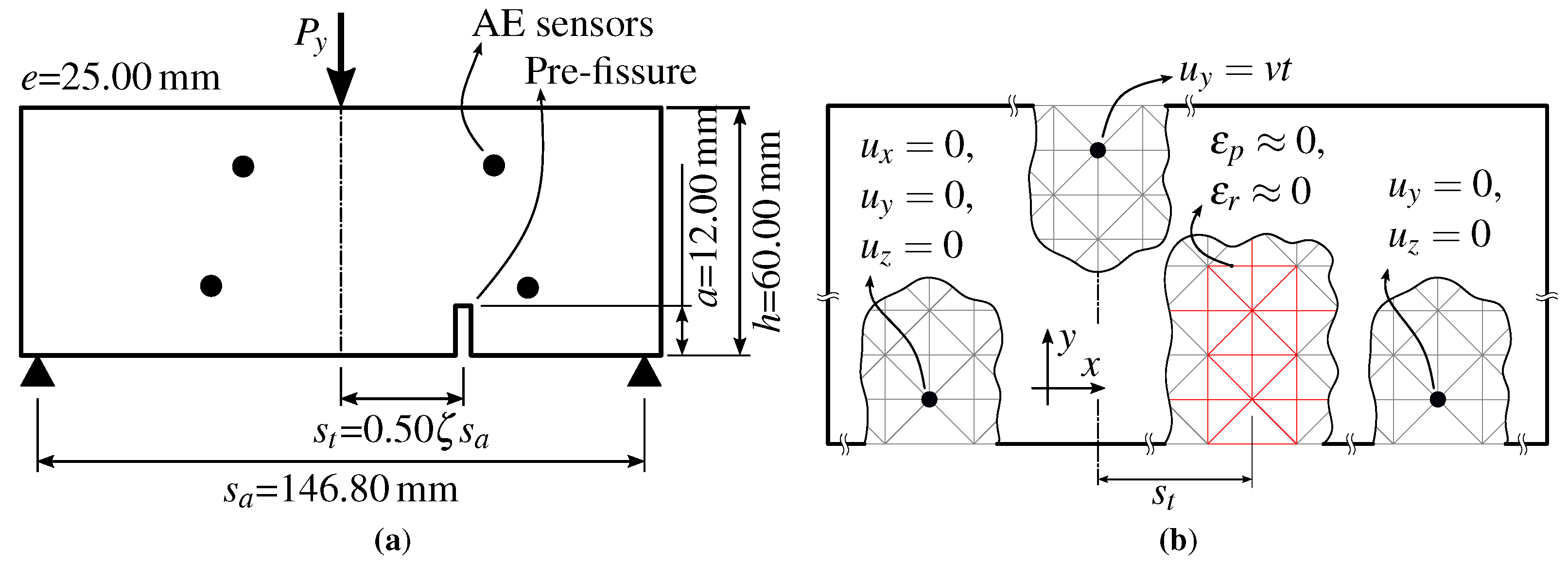
  • Subjecting a pre-fissured sandstone beam to a three-point-bending test, carried out experimentally by [41], as well as through simulations performed in this study. The simulated dataset was then used to deepen the understanding of the damage process through comparisons with the corresponding experimental data.
The overall purpose was to illustrate how the synergistic use of these two strategies (LDEM and AE) could lead to a more comprehensive understanding of damage processes and could be employed an invaluable analysis approach for studying quasi-brittle structures.

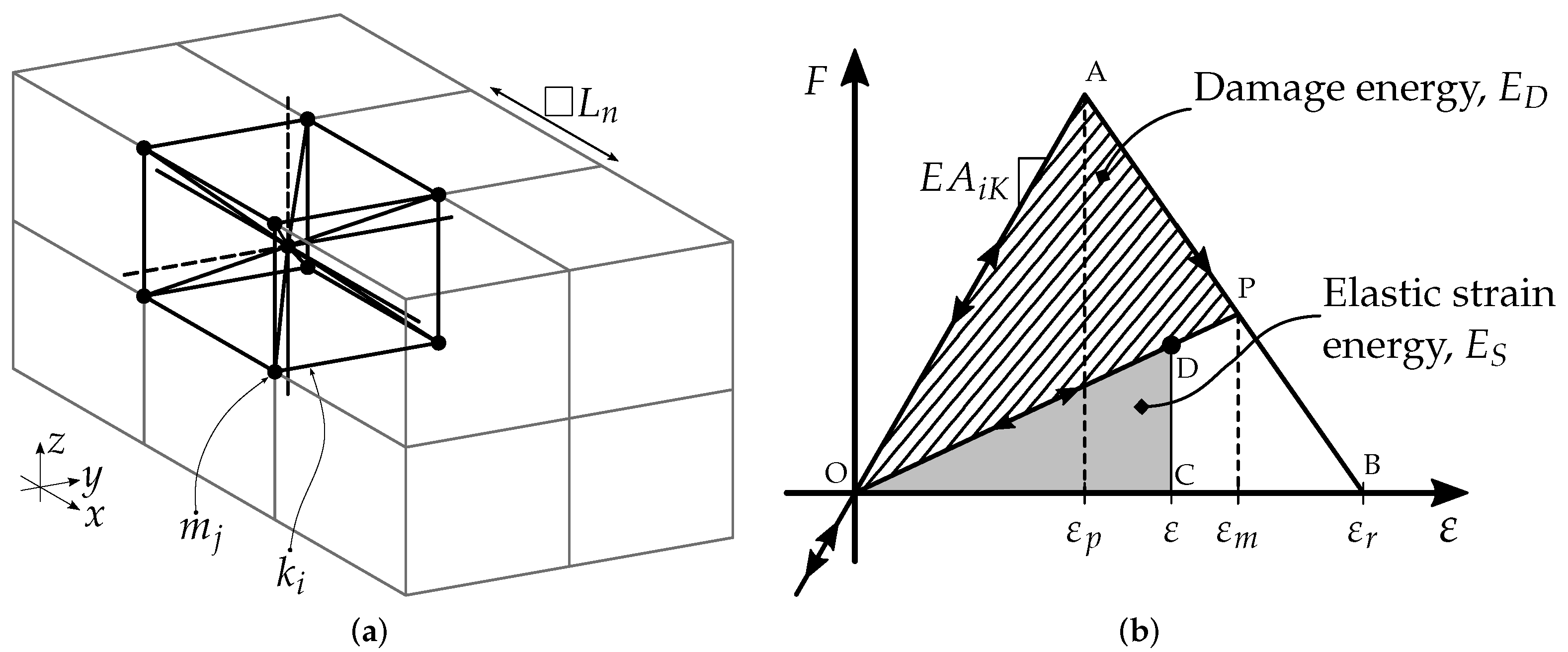
2. Overview of the LDEM Approach

The LDEM approach modeled solids as a set of mass-less uni-axial elements and nodal masses, forming cubic cells of 20 bars and 9 nodes, as depicted in Figure 1a. Each node had three degrees-of-freedom, corresponding to its displacements in each coordinate direction. The lengths of each longitudinal and diagonal element were denoted as L n and L d = 3 L n / 2 , respectively. The equations relating the properties of the LDEM elements to the elastic isotropic medium were as follows:
δ = 9 ν 4 8 ν , α = 9 + 9 δ 2 9 + 12 δ ,
A n = α L n 2 , A d = 2 3 δ α L n 2 ,
where E and ν denote the Young’s modulus and Poisson’s ratio, respectively, of the material, whereas the initial axial stiffness values of the normal and diagonal elements are E A n / L n and E A d / L d . Equations (1) and (2) were proposed by Nayfeh and Hefzy in [26], and their derivations within the context of the lattice element method used here were complemented in [42]. For ν = 0.25 , the cubic array in Figure 1a yielded the exact representation of the isotropic continuum, while the other values of ν caused small differences to appear in the shear values [26]. The motion equation was enforced at every node to obtain the following,
M u ¨ + C u ˙ + f p = 0 ,
where u is the vector of the generalized nodal displacements, M is the diagonal mass matrix, C is the damping matrix, and f and p represent the internal and external forces acting on the nodal masses, respectively. If M and C are diagonal, the system is not coupled, and the explicit central finite differences could then be used to integrate the equations of motion in the time domain. As a result, since the nodal coordinates were updated at every time-step, large displacements were innately handled. The softening law for quasi-brittle materials proposed by [43] was implemented by the triangular-element constitutive relationship (OAB) of the LDEM longitudinal and diagonal elements (Figure 1b), which accounted for the irreversible effects of the crack nucleation and propagation. To ensure that the overall formulation was diagonal, the model’s damping was assumed proportional to the mass, as follows:
C = D f M ,
where D f is a damping coefficient for filtering unwanted higher frequencies in the numerical simulations. The most effective approach for its determination remained an open issue in LDEM applications. For example, in [44,45], this coefficient was calibrated by the direct comparison with experimental measurements from global damping specimens. The numeric model was simulated under the same loading and boundary conditions from the experiments, and D f was chosen so the model’s logarithmic decrement matched the experimental values. An alternative approach was to modify the LDEM’s uni-axial constitutive law by including a visco-elastic term that depended on the strain velocity. Here, D f 2 π f m ζ m was estimated from the model’s energy spectrum, where f m and ζ m represent the natural frequency and damping ratio of the highest energy peak, respectively. This approach was also used in [46], which explores the influence of D f in more depth in the application of LDEM for modeling wave propagation in soils.
Figure 1b describes the constitutive law assumed by the LDEM model for the force exerted by a bar as a function of its strain, where ε p denotes the elastic limit strain, ε m is the maximum strain experienced by the element up to that point, and ε r is the critical failure strain. Since the area under the curve was proportional to the energy accumulated by the bar under strain, for a given point P, the area of the triangle OAP (striped sector) would be proportional to the energy dissipated by the damage, whereas the OCD (gray area) would be related to the elastic strain energy stored in the bar. If the external load was relaxed at point P, the return slope would be lower than the initial slope because the bar would then be partially damaged. When ε = ε r , the damage energy density would equal the fracture energy, and then the element would fail and lose its load-carrying capacity. Each element’s equivalent fracture area A i * was chosen to ensure that the energy dissipated by continuum fracture matched its discrete representation. For this purpose, the fracture of a cubic sample of dimensions L n × L n × L n was considered. The energy dissipated by a cubic LDEM module and its distribution in the various elements were examined by [47], with an alternative constitutive relation proposed in [48]. Under compression, as the material was assumed to remain linearly elastic with an initial slope E A , failure would be induced by indirect tension. In a quasi-brittle material, tensile collapse stress is commonly reached at around 1/10 of its compressive strength. Therefore, the model could capture compression effects indirectly without considering compression-induced damage because tensile failures are the most common. Shear effects had to be considered in order to capture the post-failure behavior, as discussed extensively in [27]. Further discussion on the representation of compression effects on concrete using LDEM were also found in [49].
As described comprehensively by [50], there were two approaches for representing the material’s random micro-structural features, either separately or simultaneously:
  • Introducing small disturbances throughout the mesh with the node coordinates ( x , y , z ) defined by:
    ( x n + r x L n , y n + r y L n , z n + r z L n )
    where x n , y n , and z n are the node coordinates for a perfect cubic array, whereas r x , r y , and r z are normally distributed random numbers with zero mean and variation coefficient C V p .
  • Defining the material’s specific fracture energy G f as a random 3D-field, according to a Type-III (Weibull) distribution, where the mean and the variation coefficient would appear as input parameters. This option also considered a spatial correlation ( l c ) for G f when l c > L n .
In addition to the aforementioned approaches, the strains ε p and ε r (see Figure 1b) were related the material’s characteristic length d e q , as follows:
ε p = G f E d e q ,
ε r = ε p d e q A i * A i 2 L i .
In Equation (7), A * was each element’s equivalent fracture area, defined to ensure that the energy dissipated by the fracture of the continuum was equal to that of its discrete counterpart. The sub-index indicated the type of element referenced (diagonal or normal). Finally, the characteristic length was especially relevant because it represented the minimum fissure dimension for an unstable fracture to start propagating. According to [51], this length also related to other significant parameters, such as fragility s:
s = G f E d σ p ,
where d represents the characteristic length of the structure and σ p is the failure stress. Combining Equations (6) and (8), we obtained the following:
s = d e q d ,
where d e q depends on the characteristic length ( d m ) of the material, proposed by [52], and given by:
d m = ε p d e q ,
these relations are discussed in more detail by [49,53].
In another version of the discrete element approach called Peridynamic, as proposed by [11], the structure was treated as an arrangement of punctual discrete masses that represented the density of the continuum, with the functions of the interactions emulating the links between these points. The level of neighboring (interactions) among nodes was given by the material parameter called horizon, whose physical meaning was analogous to d e q . The peridynamic approach was used in [24,25], with a constitutive law similar to the one we adopted in this study.
All LDEM models used here were implemented with proprietary codes in Fortran, as discussed in further detail in [54].

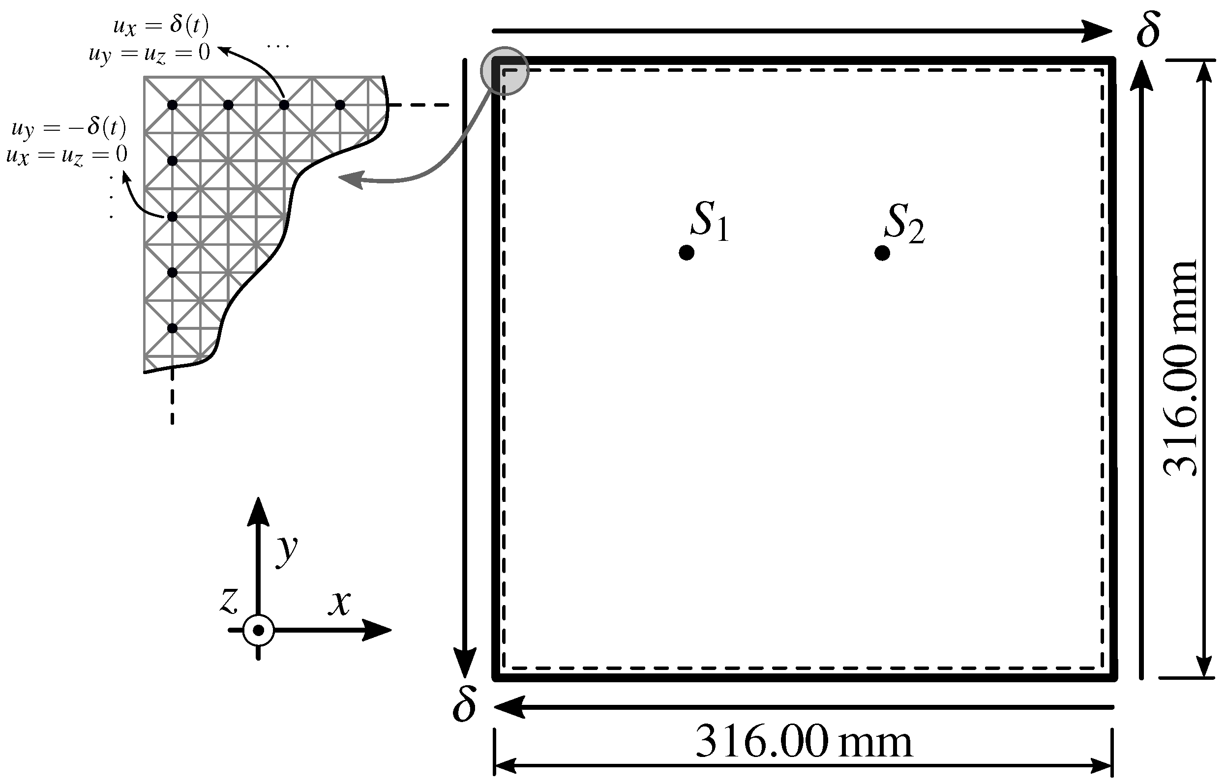
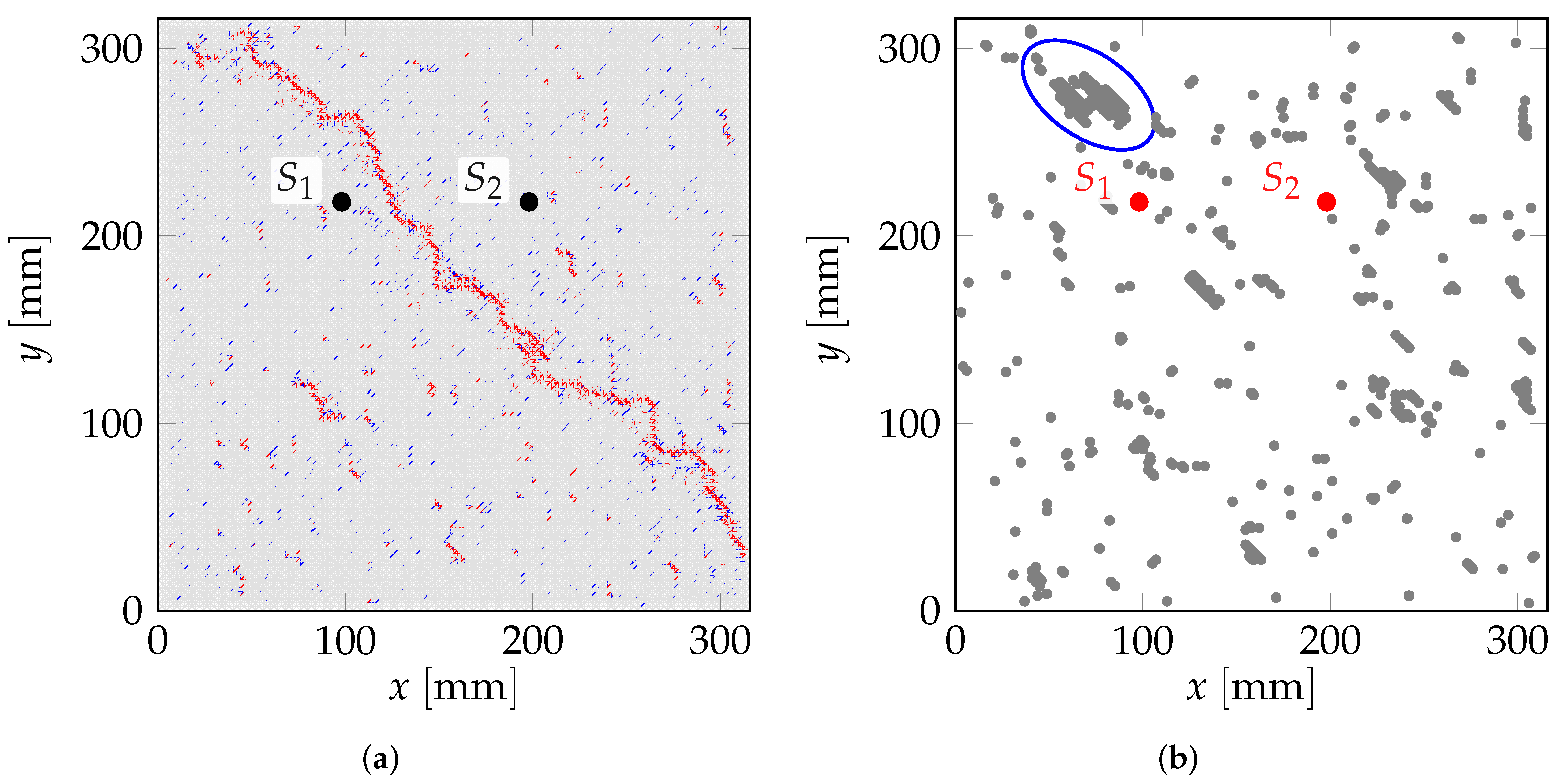
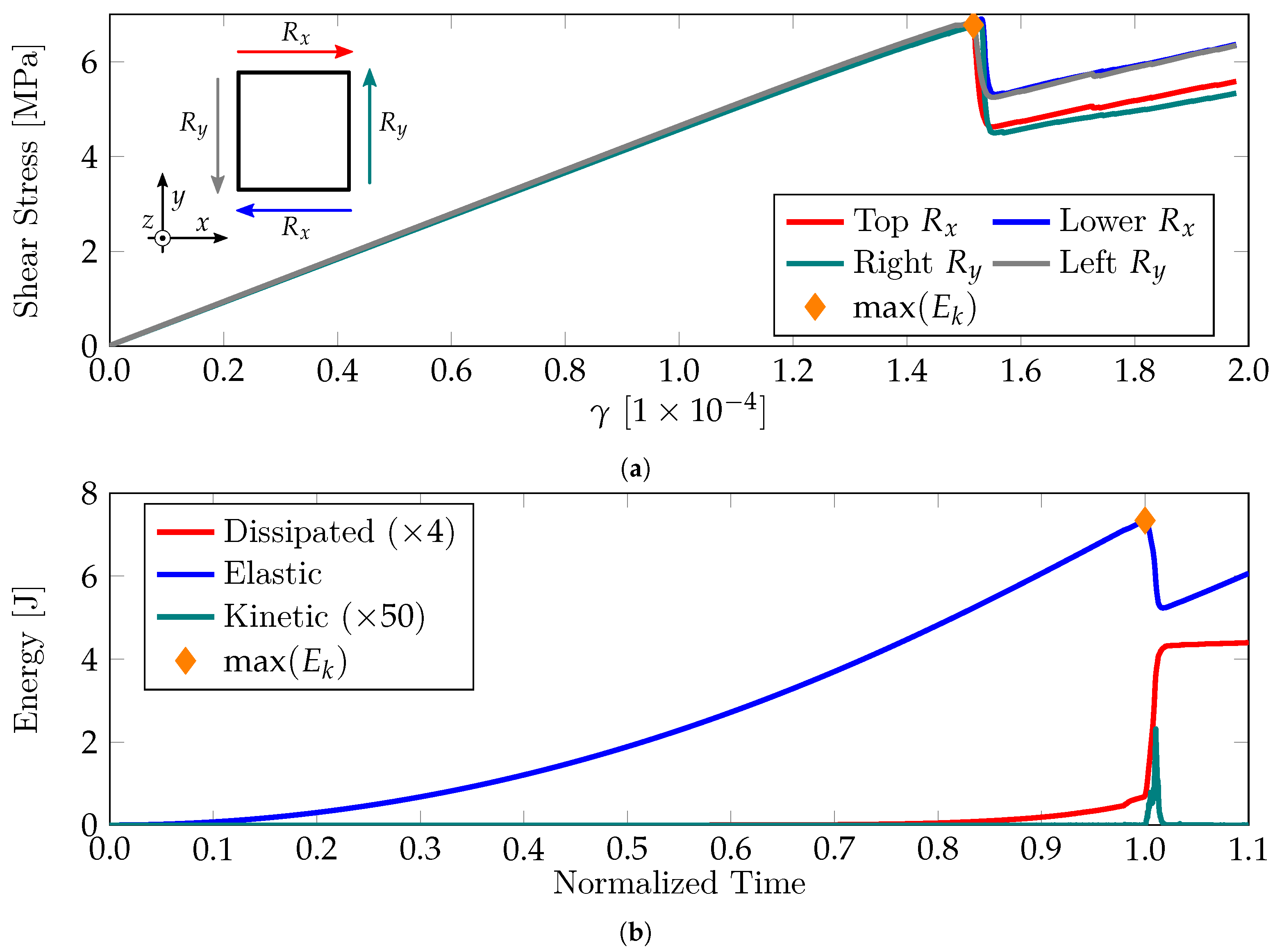
3. First Application: AE Events in a Simulated Fracture Process

Before discussing the experimental data in Section 4, we evaluated the proposed LDEM approach through an entirely simulated test. It concerned the fracture process of a square plate subjected to prescribed displacements, thus inducing a nominally homogeneous pure-shear load with linearly increasing amplitude. The corresponding damage process was evaluated through virtual AE events generated by the acceleration waves induced within the structure as cracks occurred. The same structure had been previously studied by [55], using uni-axial and shear stresses to evaluate the influence of the LDEM mesh orientation on the damage process simulation. In this study, the main focus was to analyze how the internal ruptures (events) generated the signals captured by the virtual sensors.

3.1. Model Description

This simulation described a concrete-made, 316 m m long by 36 m m thick square plate, as shown in Figure 2 with its prescribed boundary conditions. The figure also includes the positions of virtual AE sensors, simulating accelerometers aligned with the direction normal of the plate’s median plane. The corresponding LDEM model comprised 79 × 79 × 9 cubic cells, with L n = 4 m m . All other relevant parameters are shown in Table 1.
In Table 1, d e q = 0.022   m was obtained by assuming σ t = 10 M Pa , G f = 70 N / m −1, E = 32 G Pa , and d = 0.316   m , in Equation (8), yielding s = 0.27. Therefore, replacing s in Equation (9) resulted in the adopted d e q . As that parameter was much smaller than the plate’s characteristic dimension d = 0.316   m , brittle behavior was expected. We also observed that the chosen σ t was slightly higher than the real value for concrete, as it was selected to emphasize the model’s fragile behavior and to facilitate the identification of AE events.
For the random field, the coefficient of variation was determined according to [48], which showed that C V ( G f ( s o l i d ) ) = C V ( G f ) / 2.5 for the LDEM’s cubic arrangement. Therefore, C V ( G f ( s o l i d ) ) = 100 / 2.5 = 40 % in the present case. The correlation lengths l c x , l c y , and l c z were considered equal to the cubic module’s side. Random mesh variability was introduced as the normally distributed perturbation with C V p = 2.5 % . This was based on [56], which stated that this value had to be smaller than 2.75% and suggested 2.5% as a typical value for concrete. The introduction of randomness in the LDEM was discussed in more general terms by [50].

3.2. Results

The first results referred to the overall damage. As shown in Figure 3a, the final simulated configuration showed a main diagonal fissure throughout the plate, which was typical for this test. That information was complemented by the distribution of bars that surpassed their limit strain ε r , from the start of the process to immediately before the main fracture occurred (Figure 3b). As shown in Figure 3b, a distinctly dense cluster of broken bars (a crack) appeared where the main fissure began. This region’s dimensions were nearly 0.022   m , which was consistent with the value of d e q in Table 1 and its definition in Section 2, i.e., the critical crack size that would generate unstable propagation throughout the specimen.
Figure 4a illustrates the same test regarding the shear stresses along each plate edge as a function of the distortion angle. Due to the non-homogeneous nature of the material, the homogeneous stress state was perturbed once the first micro-fracture had appeared. Afterwards, it remained approximately homogeneous until the peak load was reached. Then, unstable fracture propagation took place, leading to large changes in the stress distribution. We noted that the test concentrated on the damage process leading to collapse, so the post-peak behavior was not considered. The corresponding energy balance is shown in Figure 4b. The sudden increases in kinetic and dissipated energies after the normalized time of 0.80 were clear indicators of unstable growth in the main fissure that had nucleated during the damage process.
We then analyzed the same results in terms of the AE signals captured by the virtual sensors S 1 and S 2 . As shown in Figure 5, the analysis was performed according to the b-value parameter, which has been widely used in seismology in connection with the Gutenberg–Richter (G-R) law [57]. As damage progressed, the acoustic waves appeared within the structure as the fissures were formed. These wave amplitudes were a measure of the fissure sizes and, therefore, of the damage extension. Mathematically, each wave connected with an event, and the G-R law determined that the cumulative number N of events with amplitudes larger than or equal to a given cutoff amplitude A, according to the following:
N ( A ) = c A b .
Otherwise, in the bi-log domain:
N ( A ) = log ( c ) b log ( A ) ,
where c and b reflect both the intrinsic material properties and the boundary conditions applied to the structure, respectively. This relation has been widely investigated in several works, such as [19,21,22]. In particular, ref. [29] interpreted the b-value as one-half of the fractal dimension of an AE event. According to this interpretation, during the damage process, the b-value was expected to change from an ideal initial value around b = 1.5 (D = 3) to a final result close to b = 1.0 (D = 2), because the individual (punctual) micro-fissures tended to combine with the main crack.
As shown in Figure 5, the calculation of the b-value was superposed to the AE amplitude distribution during the simulated process. We noticed the sharp decrease in the b-value as the AE activity increased, which agreed with other works, such as [39] and the seismic records of the Aquila region in Italy, as described in [58].
Figure 5. Correlation of b-value variations with the AE amplitude distribution during the simulated fracture process.
Applsci 13 05119 g005
Figure 6 depicts the AE signals from the virtual sensors S 1 and S 2 captured during the test. Two events were highlighted: one at the beginning of the damage process and the very last event before the rupture. This information was complemented by the number of broken bars during the time interval of each event: (0.504, 0.512) for event 1 and (0.979, 0.987) for event 2. We observed that event 1 was associated with the rupture of only 1 bar, whereas several broken bars appeared for event 2. The link between event 2 and the space–time distribution of the broken bars is shown in Figure 7 and Figure 8.
In Figure 7, the responses of the two highlighted events in Figure 6 are shown in more detail. The delay between an AE event and its corresponding energy increment was due to the traveling of the elastic wave from the perturbation source to the virtual sensor. We noted the differences in the magnitudes due to the number of broken bars: only 1 for event 1 and about 1000 for event 2. We also observed that the signal from S 1 suggested that event 2 could be regarded as 2 events separated by a brief period of silence.
Figure 8 depicts the spatial distribution of energy increments for event 2, between the 0.980 and 0.986 instants of normalized time. We noted the high amount of elastic energy at the event’s end, indicating its tendency towards continued propagation during the process. Moreover, two primary sources were identified in the event’s buildup, reinforcing the concept that it could be treated as two separate events: one produced by the blue and light-blue broken bars and another from the yellow to the red broken bars.
In Figure 9, the simulated damage process is illustrated through increments of kinetic and dissipated energies, i.e., Δ E i = E i t + d t E i t , where d t is the integration time-step, and E i t + d t and E i t are the energy values in 2 successive steps, with a sub-index indicating whether they were dissipated or kinetic energy. We noted that the peaks of the incremental kinetic energy coincided with the AE events indicated by the virtual sensors, which was expected because the AE events were directly related to the kinetic energy, i.e., the “energy that makes noise”, according to [59]. Furthermore, as shown in Figure 9, the energy had dissipated in two ways: smooth or spasmodic. The latter was associated with avalanches of the dissipated energy that also contributed to the local kinetic energy increments. A thorough discussion of the correlation between the energy increments and the acoustic emission signals was found in [60].

4. Second Application: Three-Point Bending Test and Comparison to Experimental Data

In this section, the damage to the two Berea Sandstone beams was simulated with an LDEM model. The simulated results were evaluated through a direct comparison with the experimental AE data by [41].

4.1. Model Description

The beam geometry and the sensor positions are shown in Figure 10a, where ζ = 0.0 and 0.4 defines the fissure’s position in each case. A three-point-bending test was performed by controlling the displacement velocity in the fissure’s mouth (CMOD). The boundary conditions are shown in Figure 10b, which also illustrates how the main fissure was modeled in the numerical model: The bars’ constitutive laws were modified, reducing their corresponding strength values.
The respective LDEM model was built with 73 × 27 × 12 cubic modules, with sides of 2.25   m m , that were excited through a constant-velocity-prescribed displacement. The model parameters were based on those in [41] and presented in Table 2. Two pre-fissure configurations were considered with s t = 0.5 ζ s a , where ζ = 0 and ζ = 0.40.
Important considerations regarding the model calibration were as follows:
  • The Young’s modulus for Berea Sandstone, as presented in [41], was in the range from 12 G Pa to 15 G Pa . In this study, it was considered 15 G Pa to better adjust the curve force vs. global vertical displacement, as shown in Figure 11 (red line).
  • G f was considered a random field with a Weibull distribution, with a mean value computed by considering P c r i t = 736.8   N , as shown in Figure 11, and using the classical fracture-intensity factor expression for the three-point-bending test, as provided in Equations (13) and (14) [61], yielding K I c = 345,860 Nm 3 / 2 , and G f = K I c 2 / E = 7.9   N m 1 .
    K I = P y e h f a h ,
    where
    f a h = 3 S a h a h 2 1 + 2 a h 1 a h 3 / 2 1.99 a h 1 a h 2.15 3.93 a h + 2.7 a 2 h 2 .
  • The material porosity used by [41] was in the [0.1 mm–0.8 mm] interval, which was lower than the discretization level adopted in this study. For this reason, we assumed l o = l c , meaning that the random generation of each bar would be statistically independent. However, in the same reference, the variations in the tensile stress test were about 6% ( σ u = [3.4 MPa–3.6 MPa]), whereas it was around 10% in [62] for sandstone specimens with the same dimensions. Previous studies using LDEM on tensile specimens with similar sizes showed that to obtain a C V ( σ u ) close to 10%, the bars’ C V ( G f ) had to be about 65%. The links between the toughness random field properties and the global parameter variations were discussed in more detail in [50,63].
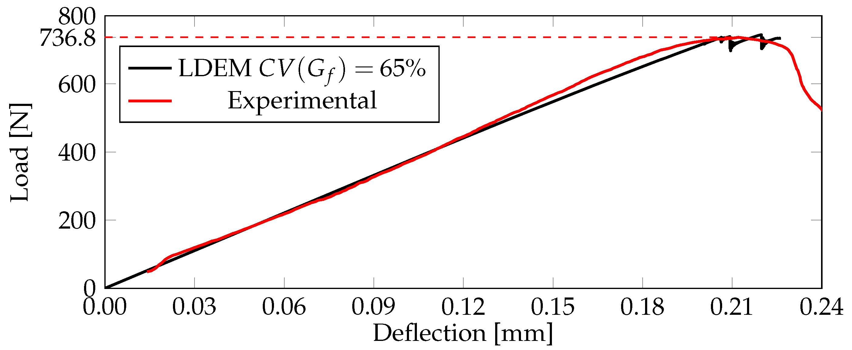
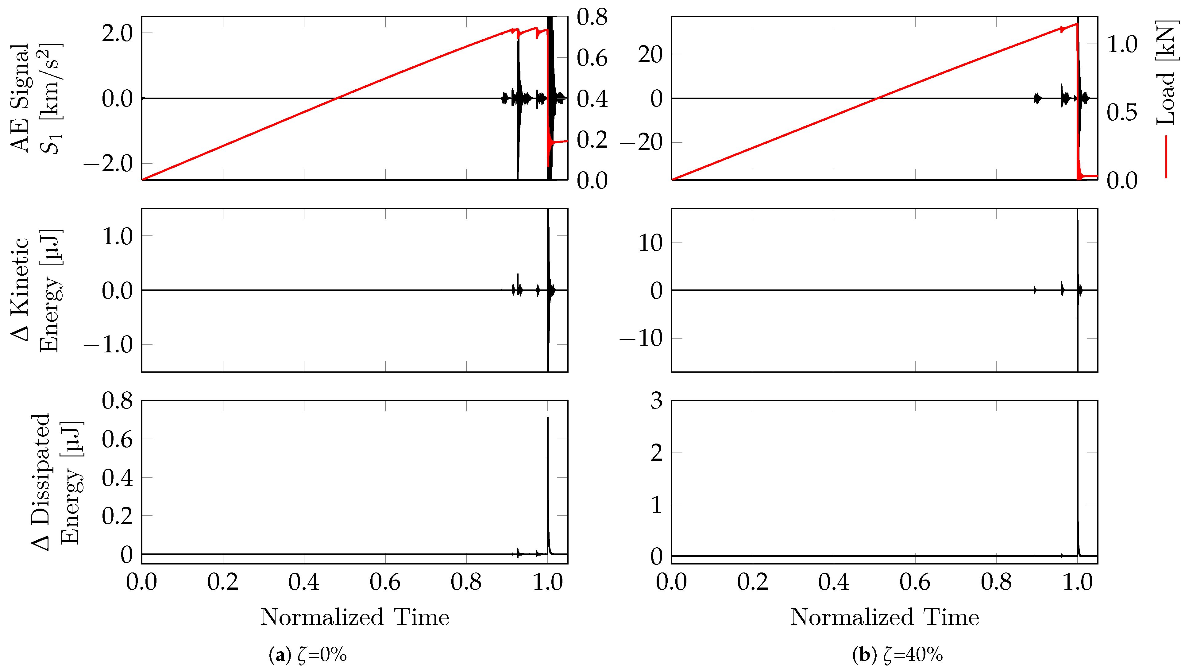
  • The material’s characteristic length d e q was based on the Carpinteri number, assuming σ p = 3 MPa. This parameter was slightly lower than the range used in [41] [3.4 MPa–3.6 MPa], and slightly higher than the values presented by [62]. The corresponding value for s was computed using Equation (8):
    s = G c E d σ p = 7.3 N   m 1 15 G Pa 0.06 m 3 M Pa = 0.45 ,
    Then, based on s and using Equation (8), we obtained d e q = s 2 d = 0.45 2 × 0.06   m = 0.012   m . For a detailed discussion between d e q and s, see [53].

4.2. Results

The results from the simulated model are shown in Figure 11, Figure 12, Figure 13, Figure 14, Figure 15 and Figure 16. In Figure 11, simulation results are directly compared to the corresponding experimental results obtained by [41], for ζ = 0%. The best approximation from the numerical model occurred when C V ( G f ) = 65%, as observed in Section 4.1.
Figure 12 depicts the progression of the AE events in normalized time, accompanied by the load applied to both configurations. The simulated increases in the kinetic and dissipated energies are also presented. As in Section 3, there was a clear correspondence between the identified AE events and the energy spikes that signaled damage.
Figure 13 illustrates the global energy balances of the two configurations. The structure was more fragile when the fissure was not centered ( ζ = 40%), which was corroborated by the sharper spike in the damage energy in the off-centered case.
Figure 14 illustrates the simulated configurations immediately before and after the main fissure’s unstable propagation. Damaged elements (i.e., those with ε ε p ) are in blue, whereas the fractured elements (when ε ε r ) are in red. For the centered case (Figure 14a), a spasmodic local failure appeared at the normalized instant t = 0.85, which was identified as many damaged bars around the pre-fissure’s head and confirmed by the energy balance in Figure 13a. It was also apparent that the non-centered case generated many more broken and damaged bars than the centered example. That was also confirmed in Figure 13: the energy dissipated by damage was nearly 50% greater than the non-centered pre-fissure. Finally, it was also clear that the energy had dissipated due to the final collapse because the ζ = 40% configuration was substantially higher than that of ζ = 0%, as evidenced by the number of damaged/broken bars (Figure 14a,b) and the corresponding variations in the dissipated (i.e., damage) energies in the energy balance at the failure instant, as shown in Figure 13.
The simulated acoustical energy release was calculated in the same way in these tests, as described in Section 3.2, and then compared to the experimental results in [41]. The corresponding energy values for the latter were estimated from the AE data according to E A max 2 , where A max is the maximum amplitude of each AE signal, and their spatial localization was performed through the standard procedure according to [31]. The comparison between the experimental and simulation results is shown in Figure 15 and Figure 16, considering the events between 0.9 and 1 in normalized time. When the fissure was displaced from the center by 40%, it became inclined with respect to the applied load. Therefore, a new coordinate system was established, with its origin at the tip of the fissure and aligned with the expected fracture path. Mathematically, these coordinate transformations were expressed as follows:
x 0 = x cos ( ψ ) ( y 11 ) sin ( ψ ) y 0 = x sin ( ψ ) ( y 11 ) cos ( ψ )
where all displacements are given in mm. The angle ψ corresponded to the inclination of the fracture path, as shown in Figure 16d, as 27.8   for ζ = 40%. At first, the simulation results suggested a significant deviation from the experiment due to the large number of AE events that occurred left of the origin, as shown in Figure 16a. However, such events were relatively sparse, as compared to those immediately around the fissure, indicating that most of the AE emissions tended to be concentrated in the same region, as in the experiment. We confirmed this conclusion by generating the corresponding histograms for the new coordinate system and observing that most AE events had aligned with the “tilted” y-axis, i.e., along the fracture’s path.
Overall, the localization of events and the energy distribution yielded by the simulated models agreed with the experimental results in [41], indicating that the proposed LDEM approach was a valuable tool for analyzing damage in quasi-brittle structures. However, a few relevant discrepancies were noted:
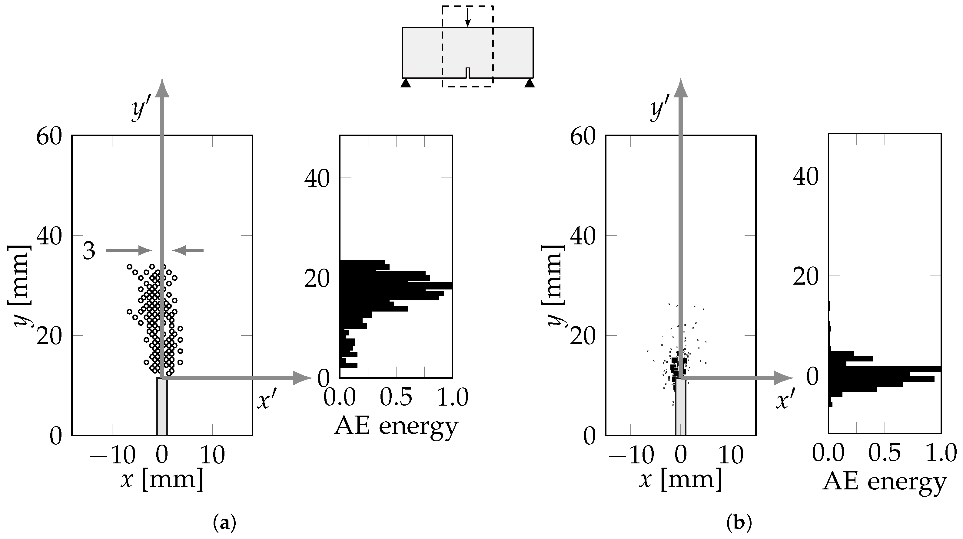
  • A significant part of the experimental AE events occurred below the pre-fissure’s head, whereas almost none appeared in the LDEM simulation. That difference was probably due to unintended damage in the pre-fissure region during the specimen preparation.
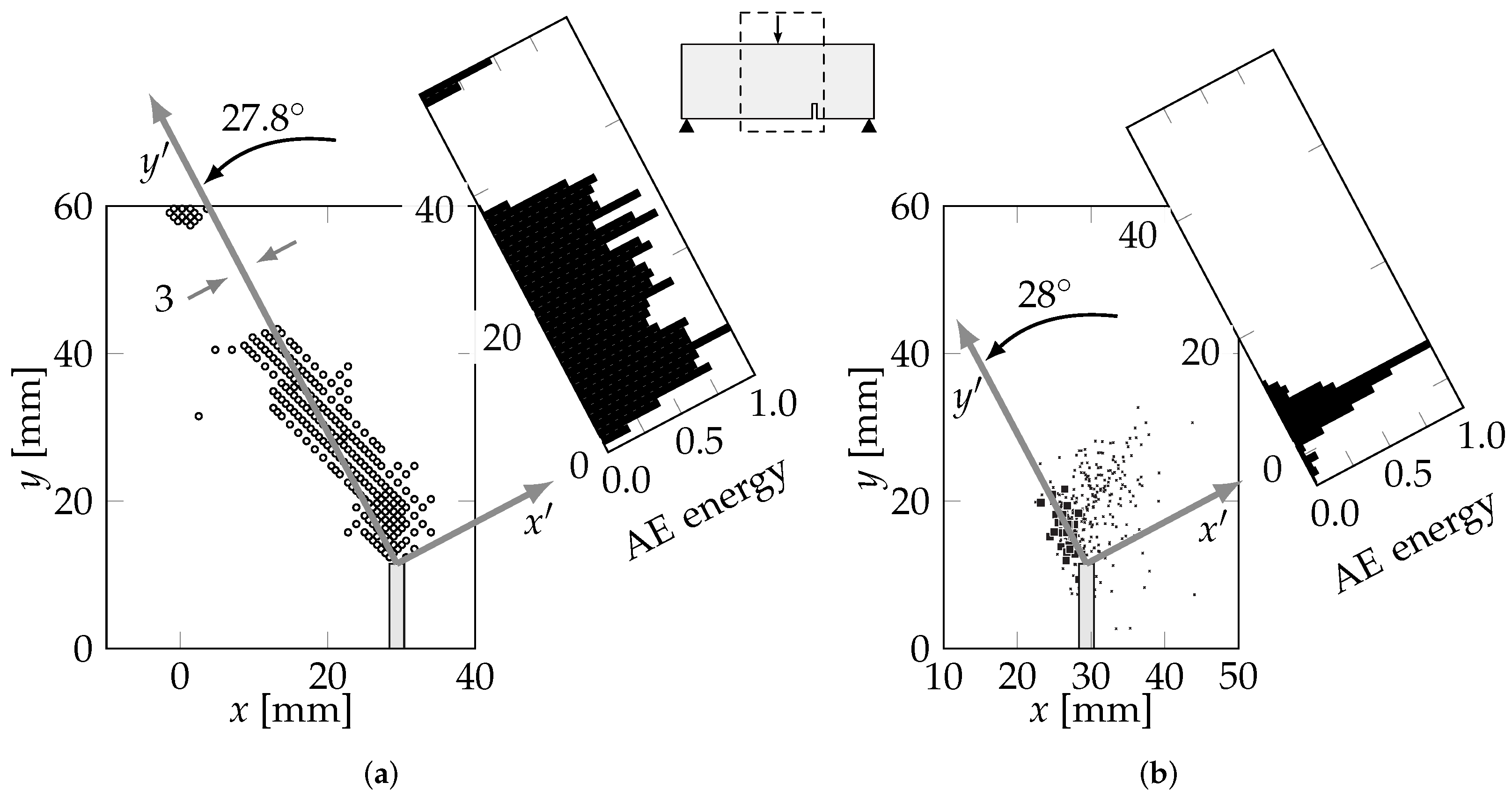
  • The simulations indicated noticeable AE activities in regions other than along the main crack, such as in the vicinity of the load application (both tests) and in the horizontal direction crossing the top of the main fissure’s head (non-centered case). No such activity occurred in the corresponding regions during the experiments. These discrepancies were probably derived from the determination methods for identifying AE activity: The events in the numerical data were calculated from the kinetic energy produced inside the model, free from the attenuation that affected the signals captured by the sensors.

5. Conclusions

In the present work, the damage process of quasi-brittle materials was studied using the acoustic emission (AE) technique and a version of the lattice discrete element method (LDEM).The effectiveness of combining the two approaches was explored through two applications, each illustrating different aspects of these analysis tools. The most important observations from each application were the following:
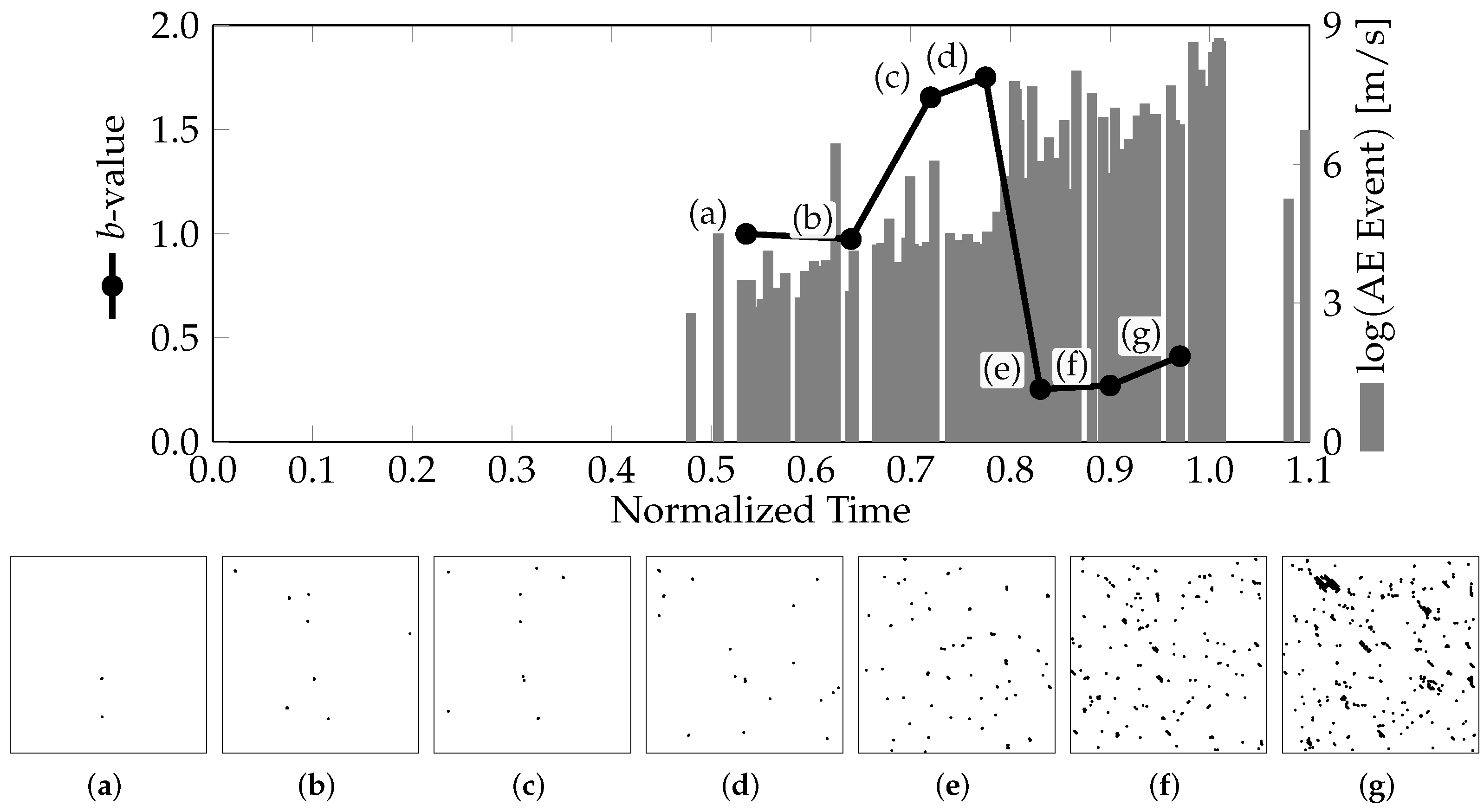
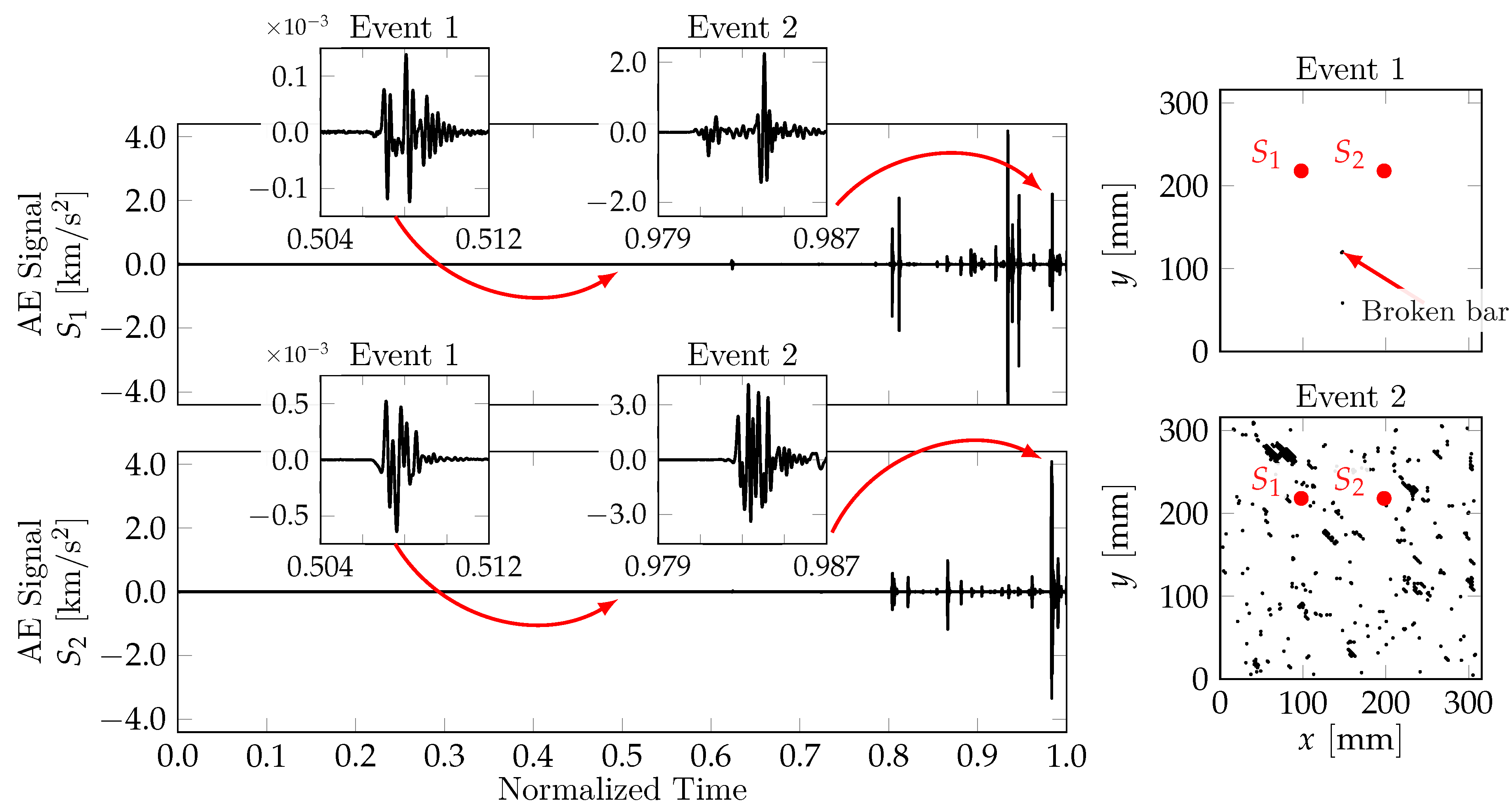
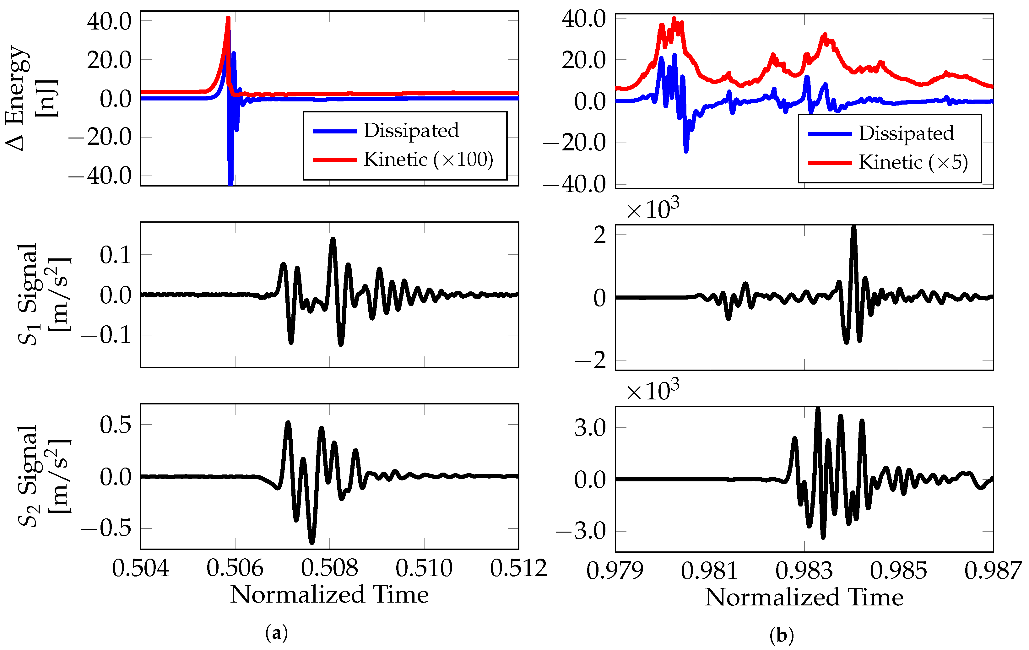
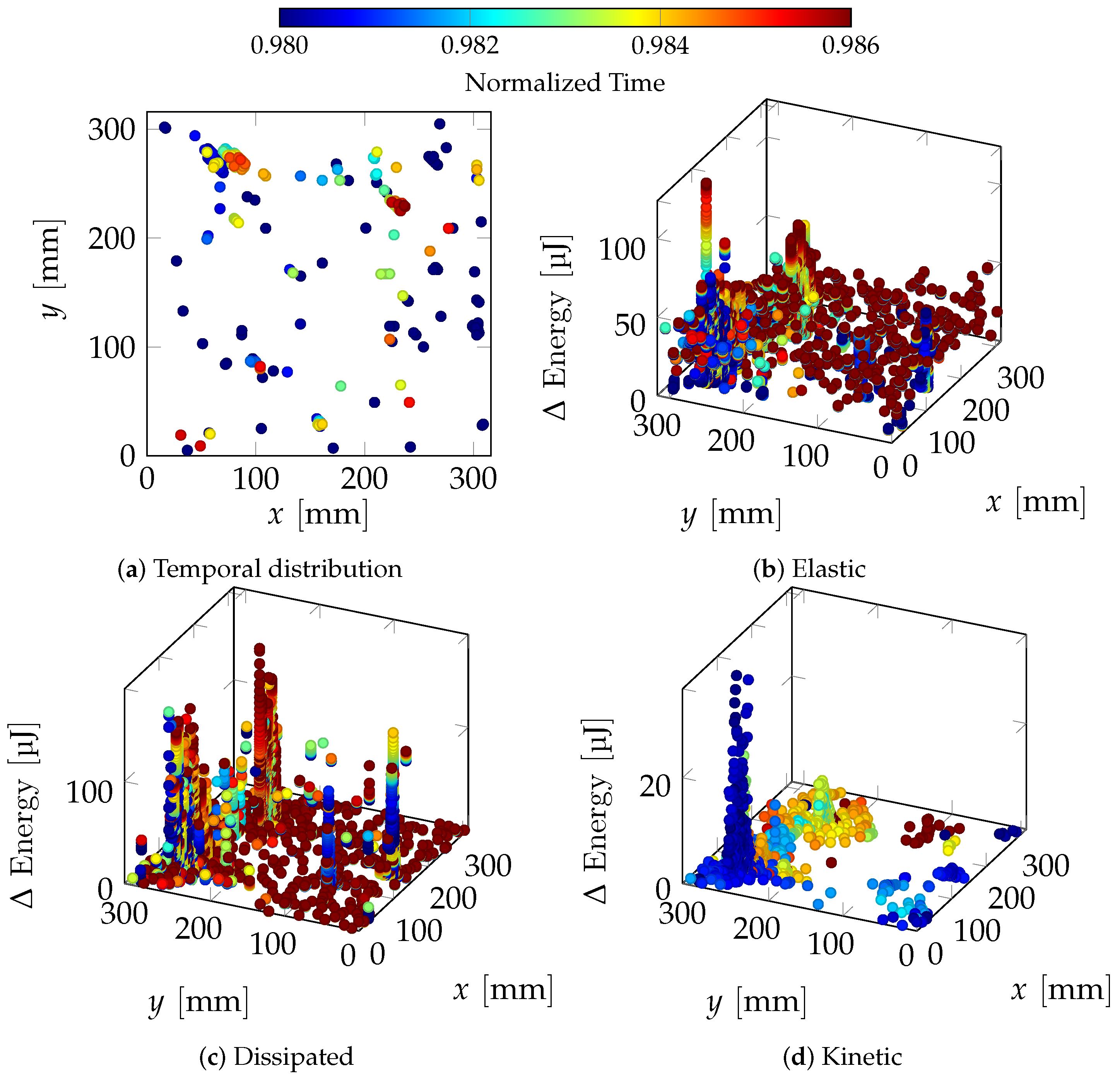
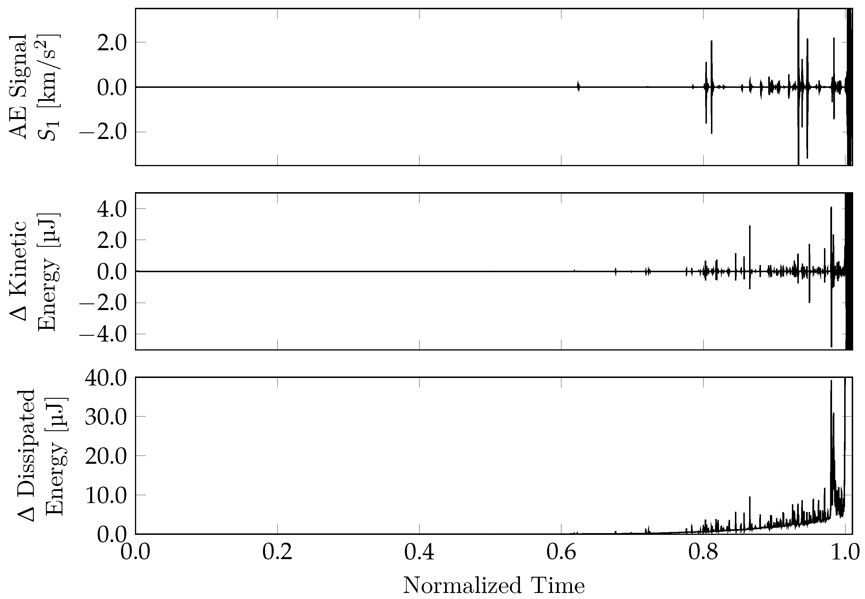
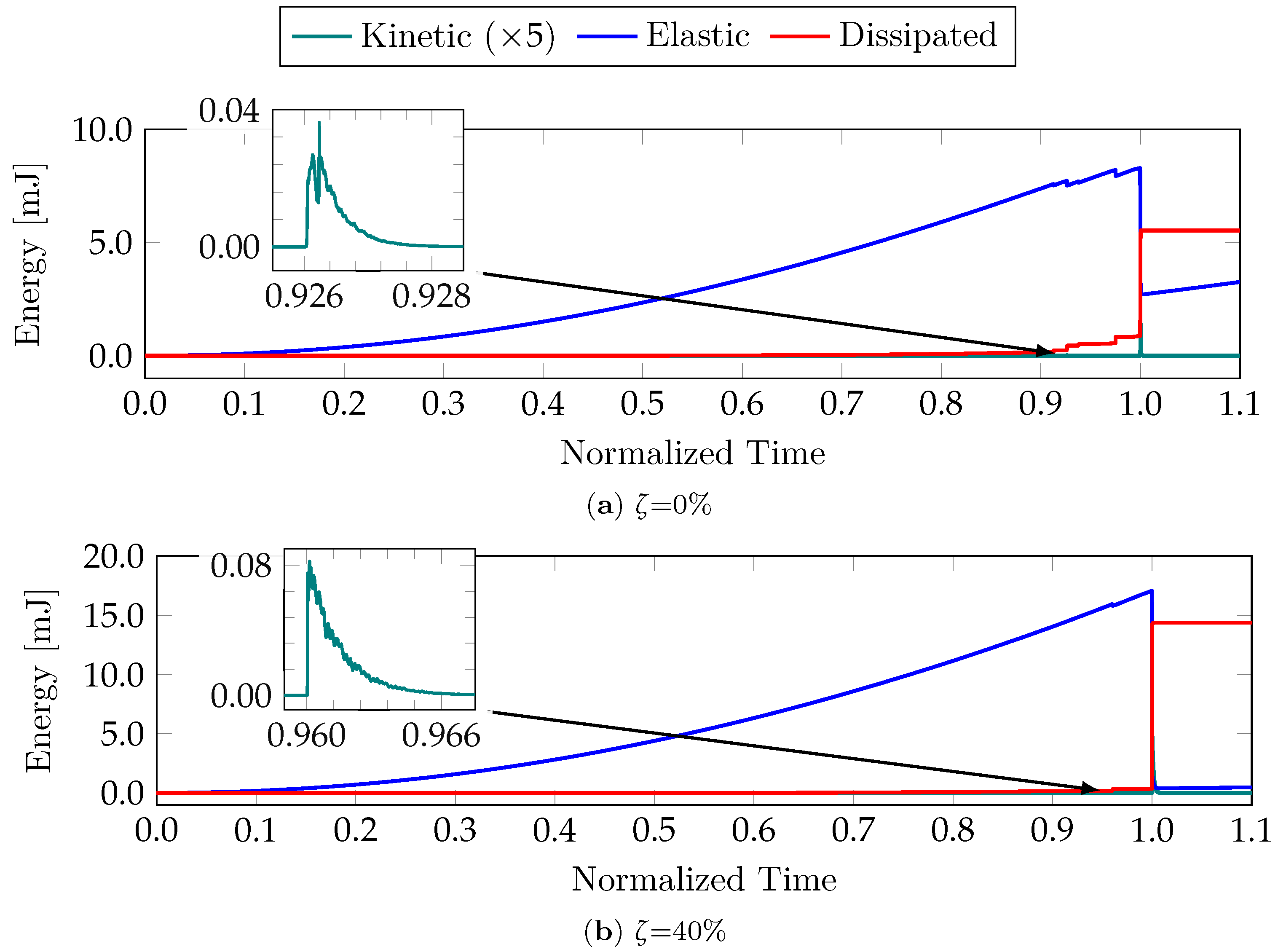
  • The first study used simulations to illustrate the LDEM’s ability to emulate the typical results of AE tests, such as the spatial and temporal distributions of signals captured by AE sensors. It also yielded the calculations of the global parameters usually employed in AE methods for predicting local and global damage-induced instabilities.
    Those parameters were complemented by capturing the temporal and spatial distributions of the simulated elastic, dissipated, and kinetic energies involved. These were then used in an inverse analysis, linking the signals from the virtual AE sensors with the element-breaking events that caused their emission. These signal patterns were consistent with the system’s kinetic energy progression, i.e., every large-amplitude AE signal could be traced back to a correspondingly significant variation in the energy.
    By avoiding the numerous hard-to-track variables that characterize any experimental work, this approach showed a clear cause–effect link between the damage processes and the conclusions reached in our AE-based analysis, thus confirming AE coefficients as reliable failure predictors. The extension of this concept to real-world systems is subject to the effects of many extraneous factors, reducing the effectiveness accordingly. Nevertheless, AE analysis remains a valuable method for identifying global tendencies in structures undergoing damage, as indicated by Wilson in their re-normalization group procedure [64], and in other works addressing quasi-brittle materials [1,29,30,60].
  • The second application used numerical simulations combined with the AE analysis of the experimental data from an actual pre-fissured sandstone beam undergoing damage. Here, the simulations were used not to mimic the experiment and corroborate the calculations of AE coefficients but to investigate the time–space distributions of the events, so the AE results could be linked to their probable causes in the structure’s interior as the damage progressed. The main points observed in this study are the following:
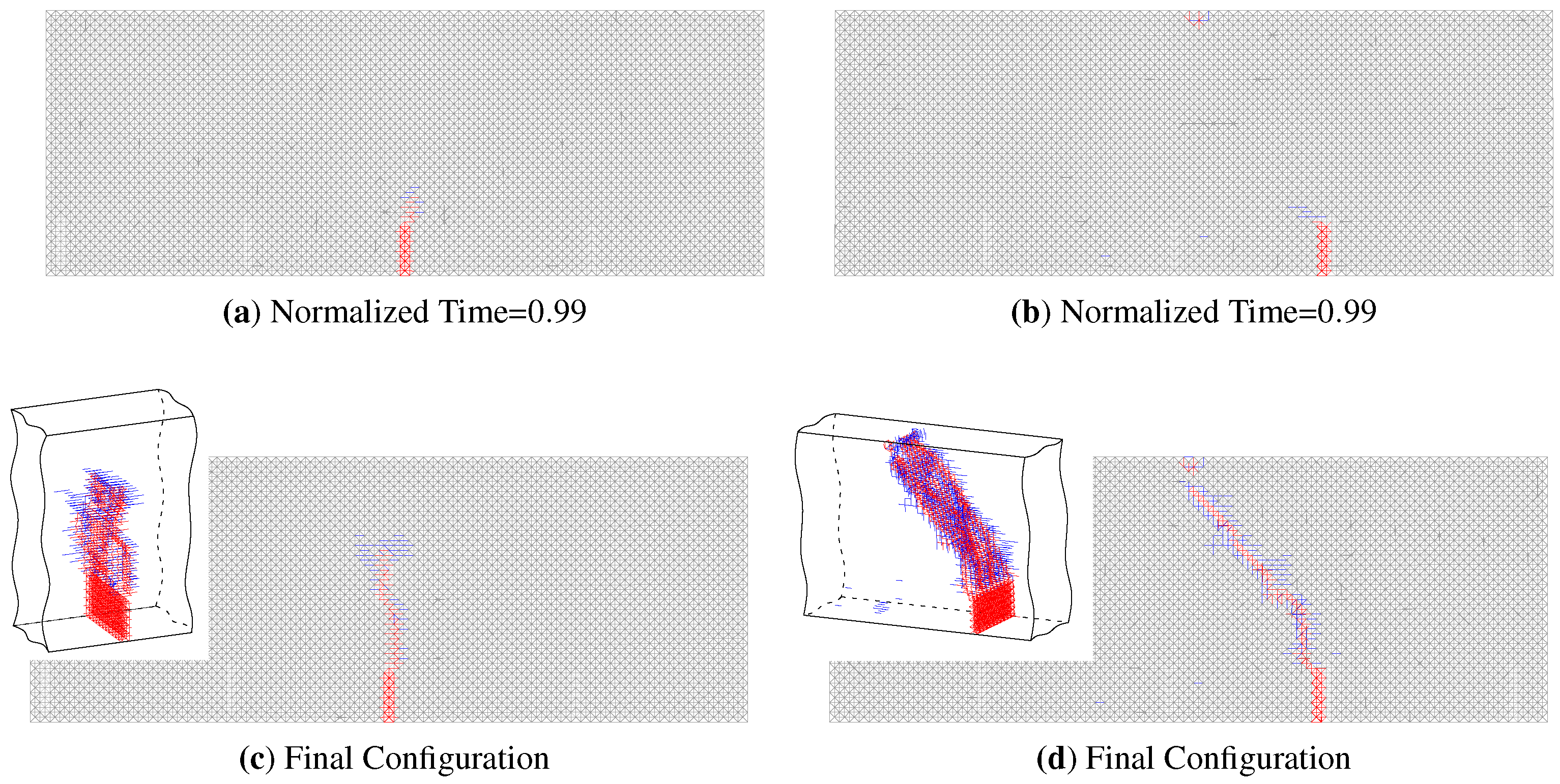
    The simulation results of the LDEM model were qualitatively similar to the damage patterns observed experimentally, especially regarding the orientation of the major cracks.
    The wave attenuation as it traveled throughout the structure was a primary limitation in identifying damage patterns through AE coefficients because it masked the corresponding signals from the data-acquisition apparatus.
In summary, the results of both tests showed that the combination of AE coefficients and LDEM models could be a valuable quantitative procedure for linking the material properties of the studied systems with their characteristic damage patterns. In particular, it highlighted the spasmodic nature of the damage processes in quasi-brittle materials, pointing to the successive formation of small, local instabilities, followed by the localization effects as the primary cause for such patterns.

Author Contributions

Conceptualization, B.N.R.T., G.B., I.I. and G.L.; methodology, B.N.R.T., G.B., I.I. and G.L.; software, B.N.R.T. and G.B.; validation, B.N.R.T. and G.B.; formal analysis, B.N.R.T., G.B. and I.I.; investigation, B.N.R.T., G.B. and M.S.; resources, I.I., and G.L.; data curation, I.I. and G.L.; writing—original draft preparation, B.N.R.T., G.B., M.S. and I.I.; writing—review and editing, B.N.R.T., G.B., M.S., I.I. and G.L.; visualization, B.N.R.T.; supervision, G.L. and I.I.; project administration, I.I.; funding acquisition, I.I. and G.L. All authors have read and agreed to the published version of the manuscript.

Funding

This research was funded by CNPq and CAPES (Brazil), and the sponsorship guaranteed the basic research funds provided by Politecnico di Torino.

Institutional Review Board Statement

Not applicable.

Informed Consent Statement

Not applicable.

Data Availability Statement

Not applicable.

Acknowledgments

The authors acknowledge the financial support received from the Brazilian National Council for Scientific and Technological Development (CNPq, Brazil) and from the Coordination for the Improvement of Higher Education Personnel (CAPES-Brazil). The sponsorship guaranteed with basic research funds provided by Politecnico di Torino, Italy, for its financial aid in this work is also acknowledged.

Conflicts of Interest

The authors declare no existing or potential conflict of interest regarding the research, authorship, and/or publication of this article.

Abbreviations

The following abbreviations were used in this manuscript:
AEAcoustic Emission
CMODCrack Mouth-Opening Displacement
LDEMLattice Discrete Element Method

References

  1. Rundle, J.B.; Turcotte, D.L.; Shcherbakov, R.; Klein, W.; Sammis, C. Statistical physics approach to understanding the multiscale dynamics of earthquake fault systems: Statistical Physics of Earthquakes. Rev. Geophys. 2003, 41. [Google Scholar] [CrossRef]
  2. Needleman, A. A Continuum Model for Void Nucleation by Inclusion Debonding. J. Appl. Mech. 1987, 54, 525–531. [Google Scholar] [CrossRef]
  3. Belytschko, T.; Chen, H.; Xu, J.; Zi, G. Dynamic crack propagation based on loss of hyperbolicity and a new discontinuous enrichment. Int. J. Numer. Methods Eng. 2003, 58, 1873–1905. [Google Scholar] [CrossRef]
  4. Park, T.; Ahmed, B.; Voyiadjis, G.Z. A review of continuum damage and plasticity in concrete: Part I —Theoretical framework. Int. J. Damage Mech. 2022, 31, 901–954. [Google Scholar] [CrossRef]
  5. Voyiadjis, G.Z.; Ahmed, B.; Park, T. A review of continuum damage and plasticity in concrete: Part II —Numerical framework. Int. J. Damage Mech. 2022, 31, 762–794. [Google Scholar] [CrossRef]
  6. Jivkov, A.P.; Yates, J.R. Elastic behaviour of a regular lattice for meso-scale modelling of solids. Int. J. Solids Struct. 2012, 49, 3089–3099. [Google Scholar] [CrossRef]
  7. Mastilovic, S.; Rinaldi, A. Two-Dimensional Discrete Damage Models: Discrete Element Methods, Particle Models, and Fractal Theories. In Handbook of Damage Mechanics; Voyiadjis, G.Z., Ed.; Springer: New York, NY, USA, 2013; pp. 1–27. [Google Scholar] [CrossRef]
  8. Jenabidehkordi, A. Computational methods for fracture in rock: A review and recent advances. Front. Struct. Civ. Eng. 2019, 13, 273–287. [Google Scholar] [CrossRef]
  9. Atilgan, A.; Durell, S.; Jernigan, R.; Demirel, M.; Keskin, O.; Bahar, I. Anisotropy of Fluctuation Dynamics of Proteins with an Elastic Network Model. Biophys. J. 2001, 80, 505–515. [Google Scholar] [CrossRef]
  10. Rosenberg, E. Fractal Dimensions of Networks; Springer International Publishing: Cham, Switzerland, 2020. [Google Scholar] [CrossRef]
  11. Silling, S.; Askari, E. A Meshfree Method Based on the Peridynamic Model of Solid Mechanics. Comput. Struct. 2005, 83, 1526–1535. [Google Scholar] [CrossRef]
  12. Madenci, E.; Oterkus, E. Peridynamic Theory and Its Applications; Springer: New York, NY, USA, 2014. [Google Scholar] [CrossRef]
  13. Sheikhbahaei, P.; Mossaiby, F.; Shojaei, A. An efficient peridynamic framework based on the arc-length method for fracture modeling of brittle and quasi-brittle problems with snapping instabilities. Comput. Math. Appl. 2023, 136, 165–190. [Google Scholar] [CrossRef]
  14. Shojaei, A.; Hermann, A.; Seleson, P.; Silling, S.A.; Rabczuk, T.; Cyron, C.J. Peridynamic elastic waves in two-dimensional unbounded domains: Construction of nonlocal Dirichlet-type absorbing boundary conditions. Comput. Methods Appl. Mech. Eng. 2023, 407, 115948. [Google Scholar] [CrossRef]
  15. Ongaro, G.; Bertani, R.; Galvanetto, U.; Pontefisso, A.; Zaccariotto, M. A multiscale peridynamic framework for modelling mechanical properties of polymer-based nanocomposites. Eng. Fract. Mech. 2022, 274, 108751. [Google Scholar] [CrossRef]
  16. Shojaei, A.; Hermann, A.; Cyron, C.J.; Seleson, P.; Silling, S.A. A hybrid meshfree discretization to improve the numerical performance of peridynamic models. Comput. Methods Appl. Mech. Eng. 2022, 391, 114544. [Google Scholar] [CrossRef]
  17. Pierce, F.T. Tensile Tests for Cotton Yarns: “The Weakest Link” Theorems on the Strength of Long and of Composite Specimens. J. Text. Inst. Trans. 1926, 17, 355–368. [Google Scholar] [CrossRef]
  18. Daniels, H.E. The Statistical Theory of the Strength of Bundles of Threads. I. Proc. R. Soc. London. Ser. A. Math. Phys. Sci. 1945, 183, 405–435. [Google Scholar] [CrossRef]
  19. Hansen, A.; Hemmer, P.C.; Pradhan, S. The Fiber Bundle Model: Modeling Failure in Materials; Statistical Physics of Fracture and Breakdown; Wiley-VCH Verlag GmbH & Co. KGaA: Weinheim, Germany, 2015. [Google Scholar]
  20. de Arcangelis, L.; Redner, S.; Herrmann, H. A random fuse model for breaking processes. J. Phys. Lett. 1985, 46, 585–590. [Google Scholar] [CrossRef]
  21. Biswas, S.; Ray, P.; Chakrabarti, B.K. Statistical Physics of Fracture, Breakdown, and Earthquake: Effects of Disorder and Heterogeneity; John Wiley & Sons: Weinheim, Germany, 2015. [Google Scholar]
  22. Alava, M.J.; Nukala, P.K.V.V.; Zapperi, S. Statistical Models of Fracture. Adv. Phys. 2006, 55, 349–476. [Google Scholar] [CrossRef]
  23. Rabczuk, T.; Bordas, S.; Zi, G. A three-dimensional meshfree method for continuous multiple-crack initiation, propagation and junction in statics and dynamics. Comput. Mech. 2007, 40, 473–495. [Google Scholar] [CrossRef]
  24. Rossi Cabral, N.; Invaldi, M.A.; Barrios D’Ambra, R.; Iturrioz, I. An alternative bilinear peridynamic model to simulate the damage process in quasi-brittle materials. Eng. Fract. Mech. 2019, 216, 106494. [Google Scholar] [CrossRef]
  25. Friedrich, L.F.; Colpo, A.B.; Kosteski, L.E.; Vantadori, S.; Iturrioz, I. A novel peridynamic approach for fracture analysis of quasi-brittle materials. Int. J. Mech. Sci. 2022, 227, 107445. [Google Scholar] [CrossRef]
  26. Nayfeh, A.H.; Hefzy, M.S. Continuum Modeling of Three-Dimensional Truss-Like Space Structures. AIAA J. 1978, 16, 779–787. [Google Scholar] [CrossRef]
  27. Colpo, A.; Vantadori, S.; Friedrich, L.; Zanichelli, A.; Ronchei, C.; Scorza, D.; Iturrioz, I. A novel LDEM formulation with crack frictional sliding to estimate fracture and flexural behaviour of the shot-earth 772. Compos. Struct. 2023, 305, 116514. [Google Scholar] [CrossRef]
  28. Richter, C.F. Elementary Seismology; W. H. Freeman and Company: San Francisco, CA, USA; Bailey Bros. & Swinfen Ltd.: London, UK, 1958; Volume 2. [Google Scholar]
  29. Carpinteri, A.; Lacidogna, G.; Puzzi, S. From Criticality to Final Collapse: Evolution of the “b-Value” from 1.5 to 1.0. Chaos Solitons Fractals 2009, 41, 843–853. [Google Scholar] [CrossRef]
  30. Varotsos, P.A.; Sarlis, N.V.; Skordas, E.S. Natural Time Analysis: The New View of Time; Springer: Berlin/Heidelberg, Germany, 2011. [Google Scholar] [CrossRef]
  31. Grosse, C.; Ohtsu, M. (Eds.) Acoustic Emission Testing; Springer: Berlin/Heidelberg, Germany, 2008. [Google Scholar] [CrossRef]
  32. Shiotani, T.; Fujii, K.; Aoki, T.; Amou, K. Evaluation of Progressive Failure Using Ae Sources and Improved b-value on Slope Model Tests. In Progress in Acoustic Emission VII, Proceedings of the 12th International Acoustic Emission Symposium, Sapporo, Japan, 17–20 October 1994; Kishi, T., Ed.; Japanese Society for Non-Destructive Inspection: Tokyo, Japan, 1994; Volume 7, pp. 529–534. [Google Scholar]
  33. Colombo, I.S.; Main, I.G.; Forde, M.C. Assessing Damage of Reinforced Concrete Beam Using b-value Analysis of Acoustic Emission Signals. J. Mater. Civ. Eng. 2003, 15, 280–286. [Google Scholar] [CrossRef]
  34. Turcotte, D.L.; Newman, W.I.; Shcherbakov, R. Micro and Macroscopic Models of Rock Fracture. Geophys. J. Int. 2003, 152, 718–728. [Google Scholar] [CrossRef]
  35. Potirakis, S.; Mastrogiannis, D. Critical features revealed in acoustic and electromagnetic emissions during fracture experiments on LiF. Phys. A Stat. Mech. Its Appl. 2017, 485, 11–22. [Google Scholar] [CrossRef]
  36. Niccolini, G.; Potirakis, S.M.; Lacidogna, G.; Borla, O. Criticality Hidden in Acoustic Emissions and in Changing Electrical Resistance during Fracture of Rocks and Cement-Based Materials. Materials 2020, 13, 5608. [Google Scholar] [CrossRef]
  37. Lacidogna, G.; Piana, G.; Accornero, F.; Carpinteri, A. Multi-technique damage monitoring of concrete beams: Acoustic Emission, Digital Image Correlation, Dynamic Identification. Constr. Build. Mater. 2020, 242, 118114. [Google Scholar] [CrossRef]
  38. Rojo Tanzi, B.N.; Sobczyk, M.; Becker, T.; Segovia González, L.A.; Vantadori, S.; Iturrioz, I.; Lacidogna, G. Damage Evolution Analysis in a “Spaghetti” Bridge Model Using the Acoustic Emission Technique. Appl. Sci. 2021, 11, 2718. [Google Scholar] [CrossRef]
  39. Friedrich, L.; Colpo, A.; Maggi, A.; Becker, T.; Lacidogna, G.; Iturrioz, I. Damage process in glass fiber reinforced polymer specimens using acoustic emission technique with low frequency acquisition. Compos. Struct. 2021, 256, 113105. [Google Scholar] [CrossRef]
  40. Friedrich, L.F.; Rojo Tanzi, B.N.; Colpo, A.B.; Sobczyk, M.; Lacidogna, G.; Niccolini, G.; Iturrioz, I. Analysis of Acoustic Emission Activity during Progressive Failure in Heterogeneous Materials: Experimental and Numerical Investigation. Appl. Sci. 2022, 12, 3918. [Google Scholar] [CrossRef]
  41. Lin, Q.; Mao, D.; Wang, S.; Li, S. The Influences of Mode II Loading on Fracture Process in Rock Using Acoustic Emission Energy. Eng. Fract. Mech. 2018, 194, 136–144. [Google Scholar] [CrossRef]
  42. Kosteski, L.; Barrios D’Ambra, R.; Iturrioz, I. Crack propagation in elastic solids using the truss-like discrete element method. Int. J. Fract. 2012, 174, 139–161. [Google Scholar] [CrossRef]
  43. Hillerborg, A. A Model for Fracture Analysis; Report TVBM; Division of Building Materials, LTH, Lund University: Lund, Sweden, 1978; Volume 3005. [Google Scholar]
  44. Dimarogonas, A.D. Vibration for Engineers, 2nd ed.; Prentice-Hall International Prentice Hall: London, UK, 1996. [Google Scholar]
  45. Dassault Systèmes Americas Corp®. SIMULIA Academic Research, Release 2016; Abaqus: Waltham, MA, USA, 2016. [Google Scholar]
  46. Iturrioz, I.; Riera, J.D. Assessment of the Lattice Discrete Element Method in the simulation of wave propagation in inhomogeneous linearly elastic geologic materials. Soil Dyn. Earthq. Eng. 2021, 151, 106952. [Google Scholar] [CrossRef]
  47. Iturrioz, I.; Riera, J.D.; Miguel, L.F.F. Introduction of Imperfections in the Cubic Mesh of the Truss-Like Discrete Element Method. Fatigue Fract. Eng. Mater. Struct. 2014, 37, 539–552. [Google Scholar] [CrossRef]
  48. Kosteski, L.E. Aplicação Do Método Dos Elementos Discretos Formado Por Barras No Estudo Do Colapso De Estruturas. Ph.D. Thesis, Universidade Federal Do Rio Grande Do Sul, Porto Alegre, Brazil, 2012. [Google Scholar]
  49. Birck, G.; Rinaldi, A.; Iturrioz, I. The fracture process in quasi-brittle materials simulated using a lattice dynamical model. Fatigue Fract. Eng. Mater. Struct. 2019, 42, 2709–2724. [Google Scholar] [CrossRef]
  50. Puglia, V.B.; Kosteski, L.E.; Riera, J.D.; Iturrioz, I. Random Field Generation of the Material Properties in the Lattice Discrete Element Method. J. Strain Anal. Eng. Des. 2019, 54, 236–246. [Google Scholar] [CrossRef]
  51. Carpinteri, A. Application of Fracture Mechanics to Concrete Structures. J. Struct. Div. 1982, 108, 833–848. [Google Scholar] [CrossRef]
  52. Taylor, D. The Theory of Critical Distances: A New Perspective in Fracture Mechanics; Elsevier: Amsterdam, The Netherlands; Boston, MA, USA, 2007. [Google Scholar]
  53. Kosteski, L.E.; Iturrioz, I.; Lacidogna, G.; Carpinteri, A. Size effect in heterogeneous materials analyzed through a lattice discrete element method approach. Eng. Fract. Mech. 2020, 232, 107041. [Google Scholar] [CrossRef]
  54. Rojo Tanzi, B.N. Análise do Processo de Dano com a Técnica de Emissão Acústica e Métodos Discretos. Master’s Thesis, Universidade Federal Do Rio Grande Do Sul, Porto Alegre, Brazil, 2020. [Google Scholar]
  55. Birck, G.; Riera, J.D.; Iturrioz, I. Numerical DEM simulation of AE in plate fracture and analogy with the frequency of seismic events in SCRs. Eng. Fail. Anal. 2018, 93, 214–223. [Google Scholar] [CrossRef]
  56. Riera, J.D.; Miguel, L.F.F.; Iturrioz, I. Study of imperfections in the cubic mesh of the truss-like discrete element method. Int. J. Damage Mech. 2014, 23, 819–838. [Google Scholar] [CrossRef]
  57. Gutenberg, B.; Richter, C.F. Magnitude and Energy of Earthquakes. Nature 1955, 176, 795. [Google Scholar] [CrossRef]
  58. Cutugno, P. Space-Time Correlation of Earthquakes and Acoustic Emission Monitoring of Historical Constructions. Ph.D Thesis, Politecnico di Torino, Torino, Italy, 2017. [Google Scholar]
  59. Carpinteri, A.; Lacidogna, G.; Corrado, M.; Di Battista, E. Cracking and Crackling in Concrete-Like Materials: A Dynamic Energy Balance. Eng. Fract. Mech. 2016, 155, 130–144. [Google Scholar] [CrossRef]
  60. Iturrioz, I.; Lacidogna, G.; Carpinteri, A. Experimental Analysis and Truss-Like Discrete Element Model Simulation of Concrete Specimens Under Uniaxial Compression. Eng. Fract. Mech. 2013, 110, 81–98. [Google Scholar] [CrossRef]
  61. Anderson, T. Fracture Mechanics: Fundamentals and Applications, 3rd ed.; CRC Press: Boca Raton, FL, USA, 2017. [Google Scholar] [CrossRef]
  62. van Vliet, M.R.; van Mier, J.G. Size effect of concrete and sandstone. HERON 2000, 45, 91–108. [Google Scholar]
  63. Kosteski, L.E.; Iturrioz, I.; Friedrich, L.F.; Lacidogna, G. A study by the lattice discrete element method for exploring the fractal nature of scale effects. Sci. Rep. 2022, 12, 16744. [Google Scholar] [CrossRef]
  64. Wilson, K.G. Problems in Physics with many Scales of Length. Sci. Am. 1979, 241, 158–179. [Google Scholar] [CrossRef]
Figure 1. LDEM discretization strategy: (a) Basic cubic module in the solid discretization, and (b) Constitutive law adopted for LDEM uni-axial elements.
Applsci 13 05119 g001
Figure 2. DEM model of the plate submitted to pure-shear stress, with boundary conditions and AE sensor positions.
Applsci 13 05119 g002
Figure 3. (a) Final configuration obtained with DEM model subjected to pure-shear stress. Broken elements are in red. (b) Spatial distribution of bars where the strain exceeded ε r from the beginning to immediately before the main fracture occurred. The ellipse indicates where the main fissure started.
Applsci 13 05119 g003
Figure 4. (a) Global shear stress vs. global distortion obtained with DEM. (b) Global energy balance.
Applsci 13 05119 g004
Figure 6. AE signals during the simulated damage process, with the bars broken throughout each highlighted interval.
Applsci 13 05119 g006
Figure 7. Results of AE magnitudes as increments of dissipated energy and kinetic energies for (a) Event 1 and (b) Event 2.
Applsci 13 05119 g007
Figure 8. Spatial and temporal distribution of elastic, dissipated, and kinetic energy increments during event 2.
Applsci 13 05119 g008
Figure 9. AE magnitudes for sensor S 1 and the corresponding increments of kinetic and dissipated energies.
Applsci 13 05119 g009
Figure 10. (a) Three-point-bending test. (b) LDEM model details.
Applsci 13 05119 g010
Figure 11. Comparison of experimental [41] and simulated LDEM results for ( ζ = 0 % ).
Applsci 13 05119 g011
Figure 12. The AE evolution during the simulation for both analyzed configurations. The load vs. normalized time is also presented.
Applsci 13 05119 g012
Figure 13. Simulated energy balances for the two configurations are presented.
Applsci 13 05119 g013
Figure 14. Damage evolution of the DEM for ζ = 0 % , and 40 % for 3 moments during the simulation.
Applsci 13 05119 g014
Figure 15. Event localization and corresponding normalized AE energy histogram for the centered fissure. (a) LDEM simulation result, (b) Experimental results.
Applsci 13 05119 g015
Figure 16. Events localization and normalized AE Energy histogram associated for the non-centered fissure. (a) LDEM simulation results, (b) Experimental results.
Applsci 13 05119 g016
Table 1. Dimensions and material properties of the plate.
μ ( G f ) CV ( G f ) CV p E d eq ρ ν L n l c
70 N   m −1100%2.50%32 G Pa 0.02   m 2400 k g   m −30.25 4 m m 4 m m
Table 2. Input parameters used in the LDEM simulation.
μ ( G f ) CV ( G f ) E d eq ρ ν L n l c
7.3   N   m −165% 15 G Pa 0.012   m 2800 k g   m −30.25 2.25   m m 2.25   m m
Disclaimer/Publisher’s Note: The statements, opinions and data contained in all publications are solely those of the individual author(s) and contributor(s) and not of MDPI and/or the editor(s). MDPI and/or the editor(s) disclaim responsibility for any injury to people or property resulting from any ideas, methods, instructions or products referred to in the content.

