Abstract
This study investigated the potential impacts on speeding violations in the United States, including the top ten states in terms of crashes: California, Florida, Georgia, Illinois, Michigan, North Carolina, Ohio, Pennsylvania, Tennessee, and Texas. Several variables connected to the driver, surroundings, vehicle, road, and weather were investigated. Three different machine learning algorithms—Random Forest (RF), Classification and Regression Tree (CART), and Multi-Layer Perceptron (MLP)—were applied to predict speeding violations. Accuracy, F-measure, Kappa statistic, Root Mean Squared Error (RMSE), Area Under Curve (AUC), and Receiver Operating Characteristic (ROC) were used to evaluate the algorithms’ performance. Findings showed that age, accident year, road alignment, weather, accident time, and speed limits are the most significant variables. The algorithms used showed excellent ability in analyzing and predicting speeding violations. The RF was the best method for analyzing and predicting speeding violations. Understanding how these factors affect speeding violations helps decision-makers devise ways to cut down on these violations and make the roads safer.
1. Introduction
Traffic crashes are considered a significant cause of death in the United States (U.S.) [1]. These crashes occur for different reasons, one of them being speeding violations. Speeding can be defined as driving a vehicle at a speed greater than permissible according to the speed limit or prevailing road conditions. Speeding affects the drivers, pedestrians, environment, and vehicles. According to the National Highway Traffic Safety Administration (NHTSA), crashes that result from speeding cost more than $40 billion every year [2]. In 2019, 9478 people were killed by speeding in the U.S. In addition to that, driving a vehicle at high-speed increases air pollution because of increased fuel consumption [3].
There are several negative consequences of speeding. Increasing the speed raises the probability of an accident and its severity. Driving a vehicle at high speed means more time for danger identification and response, or more distance traveled before responding to the threat and stopping the vehicle, which increases the probability of an accident [4,5]. In addition, increasing the speed raises the probability of death because of the high crash energy as the speed increases (the relation between the crash energy and the vehicle’s speed is exponential) [6]. Pedestrian death risk redoubled 4.5 times for speed change from 50 to 65 km/h. On the other hand, occupant fatality risk at 65 km/h is 85% for the side-impact accident [7]. In Canada, wrong drivers’ behavior leads directly to 65% of crashes and indirectly to 90% of them [8]. The likelihood of an accident and its severity increase with increasing vehicle speed. A 50 km/h or less speed limit should be set in urban areas [9]. In Jordan, it was found that the difference between design speed and speed limit would increase the speed variance and its severity impact when the difference was more than 10 km/h [10,11].
Speeding can be caused by several unusual factors, such as traffic jams, drivers’ familiarity with roads, and the drivers having a luxury car, which, in turn, encourages speeding [12]. Several studies worldwide examined speeding violations. In Edmonton, Canada, Gargoum et al. (2016) [13] looked at drivers’ compliance with speed limits, considering weather conditions, the shape of the road, and the time of day. Data were analyzed using logistic regression. It was found that traffic volume, the posted speed limit, and the number of lanes positively affected compliance (i.e., a higher speed limit and increasing the number of lanes increased speed compliance). Kanellaidis et al. (1995) [14] investigated the attitudes of Greek drivers toward speed limit violations. Many reasons were assessed to find the most influential ones. The most critical factors were underestimating the risk of speeding, being in a hurry, and overestimating how good you are at driving. In Queensland, Australia, Afghari et al. (2018) [15] studied drivers’ speeding behaviors based on traffic characteristics and roadway geometric factors. A panel mixed logit fractional split model was developed for Queensland’s speeding data. The results revealed that the number of speeding violations increased as the radius of the horizontal curve increases. On the other hand, speeding violations decreased with increasing speed limits. Huang et al. (2018) [16] studied the effects of different factors on speeding violations by applying a generalized linear model in a comparative study between Shanghai, China and New York City, United States. The speeding rate was utilized to study the violations. Situational and characteristic factors were examined to find their effects on the speeding rate. The results indicated that 16 working hours or less and a driving distance of more than 400 km were the factors that affect speeding violations. In addition to that, it was revealed that speeding behavior had a higher probability in urban areas and in the morning hours (5:00–7:00 AM).
In Asia, Tseng (2013) [17] conducted a study in Taiwan to examine the relationship between speeding violations and the social-economic characteristics of the drivers. A dataset of 8129 drivers was analyzed using logistic regression analysis. It was concluded that the age group (20–29) tends to violate speed. An increasing income level was one of the factors associated with increasing speeding violations. Furthermore, driving for various purposes impacted increasing speeding violations, especially driving for business and leisure. In China, Zhang et al. (2014) [18] studied speeding violations between 2006 and 2010 by examining different risk factors. The independent factors were analyzed using stepwise logistic regression to specify the influencing factors. The analysis illustrated that a high risk of speeding violations was associated with male drivers, the dark, morning time, and accident years. On the other hand, public holidays, days of the week, weather conditions, age, and season did not affect speeding violations. Another study in China conducted by Liang and Xiao (2020) [19] studied speeding behavior using Planning Behavior Theory (PBT). An ANOVA analysis was employed to examine the effect of the demographic and descriptive characteristics on speeding behavior. It was revealed that male drivers, the age group (22–44), and high-income level were the factors that increased the violations. In Kuwait, Al Matawaha et al. (2020) [20] studied the factors that impact drivers’ speeding behavior. A t-test and an ANOVA analysis were used to analyze data from 536 drivers. Speed Related Score (SRS) values were used to specify the influencing factors. The outcomes showed that male, single, Kuwaiti drivers, and the age group (18–24) were most likely to violate speed limits. In India, Balasubramanian and Sivasankaran (2021) [21] studied speeding violations using logistic regression. The results revealed that male drivers and young ones (less than 25 years old) had a greater speeding violation rate. The environment and road variables revealed that fine weather, daylight, central divider, darkness with no street lighting, light motor vehicles, single-lane roads, and uncontrolled junctions affected speeding behavior. On the other hand, the day of the week and season did not affect speeding violations. In Jordan, Al-Mistarihi et al. (2022) [22] investigated how speeding violations may affect the driver’s environment, the vehicle, the road, and the weather. Results showed that speeding violations depended on age, type of vehicle, speed limit, day of the week, season, year of the accident, time of the accident, license category, and condition of lights.
In many areas of engineering branches, learning algorithms, neural networks, and modern adaptive fuzzy systems are used a lot for various tasks and applications [23,24]. Analyzing traffic-related datasets has recently gained interest in machine learning techniques [22,23,24,25,26,27,28]. Researchers are interested in these methods because they can deal with vast amounts of data and find correlations between variables that would be hard to find using standard statistical modeling techniques.
Several research studies investigated the effect of different factors on speeding violations, such as age [17,18,19,20,22], gender [18,19,20,21], weather conditions [13,18,21,22], light conditions [13,16,18,21,22], and area type [16,21,22]. None of the earlier research looked at how the direction of the traffic flow, the condition of the road surface, the grade of the road, or the presence of work zones affected speeding violations. In addition to that, most of these studies used traditional methods of data analysis, such as logistic regression, panel mixed logit, generalized linear model, and analysis of variance (ANOVA). This research aims to study the effects of several variables on speeding violations in the United States using a variety of machine learning techniques, such as Random Forest (RF), Classification and Regression Tree (CART), and Multi-Layer Perceptron (MLP). These factors include age, gender, weather conditions, work zones, traffic way directions, light conditions, road grades, and road surface conditions. Studying all the mentioned factors and comparing them with the previously studied ones contributes to a better understanding of the causes of speeding violations. Understanding the impact of these factors on speeding violations helps decision-makers find suitable solutions that mitigate these violations and improve road safety.
The remainder of this paper is organized as follows: Section 2 introduces the methodology used for modeling speeding violations in the U.S. using machine learning techniques, including CART, RF, and MLP. It also describes the study area and the data used in this work. Section 3 presents the modeling results by comparing the techniques utilized, including CART, RF, and MLP. Finally, Section 4 presents the significant findings of this work.
2. Materials and Methods
The Fatality Analysis Reporting System (FARS) was used to collect information for this study for the years 2015–2019. The National Highway Traffic Safety Administration is responsible for maintaining this database system [29]. FARS is a United States census that provides the National Highway Traffic Safety Administration, Congress, and the American public with annual data on fatalities and injuries in motor vehicle traffic crashes. Specialists collect these data points from police reports, administrative files at the state level, and medical records. In addition, automated error checks and data monitoring ensure that data stay within acceptable ranges [30]. A total of 51,136 records were analyzed using the Waikato Environment for Knowledge Analysis (WEKA) 3.8.4 software [31]. Different variables related to the vehicle, driver, roadway, and environment have been investigated. Table 1 shows these factors and their categories.

Table 1.
Variables Description for the Studied Data.
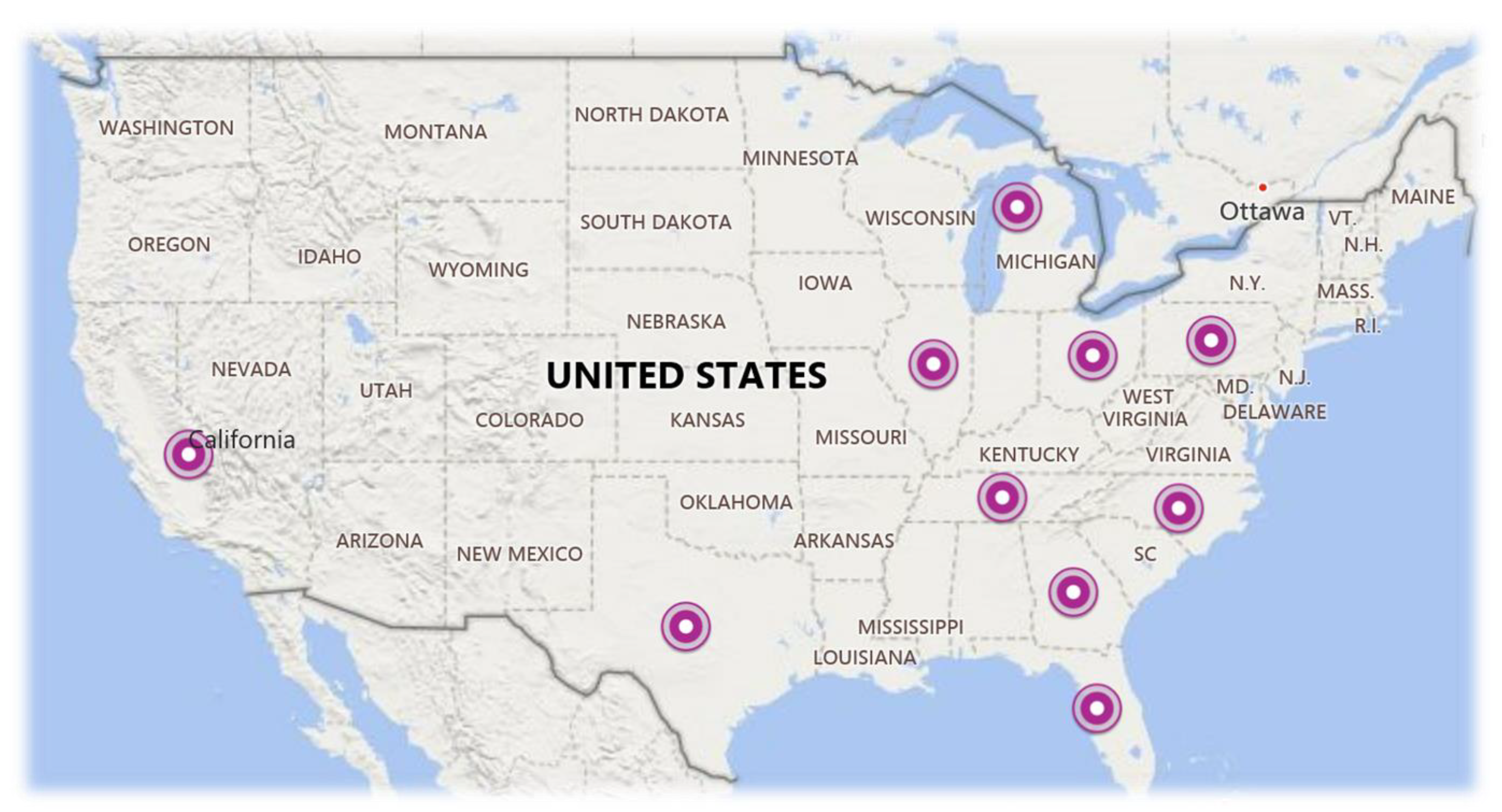
As shown in Figure 1, this study selected the top ten states in terms of crashes. These states are California, Florida, Georgia, Illinois, Michigan, North Carolina, Ohio, Pennsylvania, Tennessee, and Texas.

Figure 1.
Top Ten States in Terms of Crashes.
CART, RF, and MLP are different machine learning algorithms used in this work. Classification and Regression Trees (CART) is a machine learning algorithm that explains how the target variable’s values can be determined based on other data. It is a decision tree where each fork splits into a predictor variable, and each node ends with a prediction for the target variable. Random Forest (RF) is an ensemble learning-approach for classification, regression, and other tasks. It constructs many decision trees at training time and outputs the class, the mode of the classes (classification), or the mean estimation (regression) of the individual trees. The Multilayer Perceptron (MLP) is a feedforward ANN that generates outputs by passing input data via multiple layers of neurons. Next, what distinguishes the use of these algorithms will be explained in detail.
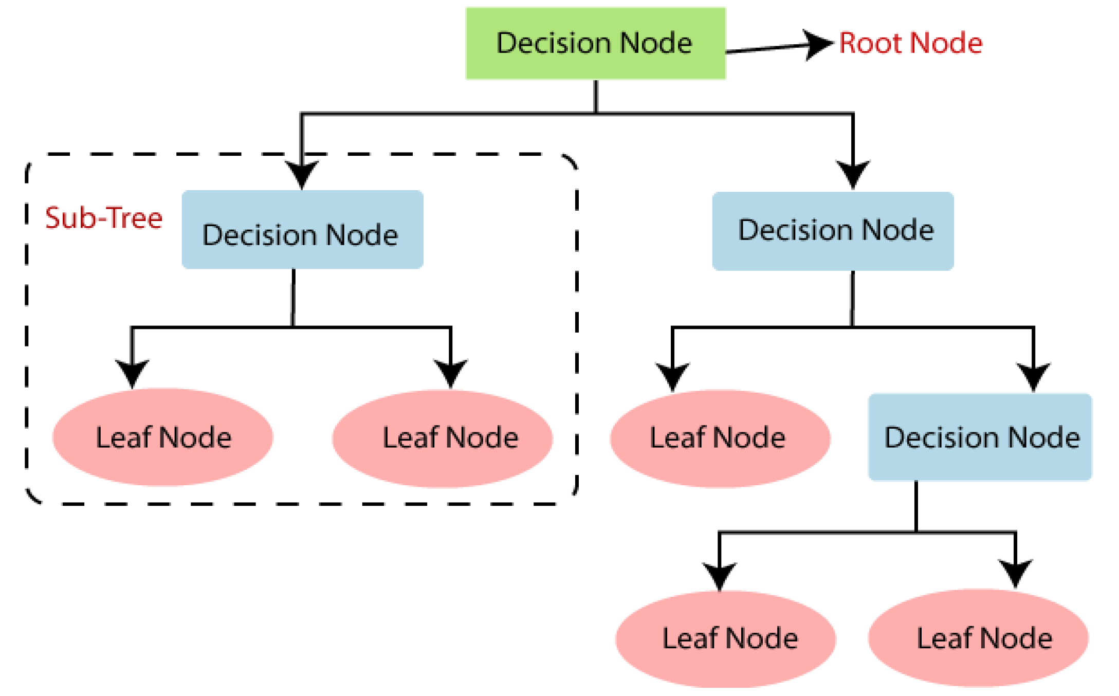
CART is one of the machine learning techniques, consisting of nodes and branches similar to a tree. It starts with the root (parent) node, which contains all the data; this node starts splitting based on a selected variable according to splitting criteria or impurity function [32]. The impurity function is a splitting criterion used to specify the suitable variable that gives the best subset at the splitting point. Entropy, Gini index, and minimum error are examples of impurity functions aiming to select the split that gives the most significant difference between the parent node’s impurity and the impurity of the weighted average of the child nodes [33]. In order to produce a tree of an appropriate size and improve model predictions, a pruning process is conducted after the training phase to remove any unimportant branches [32]. The widely used impurity function is the Gini index, which is calculated using Equation (1), where p(k|t) is the dependent variable probability equal to k at node t, and (n) is the classes number. Figure 2 shows the CART structure.

Figure 2.
CART structure [34].
RF is a regression and classification machine learning algorithm. It depends on ensemble learning, where many classifiers are combined to solve a complex problem. The RF algorithm contains many decision trees and utilizes a bootstrap aggregation or bagging technique to train the forest and improve its accuracy. The bagging technique randomly resamples the original data to create a training dataset with replacement [35]. Figure 3 shows the RF structure. The final result for RF is the average predictions for regression problems, while classification is the primary vote for individual tree predictions.
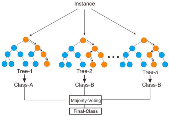
Figure 3.
RF Structure [36].
The dataset resulting from the bagging technique is divided into two parts. The first part contains about 2/3 of the dataset and is used for training the individual decision trees. The remaining (1/3 dataset) is called “out-of-bag” and is used for performance evaluation. The decision trees classify out-of-bag elements. The ratio between the misclassified samples and the out-of-bag elements represents the generalization error. The final result for RF is the average of the predictions for regression problems, while the final result for classification problems is the major vote for the predictions.
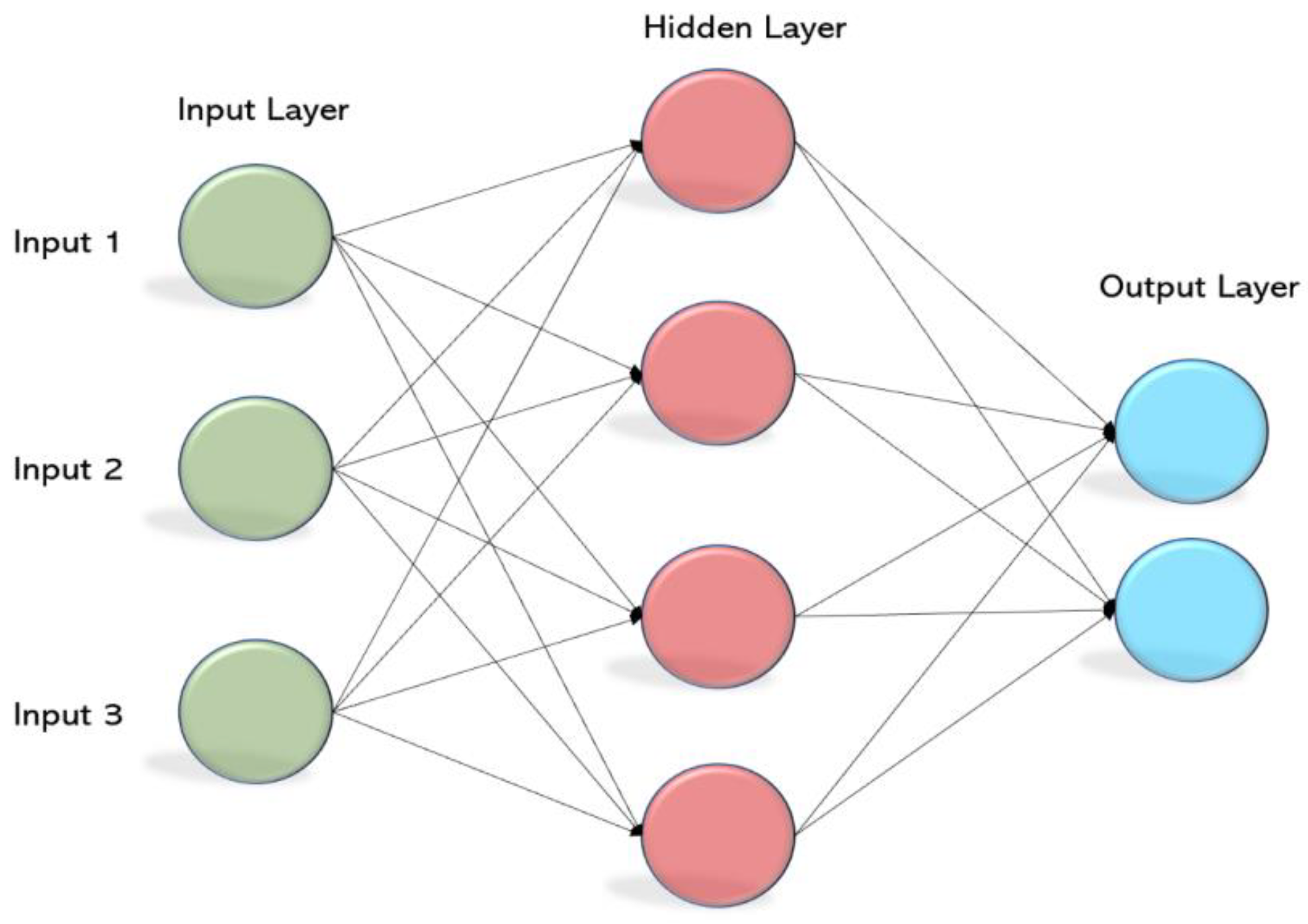
An MLP is a kind of neural network consisting of different layers (i.e., input, hidden, and output layers), and each layer contains perceptrons or nodes. The first layer is the input layer for the input variables, and the final layer is the output layer for the final result. The hidden layer is located between the input and output layers and contains the activation function. Figure 4 shows the structure of the MLP algorithm.
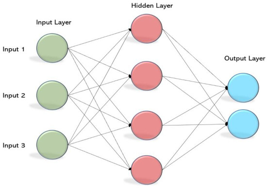
Figure 4.
MLP structure [37].
Each neuron accepts the previous layer’s output and produces the next layer’s output through the activation function. The activation or transfer function finds the node output based on the input from the previous layer [38]. MLP uses the back-propagation technique to improve model performance. It estimates the error for the predicted and correct values; this error is fed back several times to adjust the connections’ weights and produce a small error [39].
In this work, the studied dataset is imbalanced; the number of categories for the independent variable is not equal, producing a poor model. To overcome this problem, the Synthetic Minority Oversampling Technique (SMOTE) was used [40]. SMOTE is a technique used to generate new minority class records by interpolating the minority classes. It depends on selecting a random sample from the minority classes and specifying the K nearest neighbors to that sample. One of these K nearest neighbors is selected randomly to create a synthetic sample at a random point between the first selected random sample and the selected K nearest neighbor. In addition, classifiers’ performance was examined by using different evaluation metrics. These metrics are Accuracy, Root Mean Squared Error (RMSE), F-measure, Kappa statistic, Receiver Operating Characteristic (ROC) curve, and Area Under the Curve (AUC).
Accuracy is the ratio between the correct classified instances and all instances. In data science, accuracy refers to data free of errors and can be relied upon as a data source [41]. It is the first and most crucial standard/component of the data quality architecture. It is the degree to which a calculated or measured value is close to the actual value [42]. In machine learning, accuracy is a metric used for estimating classification models. It is the fraction of forecasts the model obtained right.
Accuracy = (TP + TN)/(TP + TN + FP + FN)
Accuracy can also be calculated in terms of positives and negatives, as seen below. Where:
- TP: True-positive classified instances.
- TN: True-negative classified instances.
- FP: False-positive classified instances.
- FN: False-negative classified instances.
TP, FP, TN, and FN form what is called a confusion matrix. It is a matrix used for classifier performance evaluation. It contains the actual and predicted values. Figure 5 shows the layout of the confusion matrix.
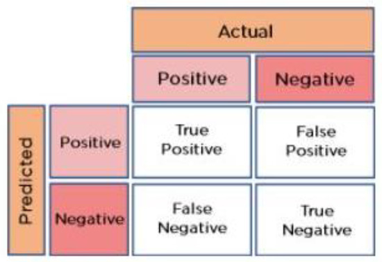
Figure 5.
Confusion Matrix [43].
- True positive is the number of times the predicted value is positive, and it is truly positive [43].
- False positive is the number of times the predicted value is positive, but it is truly negative [43].
- True negative is the number of times the predicted value is negative, and it is truly negative [43].
- False negative is the number of times the predicted value is negative, but it is truly positive [43].
RMSE measures the difference between the predicted and observed values.
where:
- RMSE: Root Mean Squared Error.
- : ith observation predicted value.
- : ith observation actual value.
- N: Observations number.
The F-measure, also called the F1-score, is used to measure model accuracy on a dataset. It is used to evaluate classification systems that classify examples as ‘positive’ or ‘negative’. The F-score integrates the precision and recall of the model. Equation (4) below for the standard F1-score is the harmonic mean for the precision and recall of the model [44].
Precision and recall are two ways to measure how well a classifier works in binary and multiclass classification problems. Precision is calculated by dividing the number of true positives by the sum of true positives and false positives. Recall, in comparison, is the ratio of instances that were correctly classified (True Positives) to the total number of instances that should have been classified as Positive (True Positives + False Negatives) [42]. Where: Precision = TP/(TP + FP), and Recall = TP/(TP + FN).
Kappa statistic is a measure of how close the classified instances are to the true ones.
where:
- : Observed instances.
- : Expected instances.
ROC curve is a binary classification performance measure. It is a probability curve that plots the True Positive Rate (TPR) against the False Positive Rate (FPR) at various threshold values. The area under the ROC curve indicates a test’s overall classification ability. The AUC measures a classifier’s ability to distinguish between classes and is used to summarize the Receiver Operating Characteristic (ROC) curve. The greater the AUC, the more accurate the model, discriminating between positive and negative classes.
3. Results
Evaluating machine learning models and algorithms is crucial to any research or project. The quality of a statistical or machine-learning model is measured using evaluation metrics. To examine the classifiers’ performance and specify the best one, the evaluation metrics were utilized to compare the classifiers’ performance. Table 2 shows the four-evaluation metrics: accuracy, RMSE, Kappa statistic, and F-measure for the three classifiers.

Table 2.
Evaluation Metrics.
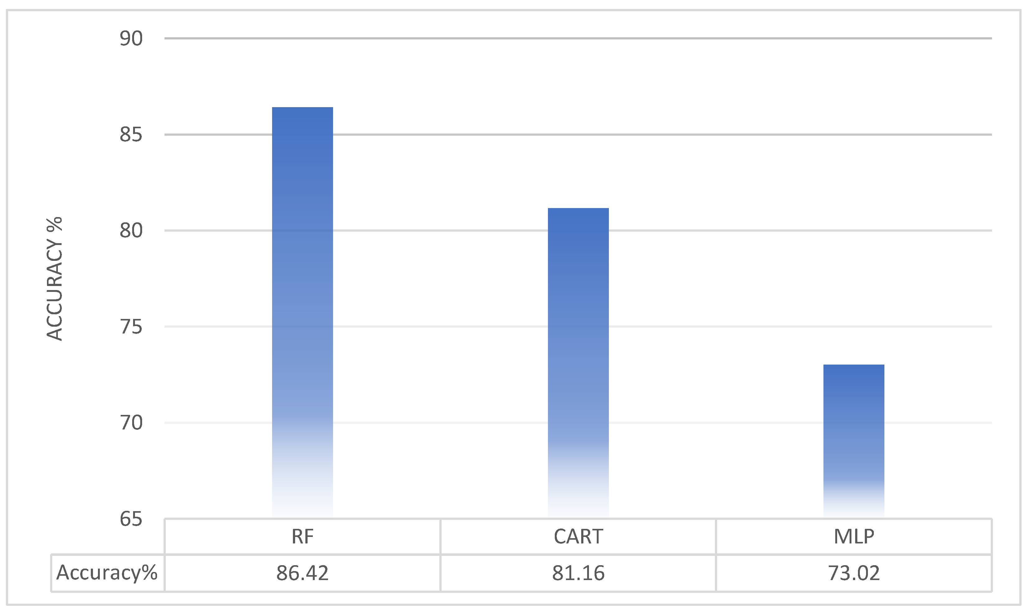
These values for RF, CART, and MLP are 86.42%, 81.16% and 73.02%, respectively. The RF achieved the highest accuracy value, while the lowest value was for the MLP algorithm. Figure 6 shows the accuracy values.
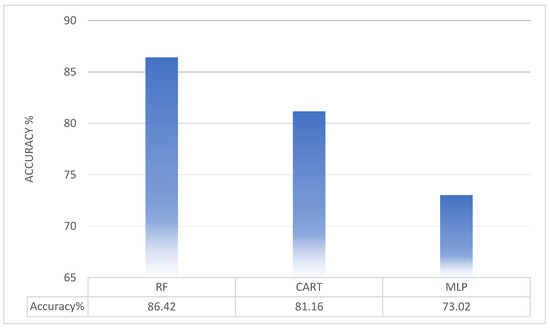
Figure 6.
Classifiers’ Accuracies.
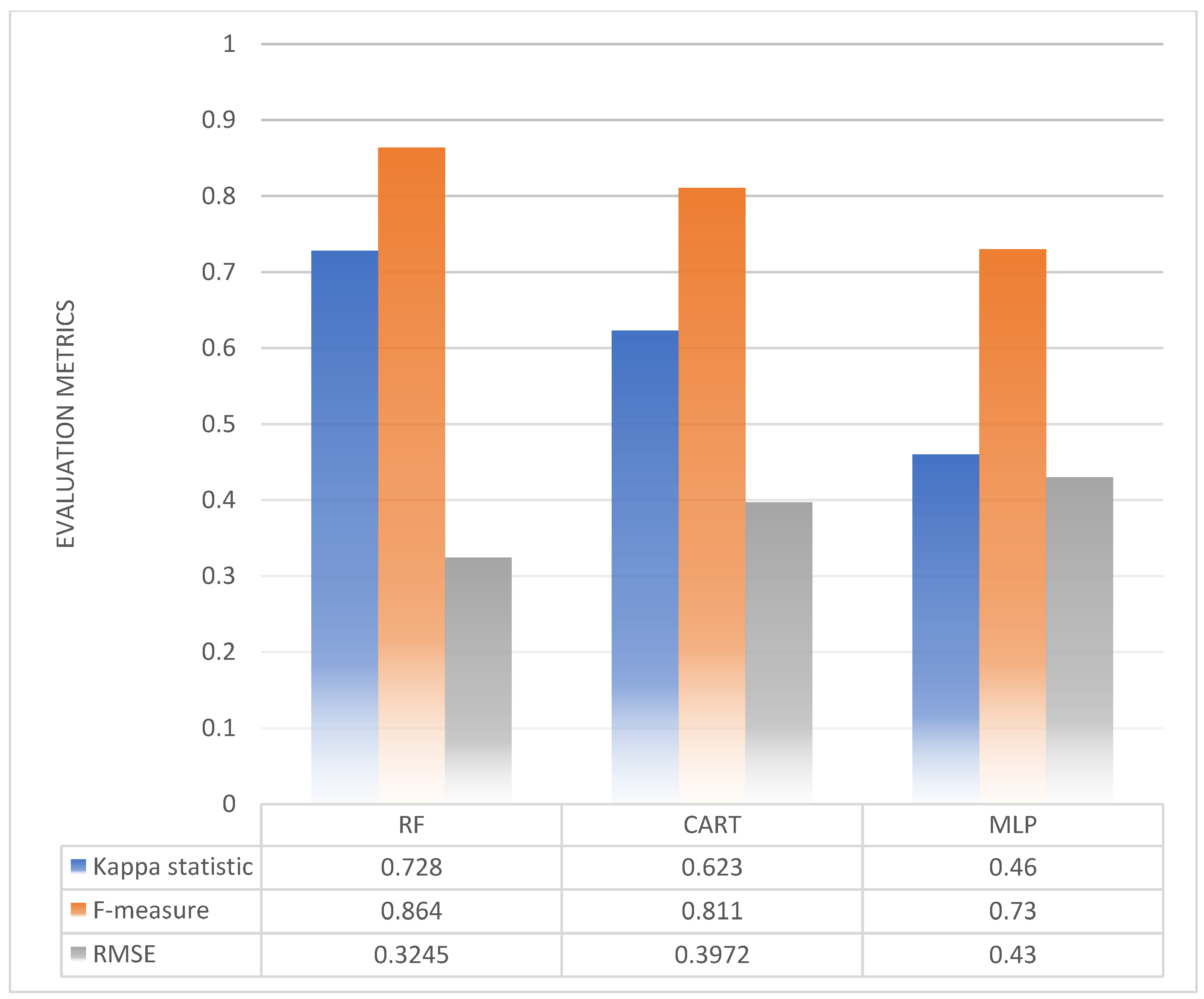
The Kappa statistic measures how close the classified instances are to the true ones. An F-measure is used to measure the model’s accuracy. Figure 7 shows the Kappa statistic, F-measure, and RMSE results. The Kappa statistic values for RF, CART, and MLP are 0.728, 0.623, and 0.46, respectively. The F-measure values for RF, CART, and MLP are 0.864, 0.811, and 0.73, respectively. Kappa statistic values for RF and CART are between 0.61 and0.8; substantial agreements, MLP Kappa statistic value is within the range (0.41–0.6); moderate agreement. F-measure values are high and indicate excellent accuracy.

Figure 7.
Kappa, F-measure, and RMES Results.
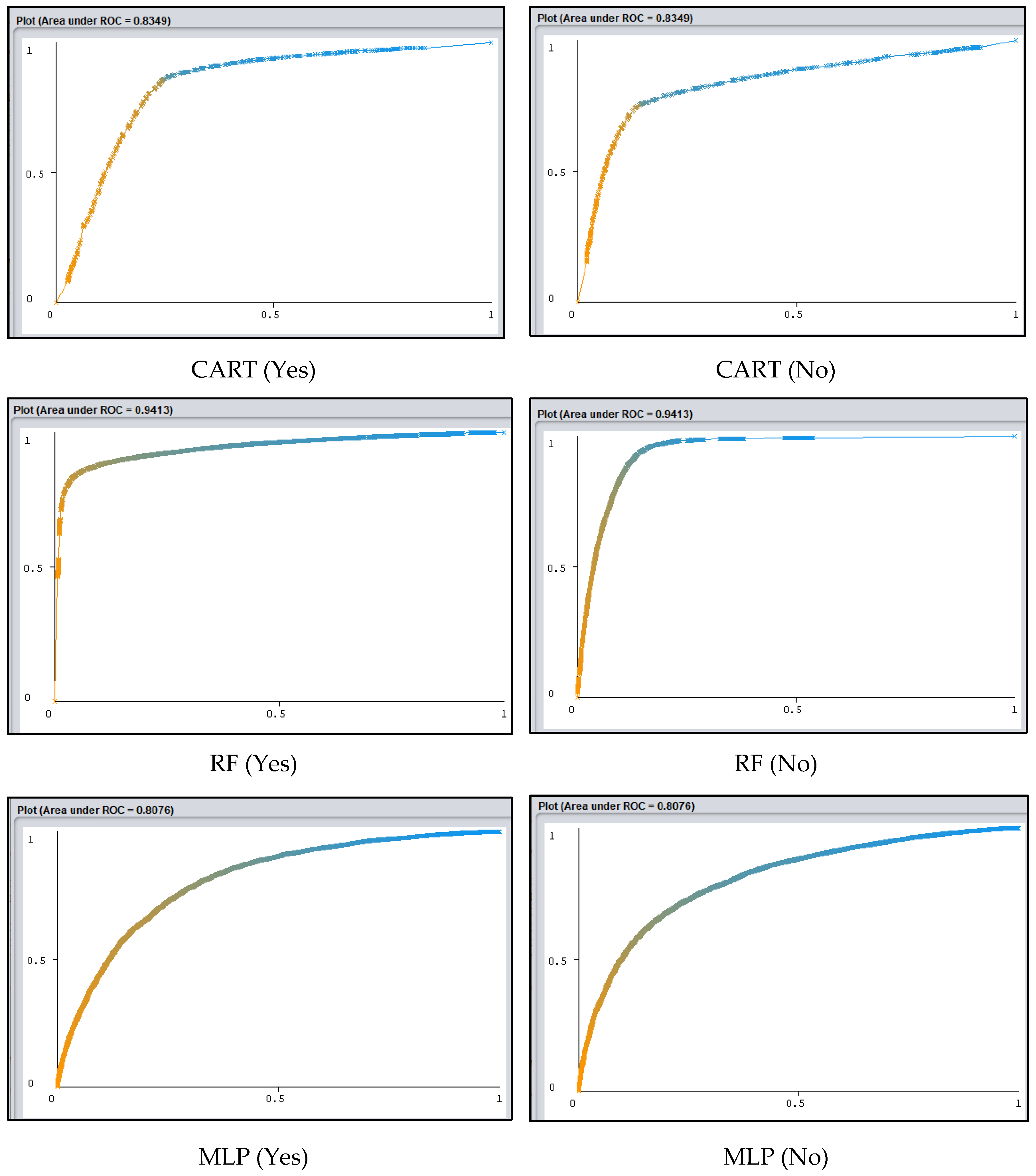
RMSE showed the error in predicting the true values. The RMSE values for RF, CART, and MLP are 0.3245, 0.3972, and 0.43, respectively. RF achieved the lowest value, while MLP achieved the highest value. AUC indicated the ability of the model to distinguish between the classes. ROC showed the relationship between the true-positive rates (Y-axis) and false-positive rates (X-axis). Table 3 presents AUC and ROC values; the results show that all the AUC values for all classifiers are more than 0.5; the classifiers have a good ability to distinguish classes. RF has the highest values, which indicate excellent performance. Figure 8 shows the ROC curves for the classifiers. The approach of the curve from the top-left corner indicates the good performance of the algorithm. It is obvious that the RF curve is the closest one to the top-left corner (i.e., it gives the best performance).

Table 3.
AUC and ROC results.
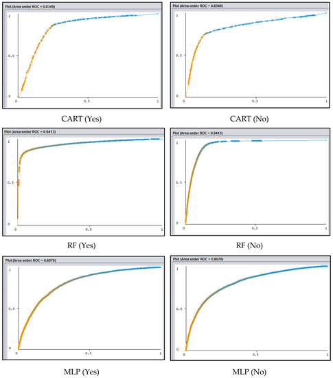
Figure 8.
ROC curves for the two classes: Yes (left figures), No (right figures).
Based on the analysis results, the three classifiers showed good ability for classifying and predicting speeding violations, especially RF. The superior performance of the RF is due to its nature. Its result depends on the majority votes for several decision trees. RF uses the bagging technique, which depends on randomness for data selection. In addition to that, there is no association between the decision trees in RF, which increase the forest accuracy. Furthermore, RF does not need many calculations to build the model and can deal with missing values, unlike the MLP.
Age, road alignment, speed limit, weather, and accident time were the most influential factors for speeding violations in this study. Age groups (≤25) and (26–35) were associated with speeding violations; this result is matched with several previous studies [17,20,21]. As well, young drivers underestimate the speeding risk and overestimate their driving abilities, so they tend to violate speed limits. This conclusion supports several previous studies [17,18,19,20,21,45,46,47]. However, Zhang et al. (2014) [18] found that age does not affect speeding violations. Another influencing factor in this study was road alignment. The results showed that speeding violations increase at curves. Different factors at curves affect vehicles’ speeds, such as the radius of the horizontal curve and the sight distance at vertical curves. Increasing the sight distance and the radius of the horizontal curve encourages driving at high speed [15,48,49,50]. The speed limit was a significant factor in this study that affected speeding violations. Different age groups violate speed limits at different speeds (30–40, 40–50, 50–60, 60–70, 70–80, and 80–90 km/h). These speed limits may not be appropriate for traffic streams. According to Gargoum et al. (2016) [13], Shawky et al. (2017) [51], and Afghari et al. (2018) [15], speeding violations decrease with increasing speed limits.
In this study, bad weather conditions (i.e., snow, ice, rain) increased speeding violations. In the winter, slippery roads because of ice, snow, or rain at low temperatures increase breaking distance, which increases the probability of speeding. These results matched those of Li et al. (2021) [52] and Ambo et al. (2021) [53]. However, Sutela and Aaltonen (2020) [54] concluded that speeding violations decreased in rainy weather. Nevertheless, another study by Zhang et al. (2014) [18] mentioned that weather conditions did not affect speeding violations. Furthermore, speeding violations were affected by accident time. In this study, night periods experienced high levels of speeding violations, which agrees with Zhang et al. (2014) [18] and Wu and Hsu (2019) [47], who said that a higher probability of speeding violations was associated with midnight and dawn periods. On the other hand, Balasubramanian and Sivasankaran (2021) [21] concluded that speeding violations were associated with daylight more than at night.
Determining the factors that affect speeding violations helps understand the violations more clearly and find the best solutions to mitigate them. In addition, using ML algorithms shows an excellent ability to analyze and predict speeding violations, which encourages using them in further studies and for similar issues.
4. Conclusions
This research aimed to analyze speeding violations in the U.S. using machine learning techniques, including CART, RF, and MLP. A total of 51,136 data records from the FARS were analyzed using WEKA software. Data related to drivers, the environment, vehicles, roads, and accident time were studied. The data were cleaned and balanced using the SMOTE technique. The accuracy, RMSE, F-measure, Kappa statistic, AUC, and ROC evaluation metrics were used to check the performance of the algorithms.
The outcome of this research concluded that young drivers tend to underestimate speeding risks and overestimate their driving abilities. Speeding violations were more common in the age groups (25) and (26–35); the percentages of violators in these two groups were 30.7% and 25.7%, respectively. Bad weather conditions were also associated with a high percentage of speeding violations. Slippery roads due to rain, snow, or ice at low temperatures increase braking distance, which raises speeding violations. The speed limit was a significant factor affecting speeding violations. Different age groups violate speed limits at different speeds (30–40, 40–50, 50–60, 60–70, 70–80, and 80–90 km/h). These speed limits may not be appropriate for traffic streams. Another influencing factor in this study was road alignment. The results showed that speeding violations increase at curves. Different factors at curves affect vehicles’ speeds, such as the radius of the horizontal curve and the sight distance at vertical curves. Furthermore, speeding violations were affected by accident time, whereby night periods experienced high speeding violations.
The analysis results indicated that the three classifiers were capable of classifying and predicting speeding violations. The RF was the best method for analyzing and predicting speeding violations. Based on the results of this study, it is recommended to raise the awareness of drivers, especially the young ones, about the dangers of excessive speed, in general, and its dangers under bad weather conditions. In addition, it is urged to apply the law firmly and fairly and increase police enforcement. This work focused on studying speeding violations, in general, using CART, RF, and MLP. For further studies, it is recommended to use different ML algorithms and utilize other programs or programming languages for studying speeding violations. Furthermore, speeding violations can be studied for more specific cases, such as speeding violations for vehicle type (i.e., passenger cars or trucks), area type (i.e., rural, or urban), or any other specific factor. Speeding violations should also be studied with traditional statistical and machine learning methods. Then, compare how well each method can predict speeding violations.
Author Contributions
Conceptualization, A.H.A. and T.K.A. Methodology, A.H.A., B.W.A.-M. and T.K.A. Software, T.K.A. and M.S.O. Validation, A.H.A., T.K.A. and M.S.O. Formal analysis, A.H.A., T.K.A. and M.S.O. Investigation, A.H.A. and T.K.A. Resources, A.H.A. and B.W.A.-M. Data curation, T.K.A. and M.S.O. Writing—original draft preparation, A.H.A. and T.K.A. Writing—review and editing, A.H.A., B.W.A.-M., T.K.A. and M.S.O. Visualization, A.H.A. and T.K.A. Supervision, A.H.A. and B.W.A.-M. Project administration, A.H.A. and B.W.A.-M. All authors have read and agreed to the published version of the manuscript.
Funding
This research received no external funding.
Institutional Review Board Statement
Not applicable.
Informed Consent Statement
Not applicable.
Data Availability Statement
This study obtained data from the Fatality Analysis Reporting System (FARS) for the years 2015–2019. The National Highway Traffic Safety Administration (NHTSA) is responsible for maintaining this database system. Available at: https://www.nhtsa.gov/research-data/fatality-analysis-reporting-system-fars (accessed on 10 January 2023).
Conflicts of Interest
The authors declare no conflict of interest. The roles in the collection, analysis, or interpretation of data; in the writing of the manuscript, and the decision to publish the results are solely by the authors.
References
- CDC. Centers for Disease Control and Prevention. Road Traffic Injuries and Deaths—A Global Problem. 2020. Available online: https://www.cdc.gov/injury/features/global-road-safety/index.html (accessed on 10 January 2023).
- Lee, N. Speed-Related Car Accidents Cost the U.S. over $40 Billion Annually. Lowering the Limit May Not Help. Consumer News and Business Channel. Available online: https://www.cnbc.com/2021/12/16/heres-why-speed-limits-arent-working-in-the-us.html (accessed on 10 January 2023).
- NHTSA. National Highway Traffic Safety Administration. Speeding|NHTSA. Available online: https://www.nhtsa.gov/risky-driving/speeding (accessed on 10 January 2023).
- Weng, J.; Meng, Q. Effects of environment, vehicle and driver characteristics on risky driving behavior at work zones. Saf. Sci. 2012, 50, 1034–1042. [Google Scholar] [CrossRef]
- Svenson, O.; Eriksson, G.; Slovic, P.; Mertz, C.K.; Fuglestad, T. Effects of main actor, outcome and affect on biased braking speed judgments. Judgm. Decis. Mak. 2012, 7, 235–243. [Google Scholar] [CrossRef]
- IIHS-HLDI Crash Testing and Highway Safety. Speed. 2021. Available online: https://www.iihs.org/topics/speed (accessed on 1 February 2022).
- WHO, World Health Organization. Road Traffic Injuries. Available online: https://www.who.int/news-room/fact-sheets/detail/road-traffic-injuries#:~:text=Key%20facts,road%20traffic%20crashes%20by%202020 (accessed on 10 January 2023).
- Sayed, T.; Abdelwahab, W.; Navin, F. Identifying accident-prone locations using fuzzy pattern recognition. J. Transp. Eng. 1995, 121, 352–358. [Google Scholar] [CrossRef]
- WHO, World Health Organization. Urban Speed Limit Range. Available online: https://www.who.int/gho/road_safety/legislation/situation_trends_urban_speed_limit/en/ (accessed on 1 February 2023).
- Alomari, A.H.; Al-Omari, B.H.; Al-Adwan, M.E.; Sandt, A. Investigating and modeling speed variability on multilane highways. Adv. Transp. Stud. 2021, 54, 5–16. [Google Scholar]
- Alomari, A.H.; Al-Omari, B.H.; Al-Adwan, M.E. Analysis of speed variance on multilane highways in Jordan. In Proceedings of the 1st International Congress on Engineering Technologies, Irbid, Jordan, 16–18 June 2020; CRC Press: Boca Raton, FL, USA, 2021; pp. 206–216. [Google Scholar] [CrossRef]
- Build, Price, Option. Top 8 Reasons Why Drivers Speed—Build, Price, Option. 2020. Available online: https://www.buildpriceoption.com/top-8-reasons-why-drivers-speed/ (accessed on 10 January 2023).
- Gargoum, S.A.; El-Basyouny, K.; Kim, A. Towards setting credible speed limits: Identifying factors that affect driver compliance on urban roads. Accid. Anal. Prev. 2016, 95, 138–148. [Google Scholar] [CrossRef]
- Kanellaidis, G.; Golias, J.; Zarifopoulos, K. A survey of drivers' attitudes toward speed limit violations. J. Saf. Res. 1995, 26, 31–40. [Google Scholar] [CrossRef]
- Afghari, A.P.; Haque, M.M.; Washington, S. Applying fractional split model to examine the effects of roadway geometric and traffic characteristics on speeding behavior. Traffic Inj. Prev. 2018, 19, 860–866. [Google Scholar] [CrossRef] [PubMed]
- Huang, Y.; Sun, D.; Tang, J. Taxi driver speeding: Who, when, where and how? A comparative study between Shanghai and New York City. Traffic Inj. Prev. 2018, 19, 311–316. [Google Scholar] [CrossRef]
- Tseng, C.M. Speeding violations related to a driver’s social-economic demographics and the most frequent driving purpose in Taiwan’s male population. Saf. Sci. 2013, 57, 236–242. [Google Scholar] [CrossRef]
- Zhang, G.; Yau, K.K.; Gong, X. Traffic violations in Guangdong Province of China: Speeding and drunk driving. Accid. Anal. Prev. 2014, 64, 30–40. [Google Scholar] [CrossRef]
- Liang, Z.; Xiao, Y. Analysis of factors influencing expressway speeding behavior in China. PLoS ONE 2020, 15, e0238359. [Google Scholar] [CrossRef]
- Al Matawaha, J.; Jadaan, K.; Freeman, B. Analysis of speed related behavior of Kuwaiti drivers using the driver behavior questionnaire. Period. Polytech. Transp. Eng. 2020, 48, 150–158. [Google Scholar] [CrossRef]
- Balasubramanian, V.; Sivasankaran, S. Analysis of factors associated with exceeding lawful speed traffic violations in Indian metropolitan city. J. Transp. Saf. Secur. 2021, 13, 206–222. [Google Scholar] [CrossRef]
- Al-Mistarehi, B.W.; Alomari, A.H.; Imam, R.; Alnaasan, T.K. Investigating the Factors Affecting Speeding Violations in Jordan Using Phone Camera, Radar, and Machine Learning. Front. Built Environ. 2022, 8, 917017. [Google Scholar] [CrossRef]
- Mohammadazadeh, A.; Sabzalian, M.H.; Castillo, O.; Sakthivel, R.; El-Sousy, F.F.; Mobayen, S. Neural Networks and Learning Algorithms in MATLAB; Springer Nature: Berlin/Heidelberg, Germany, 2022. [Google Scholar]
- Mohammadzadeh, A.; Sabzalian, M.H.; Zhang, C.; Castillo, O.; Sakthivel, R.; El-Sousy, F.F. Modern Adaptive Fuzzy Control Systems (Vol. 421); Springer Nature: Berlin/Heidelberg, Germany, 2022. [Google Scholar]
- Alomari, A.H.; Khedaywi, T.S.; Jadah, A.A.; Marian, A.R.O. Evaluation of Public Transport among University Commuters in Rural Areas. Sustainability 2023, 15, 312. [Google Scholar] [CrossRef]
- Alomari, A.H.; Khedaywi, T.S.; Marian, A.R.O.; Jadah, A.A. Traffic speed prediction techniques in urban environments. Heliyon 2022, 8, e11847. [Google Scholar] [CrossRef]
- Alomari, A.H.; Abu Lebdeh, E. Smart real-time vehicle detection and tracking system using road surveillance cameras. J. Transp. Eng. Part A Syst. 2022, 148, 04022076. [Google Scholar] [CrossRef]
- Al-Mistarehi, B.W.; Alomari, A.H.; Imam, R.; Mashaqba, M. Using machine learning models to forecast severity level of traffic crashes by r studio and arcgis. Front. Built Environ. 2022, 16648714, 31. [Google Scholar] [CrossRef]
- NHTSA, National Highway Traffic Safety Administration. Fatality Analysis Reporting System (FARS). Available online: https://www.nhtsa.gov/research-data/fatality-analysis-reporting-system-fars (accessed on 10 January 2023).
- Aljarrah, M.F.; Khasawneh, M.A.; Al-Omari, A.A. Investigating Key Factors Influencing the Severity of Drivers Injuries in Car Crashes Using Supervised Machine Learning Techniques. J. Eng. Sci. Technol. Rev. 2019, 12, 15–27. [Google Scholar] [CrossRef]
- Witten, I.; Frank, E.; Hall, M.; Pal, C. The WEKA Workbench. In Data Mining: Practical Machine Learning Tools and Techniques, 4th ed.; Morgan Kaufmann: Burlington, MA, USA, 2016. [Google Scholar]
- Loh, W.Y. Classification and regression trees. Wiley Interdiscip. Rev. Data Min. Knowl. Discov. 2011, 1, 14–23. [Google Scholar] [CrossRef]
- Kingsford, C.; Salzberg, S. What are decision trees? Nat. Biotechnol. 2008, 26, 1011–1013. [Google Scholar] [CrossRef]
- Ampadu, H. Decision Trees. 2021. Available online: https://ai-pool.com/a/s/decision-trees (accessed on 25 December 2022).
- Breiman, L. Random forests. Mach. Learn. 2001, 45, 5–32. [Google Scholar] [CrossRef]
- Nasution, A.K.; Wijaya, S.H.; Gao, P.; Islam, R.M.; Huang, M.; Ono, N.; Kanaya, S.; Altaf-Ul-Amin, M. Prediction of Potential Natural Antibiotics Plants Based on Jamu Formula Using Random Forest Classifier. Antibiotics 2022, 11, 1199. [Google Scholar] [CrossRef]
- Mohanty, A. Multi-Layer Perceptron (MLP) Models on Real World Banking Data. Available online: https://becominghuman.ai/multi-layer-perceptron-mlp-models-on-real-world-banking-data-f6dd3d7e998f (accessed on 10 January 2023).
- Noriega, L. Multilayer Perceptron Tutorial. School of Computing. Ph.D. Thesis, Staffordshire University, Stoke-on-Trent, UK, 2005. [Google Scholar]
- Almeida, L.B. Multilayer perceptrons. In Handbook of Neural Computation C; Elsevier: Amsterdam, The Netherlands, 1997. [Google Scholar] [CrossRef]
- Chawla, N.; Bowyer, K.; Hall, L.; Kegelmeyer, W. SMOTE. Synthetic Minority Over-sampling Technique. J. Artif. Intell. Res. 2002, 16, 321–357. [Google Scholar] [CrossRef]
- What is Data Accuracy, Why it Matters and How Companies Can Ensure They Have Accurate Data. 2020. Available online: https://dataladder.com/what-is-data-accuracy/ (accessed on 8 April 2023).
- Towards Data Science. Accuracy, Recall, Precision, F-Score & Specificity, Which to Optimize on? 2019. Available online: https://towardsdatascience.com/accuracy-recall-precision-f-score-specificity-which-to-optimize-on-867d3f11124 (accessed on 8 April 2023).
- What is a Confusion Matrix in Machine Learning? 2023. Available online: https://www.simplilearn.com/tutorials/machine-learning-tutorial/confusion-matrix-machine-learning#:~:text=A%20confusion%20matrix%20presents%20a,actual%20values%20of%20a%20classifier (accessed on 8 April 2023).
- DeepAI. What Is the F-Score? 2023. Available online: https://deepai.org/machine-learning-glossary-and-terms/f-score (accessed on 8 April 2023).
- Zamanov, M.S. Development of a Prediction Model for Speed Limit Violations on Tangent Road Sections. Master’s Thesis, Delft University of Technology, Delft, The Netherlands, 2012. [Google Scholar]
- Javid, M.A.; Al-Roushdi, A.F.A. Causal factors of driver’s speeding behaviour, a case study in Oman: Role of norms, personality, and exposure aspects. Int. J. Civ. Eng. 2019, 17, 1409–1419. [Google Scholar] [CrossRef]
- Wu, Y.W.; Hsu, T.P. Mining characteristics of speeding and red-light running violations using association rules. J. East. Asia Soc. Transp. Stud. 2019, 13, 2111–2125. [Google Scholar]
- Vos, J.; Farah, H.; Hagenzieker, M. How do Dutch drivers perceive horizontal curves on freeway interchanges and which cues influence their speed choice? IATSS Res. 2021, 45, 258–266. [Google Scholar] [CrossRef]
- Poe, C.; Tarris, J.; Mason, J. Operating speed approach to geometric design of low-speed urban streets. Transp. Res. Circ. 1998, 10, 1–9. [Google Scholar]
- Fitzpatrick, K.; Carlson, P.; Brewer, M.; Wooldridge, M. Design Factors That Affect Driver Speed on Suburban Streets. Transp. Res. Rec.: J. Transp. Res. Board 2001, 1751, 18–25. [Google Scholar] [CrossRef]
- Shawky, M.; Sahnoon, I.; Al-Zaidy, A. Predicting speed-related traffic violations on rural highways. In Proceedings of the 2nd World Congress on Civil, Structural, and Environmental Engineering (CSEE’17), Barcelona, Spain, 2–4 April 2017; Volume 117. [Google Scholar] [CrossRef]
- Li, Y.; Li, M.; Yuan, J.; Lu, J.; Abdel-Aty, M. Analysis and prediction of intersection traffic violations using automated enforcement system data. Accid. Anal. Prev. 2021, 162, 106422. [Google Scholar] [CrossRef]
- Ambo, T.B.; Ma, J.; Fu, C. Investigating influence factors of traffic violation using multinomial logit method. Int. J. Inj. Control. Saf. Promot. 2021, 28, 78–85. [Google Scholar] [CrossRef] [PubMed]
- Sutela, M.; Aaltonen, M. Effects of temporal characteristics and weather conditions on speeding sanction rates in automatic traffic enforcement. Police J. 2021, 94, 590–615. [Google Scholar] [CrossRef]
Disclaimer/Publisher’s Note: The statements, opinions and data contained in all publications are solely those of the individual author(s) and contributor(s) and not of MDPI and/or the editor(s). MDPI and/or the editor(s) disclaim responsibility for any injury to people or property resulting from any ideas, methods, instructions or products referred to in the content. |
© 2023 by the authors. Licensee MDPI, Basel, Switzerland. This article is an open access article distributed under the terms and conditions of the Creative Commons Attribution (CC BY) license (https://creativecommons.org/licenses/by/4.0/).

