Article

An InSAR Interference Fringe-Matching Algorithm Based on Mountain Branch Points

1
National Key Laboratory of Microwave Imaging Technology, Aerospace Information Research Institute, Chinese Academy of Sciences, Beijing 100190, China
2
School of Electronic, Electrical and Communication Engineering, University of Chinese Academy of Sciences, Beijing 100049, China
3
Northern Institute of Technology in Electronic Equipment, Beijing 100191, China
*
Author to whom correspondence should be addressed.
Appl. Sci. 2023, 13(6), 3941; https://doi.org/10.3390/app13063941
Submission received: 16 February 2023 / Revised: 16 March 2023 / Accepted: 16 March 2023 / Published: 20 March 2023
(This article belongs to the Section Electrical, Electronics and Communications Engineering)

Abstract

:
Interferometric synthetic aperture radar (InSAR) is an integrated navigation technique that can be used for aircraft positioning and attitude retrieval, regardless of weather conditions. The key aspect of the entire system is interference fringe matching, which has not been extensively researched in existing literature. To address this gap, this paper proposes a terrain-feature-based interference fringe-matching algorithm. The proposed algorithm first extracts mountain line features from the interference fringes and identifies mountain branch points as key points for feature matching. A threshold is set to eliminate false detections of mountain branch points caused by phase mutation. Matching is then carried out by combining the mountain line features and curvature design feature descriptors of the area around a branch point. The proposed algorithm is verified using interference fringe data obtained from an actual flight experiment in Inner Mongolia, China, compared to a reference interference fringe dataset with errors. The results show that, under the condition of position error, the proposed algorithm yields 72 matching inliers with a precision of 0.103, a recall of 0.128, and an F1-Score of 0.144. Compared to traditional algorithms, our proposed algorithm significantly improves the problem of mismatch and opens up new possibilities for downstream interference fringe matching navigation technology. Furthermore, the proposed algorithm provides a new approach for remote sensing image matching using terrain features.

1. Introduction

As modern society continues to develop, the demand for precise aircraft navigation is increasing. Therefore, studying high-precision and highly autonomous navigation systems has become increasingly important [1]. An inertial navigation system (INS) is a vital component of combined navigation systems due to its short-term stability and the fact that is does not require an exchange of information with the outside world. Therefore, a combination of other navigation methods is needed to correct the accumulation of INS errors and achieve accurate navigation [2]. This is the case with the existing combined navigation systems. There are many problems with existing combined navigation systems: optical image-matching-based scene-aided navigation systems do not have all-weather capability and are heavily influenced by seasons [3]; synthetic aperture radar (SAR) scene-matching navigation systems cannot achieve accurate three-dimensional positioning [4]; terrain-matching navigation systems do not have cross-course resolution and have low navigation accuracy [5], and global positioning system (GPS)-aided navigation systems rely on satellite signals and cannot achieve autonomous navigation [6].
Interferometric synthetic aperture radar has an inherent advantage in both acquiring images of the observed area and inverting high-precision digital terrain due to its imaging mechanism [7]. The authors of [8] proposed the use of interference fringes that can be generated in real time and with terrain information to achieve matched navigation, and others have performed further research [9,10]. The InSAR interference fringe-matching navigation system is shown in Figure 1 [10], where the airborne InSAR system first acquires echo data and the INS outputs navigation data for self-aligned imaging, which is used to generate interference fringes in real time; the DEM database then generates reference interference fringes in real time according to the reference trajectory and system parameters output by the system, and the actual acquired interference fringes are matched with the reference interference fringe to extract the position of the eponymous point. At the same time, the platform motion parameters are estimated based on the time-varying baseline, Doppler frequency, point-target phase history and other coherent data of the InSAR system. Finally, the unified InSAR observation and observation error equations are constructed by combining the results of motion parameter estimation with those of interference fringe-matching positioning, and combined filtering with INS is used to correct the accumulated drift errors and output the combined navigation parameters. Compared with matched navigation systems based on DEM data, interference fringe data are more sensitive to aircraft attitude [11,12] and have greater potential.
The entire system requires a high degree of accuracy in the interference fringe-matching algorithm, which directly impacts the accurate output of subsequent navigation parameters. However, the interference fringe-matching algorithm is a challenging area of research. Several researchers [8,9,10,11] have made important contributions to the framework of matching navigation with interference fringes but have not conducted in-depth studies of the interference fringe-matching algorithm and only used traditional matching algorithms to complete the task of matching. SIFT [13], as a representative traditional matching algorithm, uses Gaussian pyramids to detect keypoints, uses gradient information around the keypoints for description, is invariant to both rotation and scale, and has good robustness to noise and changes in viewpoint and illumination. SURF [14] is an improvement of SIFT based on the use of integral maps and wavelet responses, which are faster and more robust. The ORB [15] algorithm is a method for extracting image features that is based on the features from the accelerated segment test (FAST) [16] keypoint detector and the binary robust independent elementary features (BRIEF) [17] descriptor. Although the ORB algorithm is more efficient than SURF and can process larger images, its matching accuracy is low. In recent years, there have been some related improved algorithms [18,19,20]. However, those algorithms all start from feature point detection, which does not take into account the rich terrain information contained in the interference fringes, and when the vehicle flies over a large area of mountains, those algorithms are less effective in matching the texture features between different mountains, due to their similarity. With the advancement of deep learning, its applications in image matching are endless. In 2015, Koch et al. [21] proposed a single sample image recognition method based on twin neural networks. This method utilizes two convolutional neural networks with shared parameters to extract image features and calculates similarity using Euclidean distance. Lift [22] can learn the invariance features in the image and convert them into descriptors that can be used for matching and retrieval. In recent years, achievements such as SuperPoint [23] and Superglue [24] have also demonstrated the potential of deep learning in the field of image matching. However, the interference fringe is a special data source, and there is no large public dataset available for training. Models trained on ordinary optical datasets are not effective in the interference fringe matching task. An interferometric fringe registration algorithm has been integrated into common InSAR processing software [25,26]. This algorithm first simulates a pair of SAR intensity images from DEM data and then uses the simulated images for registration with the real SAR intensity images, thus completing the registration of corresponding interference fringes. However, when an aircraft has attitude errors, these different attitude errors correspond to the same DEM data, with the result that the registration results of interference fringes do not change with the changes in errors. Therefore, it is necessary to develop an effective algorithm that can directly match the interference fringes. However, there is no research on direct matching of interference fringe data, so in this study, we make full use of the topographic information contained in interference fringes and propose a method for matching interference fringes based on mountain branch points. The algorithm was first designed to extract the mountain range line features, detect mountain range branch points on the basis of online features, design feature descriptors in conjunction with mountain range line features and curvatures in the areas around the branch points, and match at Euclidean distances, improving the matching performance of interference fringes compared with conventional algorithms through the use of measured data. The primary focus of this paper is on the matching task of interference fringes, and the research encompasses the following key contributions:
  • An analysis is conducted of the correspondence between the interference fringes and the DEM to design an algorithm for the extraction of mountain range lines from the interference fringes;
  • The use of mountain range branch points is proposed as a keypoint for feature matching, which is a new idea for image matching of topographic data such as interference fringes and DEM;
  • Improved matching of interference fringes is achieved by designing more specific feature descriptors for mountain branch points.

2. Methods

2.1. Algorithm Flow

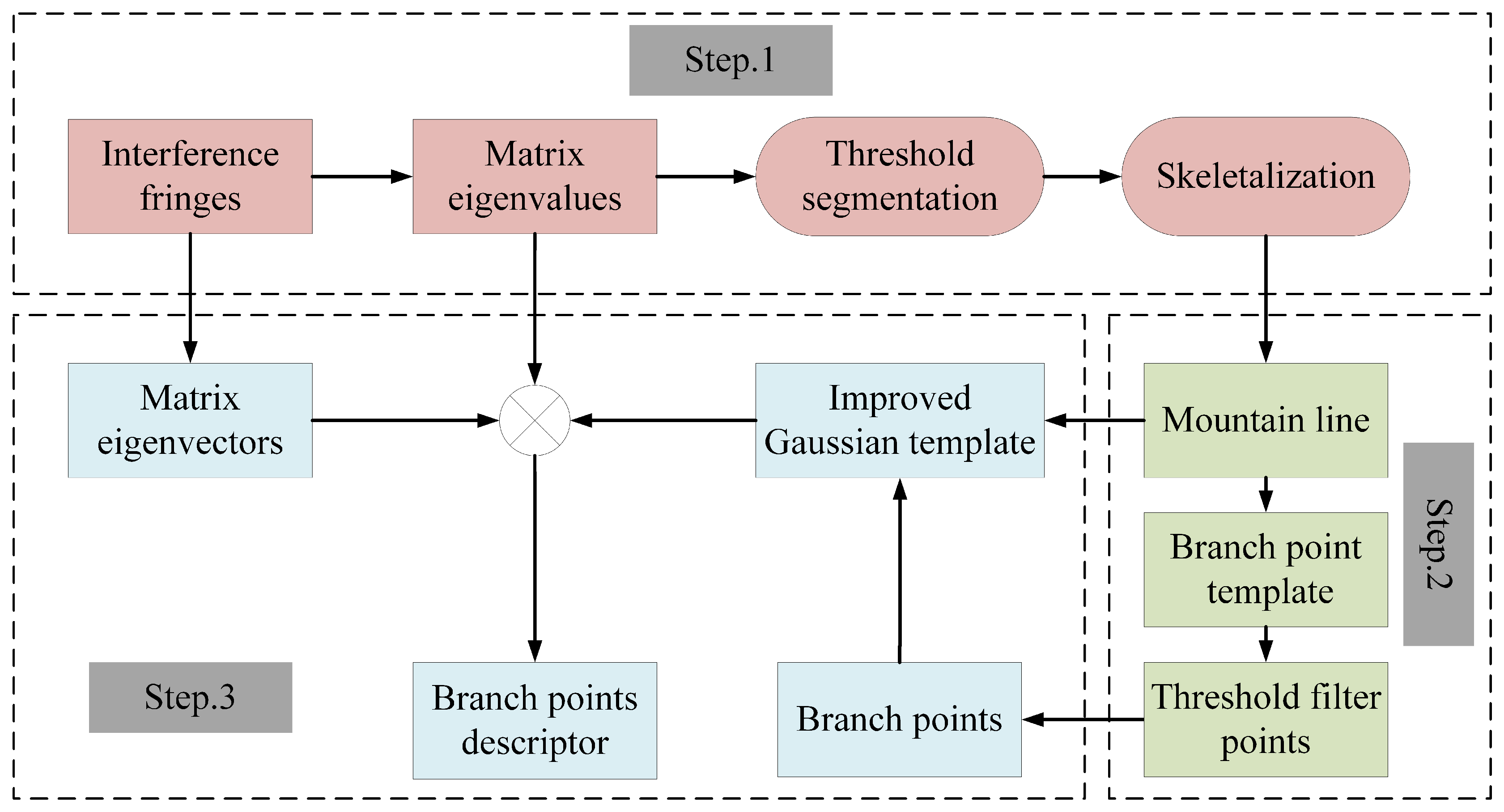
As analyzed in Section 1, the primary reason why traditional algorithms cannot effectively match interference fringes is that they fail to utilize the abundant terrain features present within the interference fringes. Therefore, based on this point, this paper first designs an algorithm to extract the mountain line features contained in interference fringes, and then the mountain branch points are detected based on online features, such as the keypoints, for feature matching; this matching is carried out by combining the mountain line features and curvature design feature descriptors of the area around a branch point. The algorithm for matching the interference fringes proposed in this paper is shown in Figure 2. The first step is to calculate the Hessian matrix of interference fringes and obtain the eigenvalues and eigenvectors of this matrix, set two segmentation thresholds for the eigenvalue map, one large and one small, and skeletonize on the coarse mountain range lines after threshold segmentation to obtain ridge and valley lines. In the second step, we use the branch point template to traverse the mountain ridge and obtain the mountain branch point as the key feature for image matching. To eliminate false detections caused by phase mutations, we set a threshold. In the third step, the Gaussian function is refined based on the mountain range line mask in the region around a branch point, and the descriptors are generated by assigning the direction of the descriptors from the branch point eigenvectors and obtaining a histogram of the curvature of the region around the branch point based on the eigenvalues of the pixels around the branch point. Subsequently, the branch point descriptors obtained from the two interference fringes are matched using feature descriptors at Euclidean distance according to the flow of the conventional image matching algorithm. Using the RANSAC [27] algorithm to filter out the correctly matched feature points, the navigation parameters can subsequently be output.

2.2. Interference Fringe Characterization

Figure 3a shows the geometric schematic diagram of InSAR. B is the length between antennas A 1 and A 2 or, in other words, the baseline length. H is the aircraft flight height, α is the baseline inclination angle, h is the elevation value of ground point P, θ is the downward viewing angle, R is the squint distance between antenna A 1 and P, and R + Δ R is the squint distance between antenna A 2 and P. According to the InSAR geometric schematic diagram in Figure 3a and the cosine theorem, triangle Δ A 1 A 2 P has the following relations:
( R + Δ R ) 2 = R 2 + B 2 2 R B sin ( θ α )
In practice, B is much larger than R, and R + Δ R is much larger than R. Therefore, Equation (1) can be rewritten as follows:
B sin ( θ α ) = B 2 2 R Δ R 2 2 R 2 R Δ R
According to the principle of generating DEM products by the InSAR system [28], the interference phase Δ ϕ can be expressed as Equation (3), where λ is the wavelength.
Δ ϕ = 4 π Δ R λ
According to the geometric relationship in Figure 3a, the downward viewing angle can be obtained:
θ = α arcsin λ Δ ϕ 4 π B
The elevation value h of point P is:
h = H R cos θ
The following can be obtained through simultaneous calculation of Equations (1)–(5):
Δ ϕ = 4 π B λ sin ( α cos ( H h R ) α )
According to the simulation parameters in Equation (6) and Table 1, the relationship between the ground elevation value error and the interference phase error is simulated as shown in Figure 3b.
The elevation value error of 5 m causes a 46 . 95 interference phase change, which is monotonic, so that the phase values of the interference fringes also express the rich topographic information contained in the DEM data. Topographic relief features are not specific to a single isolated pixel point but are a regional feature [29]. Traditional matching algorithms, such as SIFT and SURF, extract feature points based mainly on the texture gradient of the image and independently of the terrain orientation. The high degree of similarity between mountains leads to the traditional matching algorithm not being sufficiently effective to meet the requirements. Since the topographic features of the interference fringes are mainly embedded in the mountain range line features as in the DEM data [30], in this study, an algorithm is designed for matching the interference fringes based on this point.

2.3. Extraction of Mountain Line

A monotonic relationship exists between the DEM and the interference fringes, allowing for the design of an interference fringe mountain range line extraction algorithm based on DEM mountain range line extraction [31,32]. Edge detection is a common means for detecting line features in images. The main principle is to find the first-order derivative or gradient [33]. However, the gradient method allows only detecting boundaries with high and low phase values in interference fringe images and not those positioned directly in phase extremity regions. Figure 4a gives the function curve for the first-order derivative of a continuous function with a high value. The first-order derivative is not located directly at the high value of the function but rather in the region on either side of the high value of the function. In the interference fringe image, the lines of the mountain ranges we are interested in are represented as a collection of points with very large and very small phase values, the physical significance of which represents ridges and valleys, respectively. In the field of digital image processing, the detection of such thin lines that are darker or brighter than the surrounding area is defined as ridge detection [34]. Ridge detection usually involves finding the first-order derivative over the zero point, or second-order derivative, for the image. Figure 4a similarly shows the function curve for the second-order derivative of a continuous function, and it can be seen that the extreme values of the second-order derivative of the function correspond to where the extreme values of the original function occur. Figure 4b simulates a ridge with a bright line, and Figure 4c,d show the effect after taking the first- and second-order derivatives of the image, respectively. The first-order derivatives are presented as two bright columns distributed on either side of the true ridge position. The bright line of the second-order derivative coincides with the original ridge at its location. The second-order derivative is the tool that provides the basis for the extraction of mountain range line features for interference fringes.
In an interference fringe image, the ridge and valley lines correspond to the set of very large and very small phase value points, respectively, which also represent the curvature extrema of the surface on which the point is located. For a discrete two-dimensional digital image I, the curvature of a point p ( x , y ) on the image can be represented by a Hessian matrix [35]:
H = L x x L x y L y x L y y
L x x , L x y , L y x , L y y represent the second-order derivatives of the point. Considering that digital images inevitably have noise points, the second-order derivative of the image can be obtained by convolving the original image with a Gaussian function G ( α , β , δ ) having scale δ , as in Equation (8), where α , β denote the combination of the derivatives of x , y . Thus, a certain amount of noise can be filtered while acquiring the derivative of the image.
L α β = p ( x , y ) G ( α , β , δ ) L α β { L x x , L x y , L y x , L y y } G ( α , β , δ ) = 1 2 π δ 2 e ( α 2 + β 2 ) 2 δ 2
After defining the Hessian matrix, let the larger absolute value of its eigenvalue be u and the corresponding eigenvector be v. If u is positive, then it corresponds to the valley line in the interference fringe image, and if it is negative, then it corresponds to the ridge line in the interference fringe image. Typically, the ridge lines and valley lines obtained from the above operation are still of a certain width, and some subsequent processing is required to obtain a line feature with a pixel width of 1. The eigenvalue is obtained for each point of the image according to Equations (7) and (8). The magnitude of the eigenvalue represents the magnitude of the point curvature, and this value is independent of the magnitude of the phase value of the interference fringe, so the whole eigenvalue map of the interference fringe can be considered normalized. Then, global threshold segmentation can be used to filter out the points with high eigenvalues. The specific approach is to set a positive and a negative threshold, representing the ridge threshold T r i d g e and valley threshold T v a l l e y , respectively, and use these two thresholds to determine the ridge lines and valley lines. If the feature value is greater than T r i d g e , it can be identified as part of the ridge line. If the feature value is less than T v a l l e y , it can be identified as part of the valley line. Since this is a global threshold, the ridge lines and valley lines of the entire interference fringe can be directly detected. After thresholding, the image is binary. To obtain a line feature with a pixel width of 1, skeletonization of the image after thresholding is required. Since the introduction of the concept of skeletonization in the literature [36], a couple of different improved algorithms have been reported [37,38]. In principle, both seek a center line within a line of pixel width greater than 1. The center line remains equidistant from the two boundaries, thus preserving the basic form of the object.
The mountain range line feature extraction method for interference fringes is summarized in Figure 5. The Hessian matrix of the interference fringe is first found using Equation (7), with (8) used to calculate the corresponding eigenvalues. The eigenvalues are judged using the threshold segmentation method; values greater than the ridge line threshold T r i d g e are identified as a rough estimate of the ridge line, and values less than the valley line threshold T v a l l e y are identified as a rough estimate of the valley line. The skeletonization operation is performed on them to obtain the ridge line as well as the valley line with a pixel width of 1. These feature maps are binarized images. Figure 6a shows a demonstration area of interference fringes with a large number of ridges as well as valleys. The above detection algorithm is used for mountain range line extraction, where T v a l l e y is set to −0.7 and T r i d g e is set to 0.7. Since the scale of the real and reference interference fringes is the same, the scale of the Gaussian function δ is uniformly set to 2. The extraction results are shown in Figure 6b, where the blue lines indicate the extracted valley lines and the yellow lines indicate the extracted ridge lines. The mountain range line features implied by the interference fringes can be accurately detected.

2.4. Extraction of Mountain Branch Points

To accomplish the image matching task that follows, it is necessary to convert the extracted mountain range line features into point features. As shown in Figure 6b, the mountain range line features have multiple branches within each line. These branch points correspond to the bifurcation points of the real mountain range and indicate that the topography of the real mountain range changes at that point. Branch points with different distributions represent different topographic features, while interference fringes for the same mountain region always extract the same mountain branch points. Therefore, the interference fringes obtained in real time correspond to the branch points of the mountain range extracted from the interference fringes in the inversion of the base terrain library. Compared with the keypoints extracted using traditional matching algorithms, these branch points are highly specific and are used as feature points for subsequent image matching.
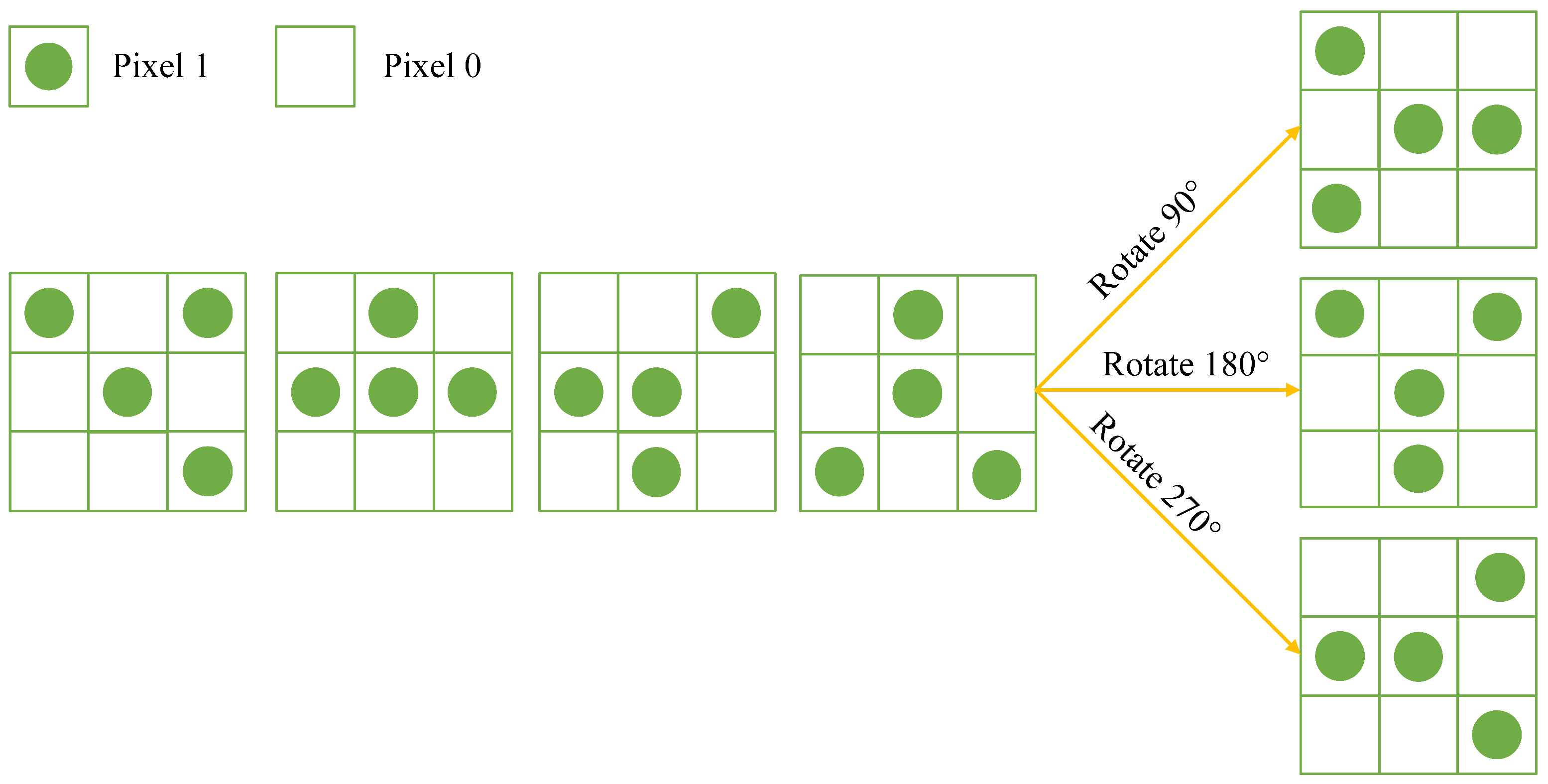
For a binary image with a line feature width of 1 pixel within the image, the branch point is defined as shown in Figure 7, using a 3 ∗ 3 window to find the branch points that match the conditions. A total of four possible structures are shown in the diagram, and it is worth noting that the structures shown in the diagram need to be rotated by 90 , 180 , and 270 during implementation of the algorithm; because the mountains in the interference fringe image have many orientations, rotations are required for each structure, i.e., there is a total of 16 possible scenarios.
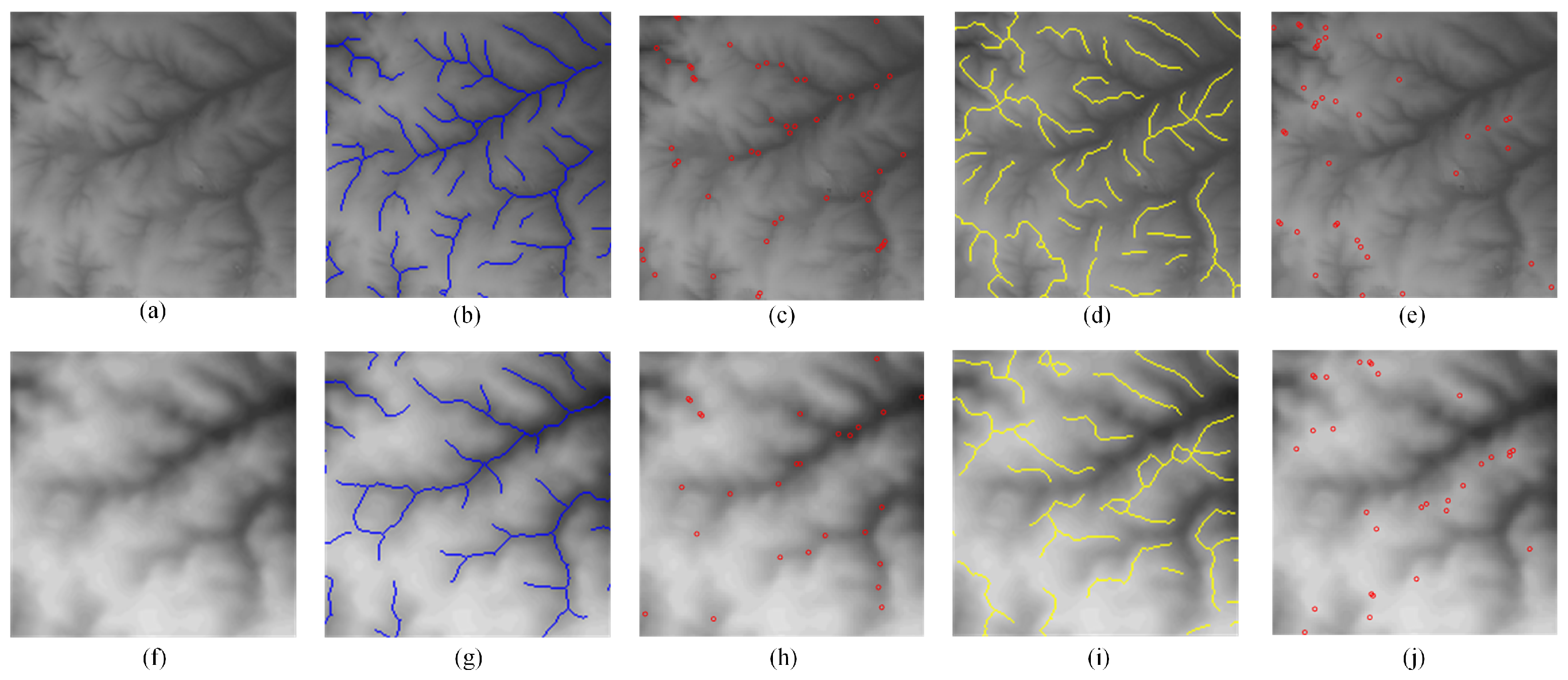
Branch points can be detected by traversing each point on the mountain range line using a 3 ∗ 3 window and determining whether its structure matches one of the 16 cases above. The detection results are shown in Figure 8, where Figure 8a,f show the real and reference interference fringes, respectively, and Figure 8c,e show the branch points detected by the ridge line diagram in Figure 8b and the valley line diagram in Figure 8d, respectively, as well as the branch points detected by the reference interference fringes in the second column. It can be seen that the range lines detected by the real interference fringes with higher resolution are more correct, the range lines detected by the reference interference fringes can reflect the overall terrain direction, and the branch points detected by both are evenly distributed and basically correspond to each other.
The analysis above only includes interference terrain that is hidden within the same range of [ π , π ] . In reality, due to inaccurate baseline parameter estimation, the interference fringe may still exhibit phase winding after removing the leveling effect, and phase mutation may occur near the phase winding area [39]. Consequently, when detecting the mountain line using the above method, the change in the eigenvalue caused by the phase mutation will also be detected, which may lead to the detection of some keypoints that are not the branch points of the mountain. Figure 9a illustrates an interference fringe with phase winding, where the winding phase is visible in the upper left corner of the image. Figure 9b shows the result of calculating the eigenvalue of the Hessian matrix for this interference fringe. It can be observed that the absolute value of the calculated eigenvalues near the phase mutation is very large. Two lines of data were selected from the eigenvalue graph of Figure 9b for slice display. The slice shown by the red dotted line passes through the phase mutation region, and the absolute value of the slice result is shown in Figure 9c. The section shown by the green dotted line does not contain the phase mutation region, and the section results are shown in Figure 9d. Upon observing Figure 9c, it can be seen that the phase mutation causes a significant change in the eigenvalues, which is much greater than the change caused by the fluctuation of the mountain range. Therefore, a phase mutation threshold with a threshold size of 3 is considered, as shown by the blue dotted line in Figure 9c, and the magnitude of the eigenvalues of the point is judged by the branch points of the mountain range detected by the above method. If the threshold exceeds this value, it can be concluded that it is caused by the phase mutation, and therefore, it does not belong to the branch point of the mountain range. Figure 9d shows the eigenvalue slice that does not pass through the phase mutation region. The correct ridge line and valley line can be detected by setting the T r i d g e and T v a l l e y values as described above.
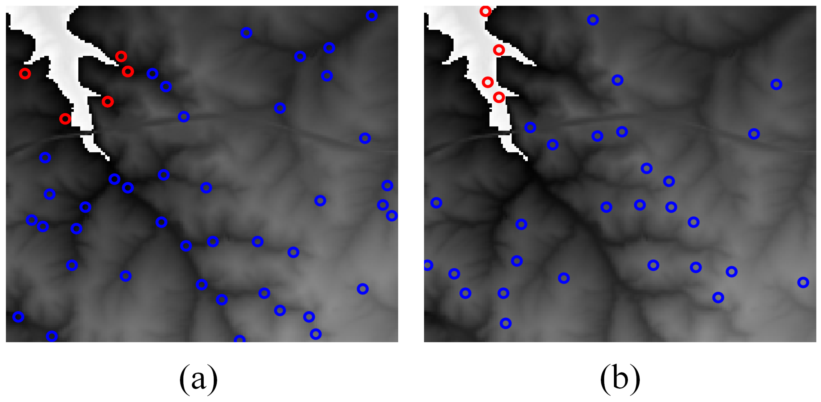
In the demonstration area of interference fringes with phase mutation shown in Figure 9a, mountain branch points were detected separately. The red circles represent false detection points that are about to be eliminated, while the blue circles represent correct mountain branch points. Figure 10a shows the detection result of the valley line branch points, and Figure 10b shows the detection result of the ridge line branch points. It can be observed from the red circles in the figure that they are all located near the phase mutation region. It can be proven that by setting a threshold, false detection points caused by phase mutation can be eliminated completely. In addition, the correctly detected mountain branch points are distributed relatively evenly, which satisfies the requirements of subsequent feature matching.

2.5. Description of Mountain Branch Points

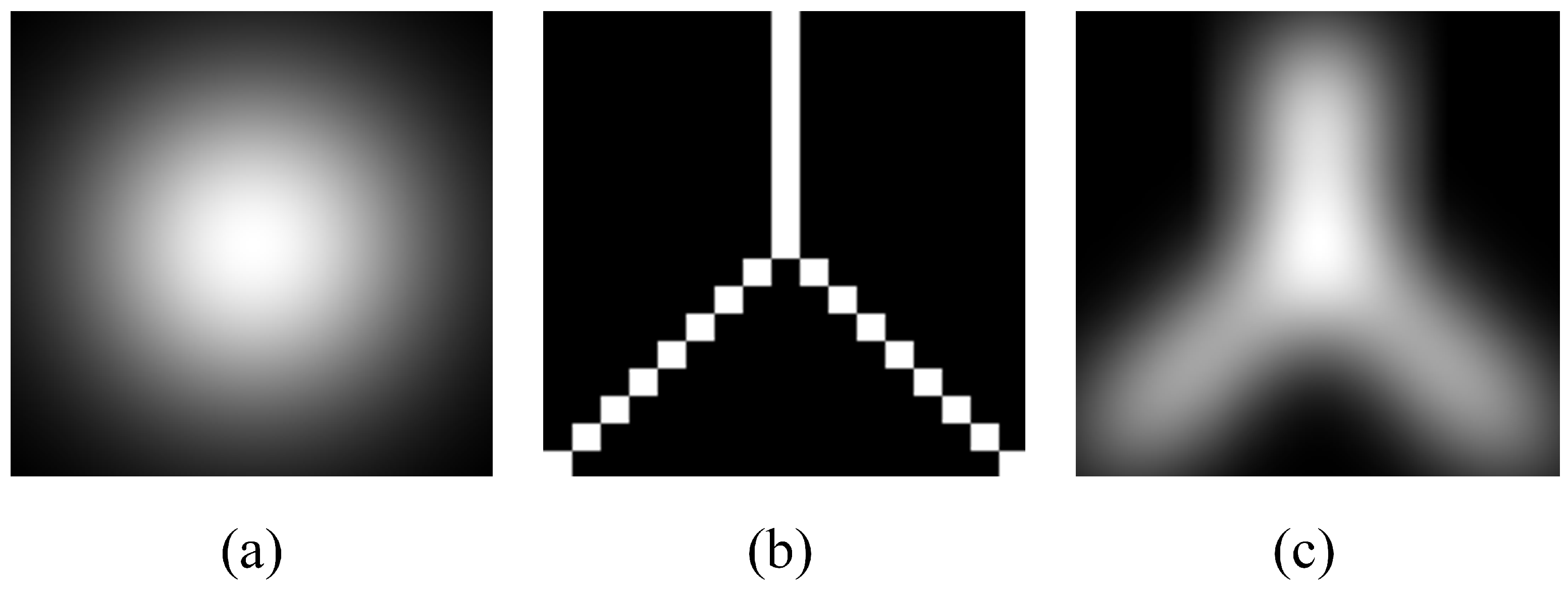
In order to successfully complete the subsequent matching task, it is also necessary to characterize each branch point. In the design of the feature description sub-stage, we have considered an enhancement to the SIFT algorithm for this study. The SIFT algorithm is designed with the idea of vectorizing the overall features of the pixels around the keypoint. The area around the keypoints is divided into 4 ∗ 4 windows, and the histograms of gradients in 8 directions within each window are calculated to generate feature descriptors. Before it is calculated, the gradient needs to be filtered using a Gaussian function, as shown in Figure 11a. This is equivalent to a distance weight, wherein a pixel that is found closer to the feature point is considered more important. This Gaussian function is improved upon in this study to solve the problem that the textures of different mountains are too similar. Figure 11b shows the range line features around the branch points extracted above. The extracted mountain range line features around the branch points are first convolved with a Gaussian function to obtain a filter, as shown in Figure 11c, which is then involved in the subsequent filtering operation. This allows the features of the mountains around the branch points to be incorporated into the feature descriptors, making them more specific to each other. This operation reflects the uniqueness of each branch point and increases the success rate of the match.
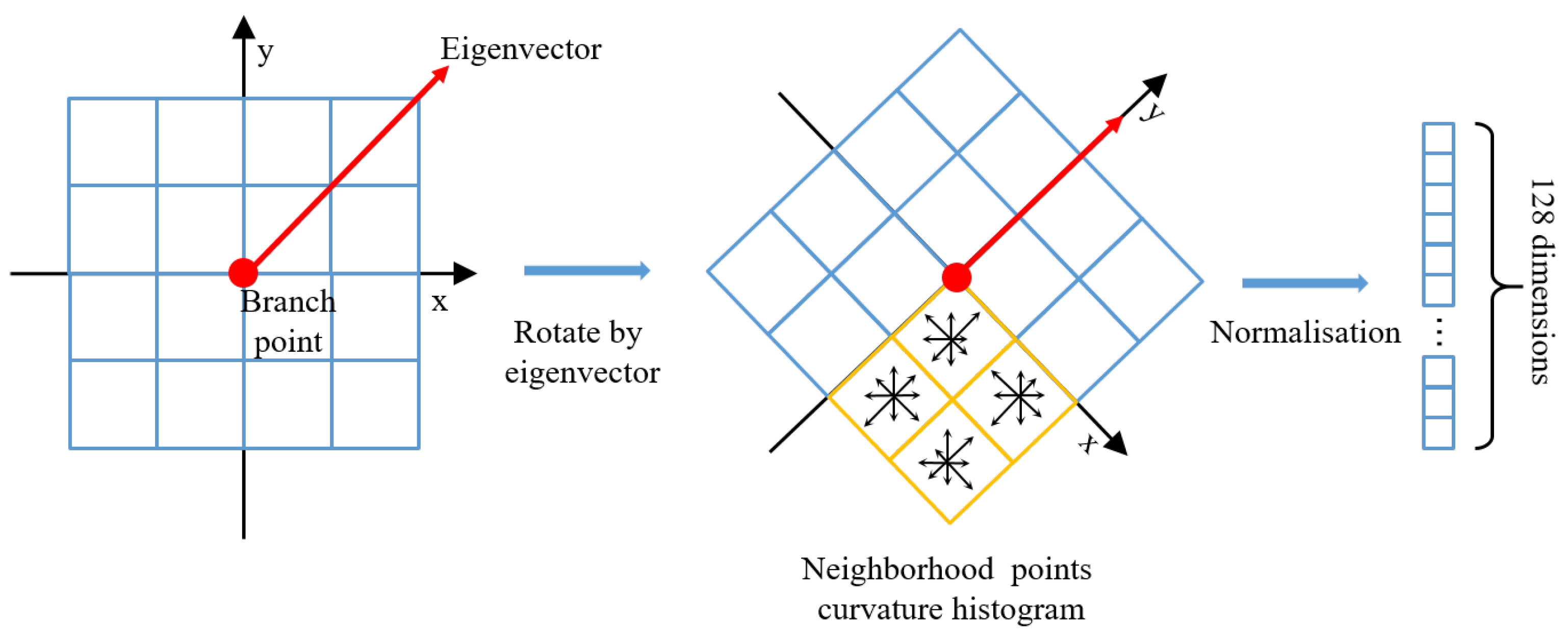
According to the discussion in Section 2.3, the idea of finding the gradient only applies to corner points in the image, whereas the branching points for interference fringe extraction originate from ridge lines or valley lines, which are not corner points, and it is therefore not appropriate to directly follow the steps of the SIFT algorithm. However, the overall idea of using the SIFT algorithm on surrounding pixels to describe keypoints is feasible. Considering that the eigenvalues and eigenvectors of the Hessian matrix have been calculated for the detection of mountain line features, the eigenvalues of the branch points represent the magnitude of the curvature at that location, and the eigenvectors represent the direction of the curvature. Therefore, the improvements shown in Figure 12 were considered. The direction of the branch point feature vector is known, and to make the descriptor rotationally invariant to accommodate errors in aircraft attitude, the pixels around the branch point need to be rotated to that direction. All pixel points around a branch have eigenvalues and eigenvectors, which also represent the magnitude and direction of curvature. The curvature of all the pixel points within the 4 ∗ 4 grid of its surrounding area is calculated, and the radius of the area is calculated according to Equation (9), where δ represents the Gaussian scale used to extract the mountain range lines in Section 2.3, and d represents the number of divisions into a grid, which is 4 in this paper. Each grid is divided into eight directions, and the magnitude of the curvature contained in each direction is determined such that a 128-dimensional branch point descriptor is constructed. After all branch point descriptors have been extracted, a normalization operation is performed to increase the efficiency of matching.
r a d i u s = 3 2 δ ( d + 1 ) + 1 2
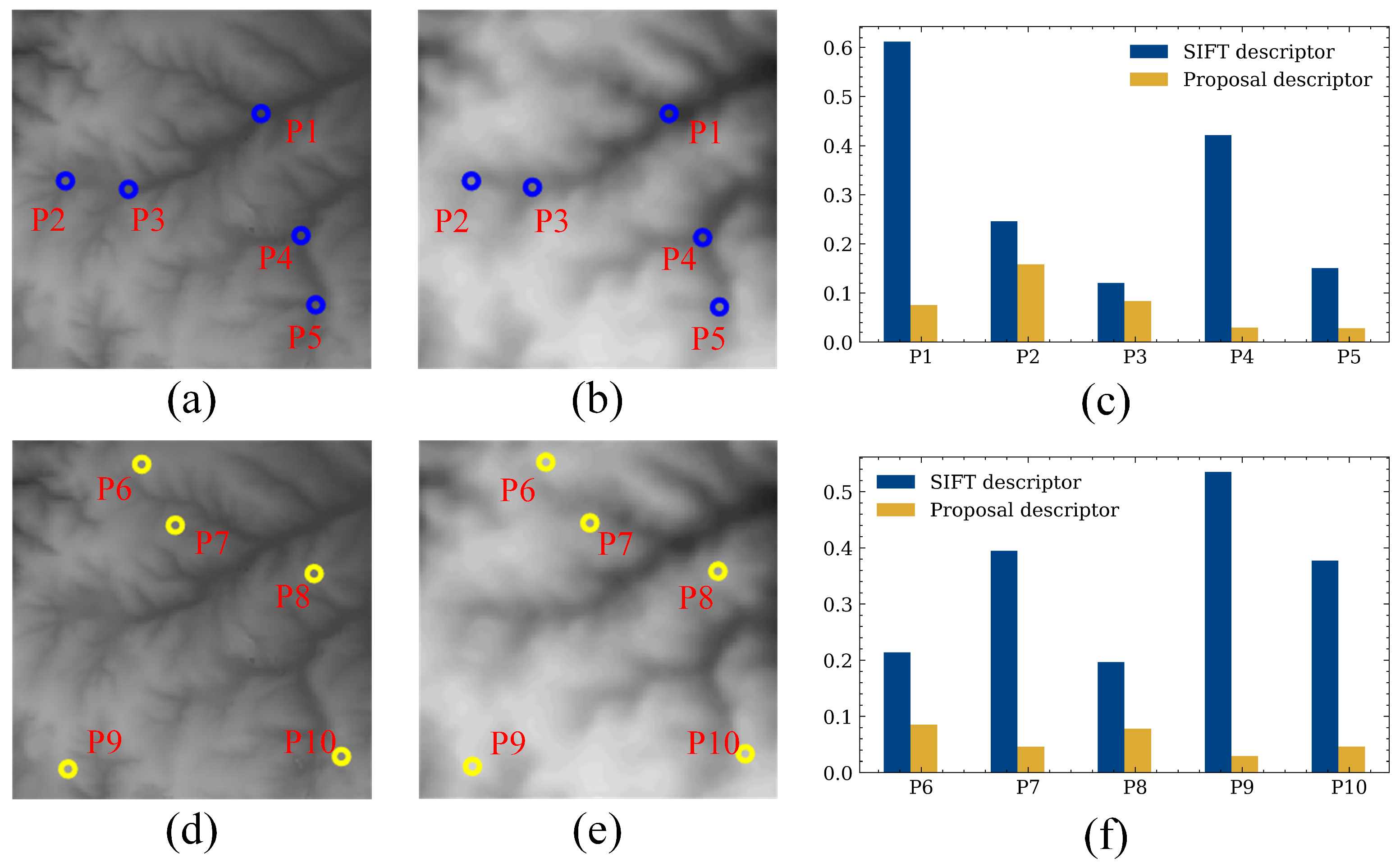
This improved descriptor has two advantages. Based on the analysis above, SIFT extracts descriptors on a gradient basis, which is applicable to corner points but not to points on ridge lines and valley lines and should be replaced with the eigenvalue as well as the orientation of the Hessian matrix when describing the surrounding pixels. The eigenvalue and eigenvector maps of the interference fringes have already been calculated in Section 2.3 and do not need to be calculated again in this section, thus saving computing time. To quantitatively compare the advantages of the improved descriptors, the following experiments were carried out. Figure 13 shows the branch points detected in the real interference fringes as well as in the reference interference fringes. Ten pairs of homonymous points that can be correctly corresponded are selected, which are divided into five pairs of valley branch homonymous points P1–P5, as shown in Figure 13a,b, and five pairs of ridge branch homonymous points, as shown in Figure 13d,e. The SIFT descriptors for these ten pairs of points and the distances of the improved descriptors at Euclidean distances are calculated, and the statistics are shown in Figure 13c,f. It can be seen that the improved descriptors are significant improvements over SIFT at Euclidean distances for both ridge line branch points and valley line branch points.

3. Results

3.1. Experimental Data

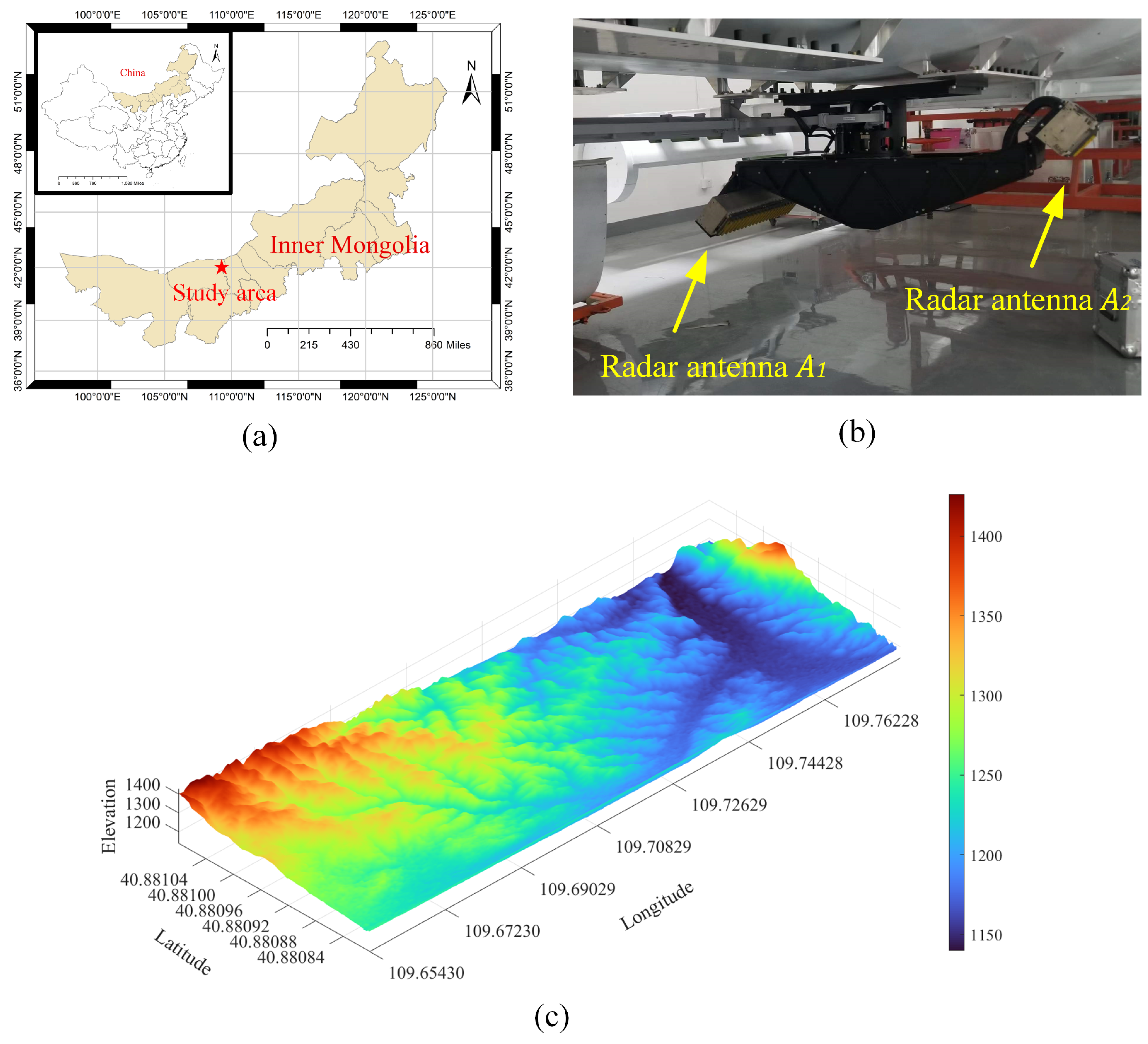
For experimental verification in this study, we utilized interference fringes that were acquired during actual flight tests. These flight tests were conducted in Baotou, Inner Mongolia, China. Figure 14a shows the specific location of the experimental site. The aircraft model is Modern Ark 60. The radar model is X-band dual-antenna radar with a bandwidth of 300 MHz. The radar is shown in Figure 14b. The radar is located at the bottom of the aircraft. Figure 14c shows the DEM data of the experimental scene. It can be seen that the terrain of the experimental site fluctuates greatly, which can verify the extraction effect of the proposed algorithm for terrain features. Flight-related parameters are shown in Table 2, where R m i n is the nearest slant distance, S a is the azimuthal resolution, S r is the range resolution, and the remaining parameters are described in Section 2.2.
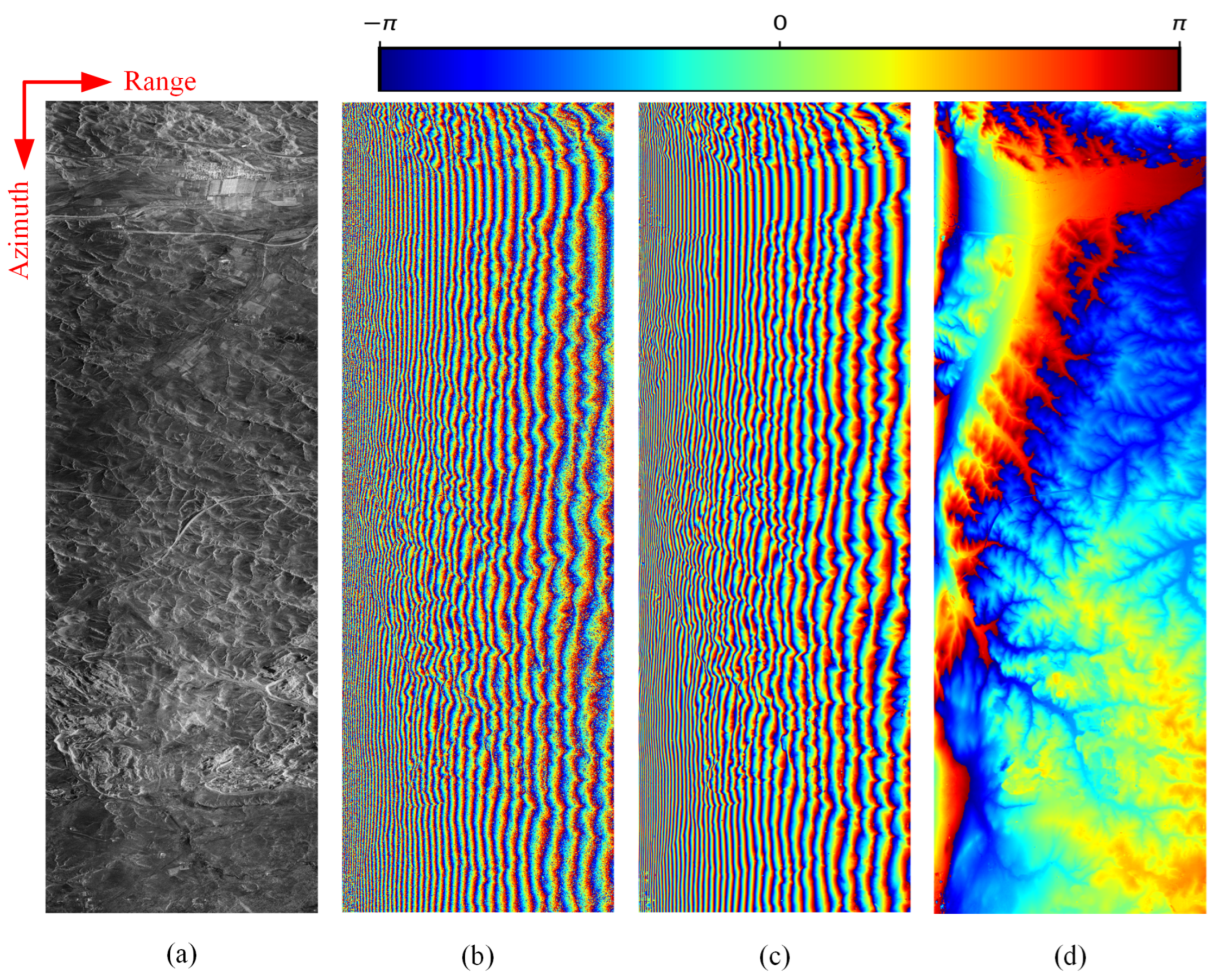
Figure 15a shows an SAR image obtained in the experiment. The number of azimuth points is 16,384, and the number of range points is 5500. A pair of SAR echo data points obtained in the experiment are registered to obtain the interference phase, as shown in Figure 15b. Classic interference phase denoising technology [40] is used to remove the noise. The interference fringe image after noise removal is shown in Figure 15c. To make the terrain feature more obvious, the phases of flat earth of the interference fringe need to be removed [41], as shown in Figure 15d. It can be seen that the interference fringes caused by the phase of the flat ground were removed, but there are still some fringes in the image, which is caused by the excessive undulation of the terrain. Due to the low resolution of the reference interference fringes, the actual interference fringes were down-sampled to ensure that they have the same proportion as the actual interference fringes.
The reference interference fringes were generated using DEM data that were derived from the publicly available NASA/ALOS PALSAR dataset. The resolution of the DEM data used was 12.5 m. Assuming that there are no errors in the POS data during the actual flight of the aircraft, the reference interference fringes for the corresponding region are generated according to the method in [42], as shown in Figure 16a. Compared with Figure 14f, it can be seen that the phase winding of the reference interference fringe is different from the real data. This is because the positioning and orientation system (POS) data of the actual flight are not ideal. This situation is in line with the actual situation and also tests the effectiveness of the algorithm. To verify the effectiveness of the algorithm in correcting the errors accumulated by the inertial measurement unit (IMU) during the flight of a real aircraft, two reference interference fringe datasets are produced, corresponding to a position error experiment and an attitude error experiment. The first dataset is generated by artificially adding position errors in the process of simulating interference fringes. The real position errors that exist in flight are simulated. The azimuth errors range between plus and minus 500 m, with an error interval of 25 m. A total of 41 datasets is generated. Figure 16b shows an example of interference fringes with position errors, in which the azimuth error is −500 m and the distance error is −500 m. It can be seen that the interference fringes with position errors are shifted in both azimuth and distance directions compared with the interference fringes without errors. The second dataset is generated by artificially adding yaw angle error in the process of simulating interference fringes to simulate the real attitude error in flight, where the yaw angle error is between plus and minus 30 , the error interval is 1 , and there is a total of 61 pieces. Figure 16c shows an example of interference fringes with attitude error, where the yaw angle error is 30 . It can be seen that the interference fringes with attitude errors have certain rotation and translation compared with the interference fringes without errors.

3.2. Position Error Experiment and Attitude Error Experiment

To verify the effectiveness of the proposed method, the proposed algorithm is compared with other image matching algorithms under the above two error conditions, and a position error experiment and attitude error experiment are carried out. Since no matching algorithms have been reported for interference fringe data, comparisons with the classic algorithms SIFT and SURF are presented in this paper.
The parameters for the proposed algorithm are set as follows: the scale of the Gaussian function is set to 2, T r i d g e is set to 0.7 and T v a l l e y is set to −0.7. The threshold value for eliminating the mountain branch points that are detected by mistake due to the interference phase mutation is set to 3, the grid size around the branch point is selected as 4*4 in the generation description sub-stage, and the radius around the branch point is calculated according to Equation (9). Point pairs less than 0.6 under the Euclidean distance are identified as homonymous points, the RANSAC algorithm is set with an error threshold less than 1, and the number of iterations is 2000.
To objectively compare the strengths and weaknesses of different algorithms, the evaluation metrics used in this paper are inliers, precision, recall, and the overall evaluation metric (F1-Score). Precision is defined as the number of inliers filtered by RANSAC divided by the number of correspondences output by the algorithm, and it evaluates the effect of the designed descriptor. Recall is defined as the number of correspondences actually correct among all the feature pairs calculated by the algorithm. Recall evaluates the value of the algorithm in finding keypoints. F1-Score evaluates the overall performance of the algorithm, and the three are defined as follows:
P r e c i s i o n = I n l i e r s M a t c h e s R e c a l l = I n l i e r s C o r r e s p o n d e n c e P r e c i s i o n = 2 P r e c i s i o n R e c a l l P r e c i s i o n + R e c a l l
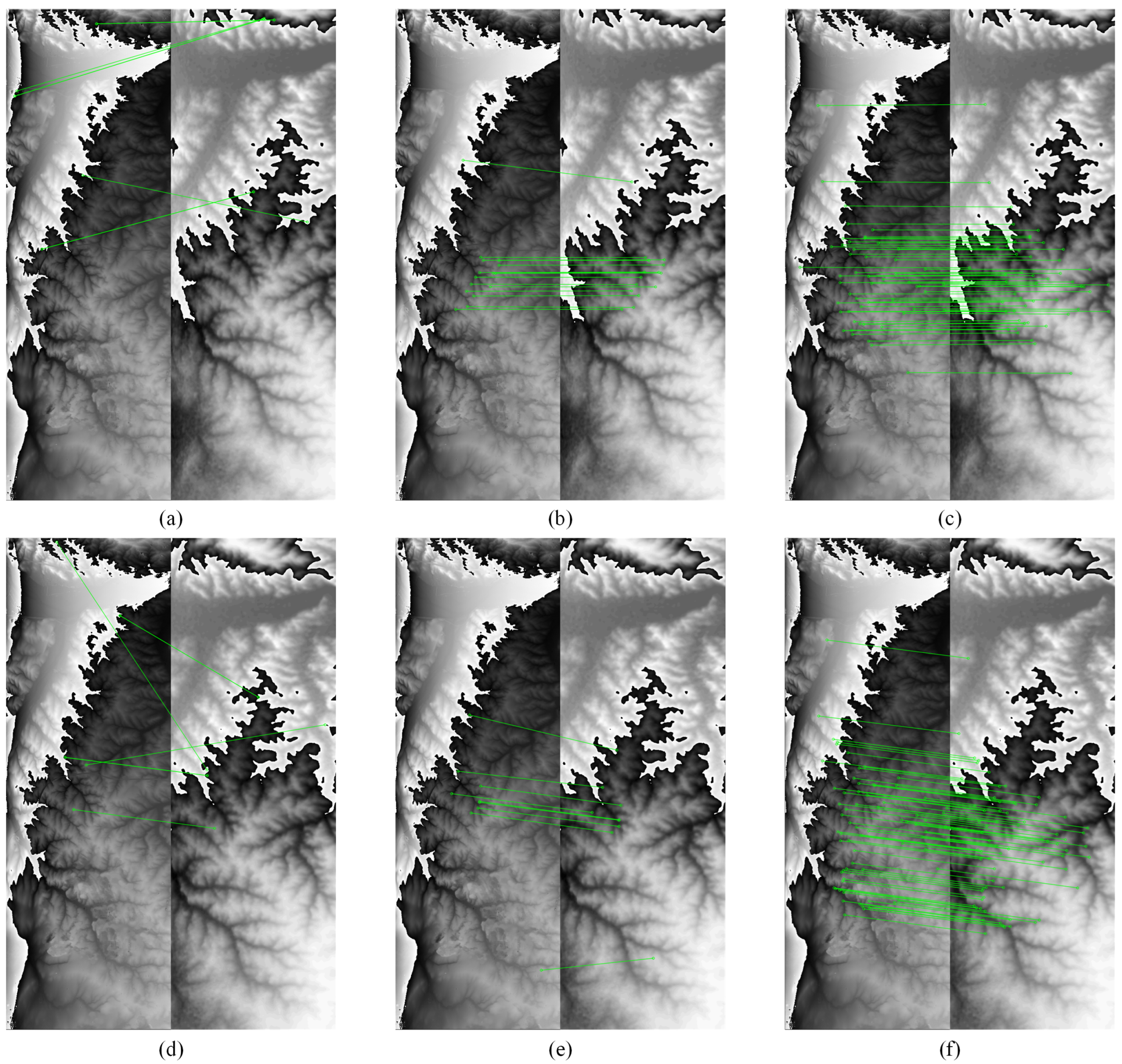
First, the position error experiment is shown. Figure 17a–c show the matching results of the three algorithms without any error, and the matching results were eliminated by the RANSCA algorithm. From Figure 17a, we can see that the SIFT algorithm does not obtain the correct matching point, which means that it is completely mismatched; Figure 17b shows the matching results of the SURF algorithm. The algorithm obtains fewer correct matching points and there are wrong matching items; Figure 17c shows the matching results of the proposed algorithm, which obtains the most correct matching points. Figure 17d–f shows the matching results of the 3 algorithms under the conditions of simulated interference fringe azimuthal error −500 m and range error −500 m. It can be seen from Figure 17d and Figure 17e that the matching results of the algorithms participating in the comparison are still poor under error conditions, while from Figure 17f it can be seen that the algorithm can still achieve stable and correct results under error conditions.
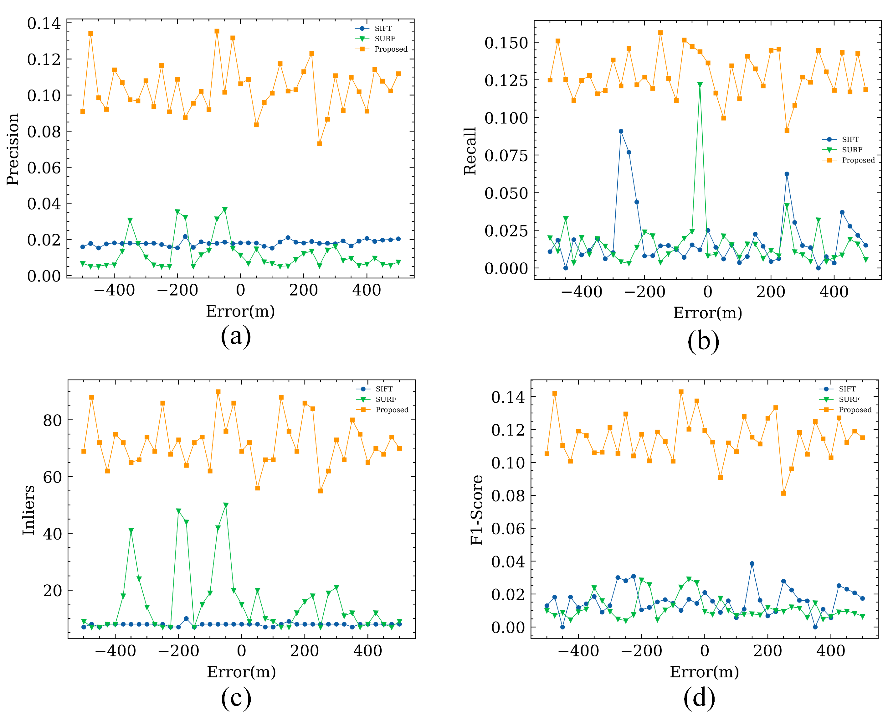
To quantitatively describe algorithm performance, the above algorithm is run under the dataset of 41 simulated interference fringes with a positional error of plus or minus 500 m and an error interval of 25 m. Inliers, precision, recall, and F1-Score are quantified, and the results are shown in Figure 18. The mean values of the quantitative evaluation metrics are shown in Table 3.
As seen in the quantitative comparison results above, the SIFT algorithm extracted an average of only about 8 inliers, demonstrating that the algorithm is not sufficiently robust when applied to the interference fringe position error dataset. Although the SURF algorithm extracted more inliers, the values for its three indicators of recall and F1-Score were the worst of the three algorithms, indicating that, although the SURF algorithm extracted more points, its matching success rate is poor and its overall performance was not good. In comparison, the average number of inliers extracted by the proposed algorithm reached about 72, indicating that the algorithm is highly robust and can adapt to the needs of aircraft IMU for matching algorithms in a position error environment. The average precision of this algorithm is 0.103, which is higher than that of the two other algorithms, indicating that the branch points extracted by the algorithm are more valuable than those extracted using the two other algorithms. The average recall of this algorithm is 0.128, which is higher than that of the remaining two algorithms. As seen in Figure 18b, although the recall of SIFT and SURF is good in several groups of experiments, it again proves the poor stability of SIFT and SURF due to large up-and-down fluctuations. As seen in Figure 18d as well as Table 3, the comprehensive performance of this algorithm is better than that of the two other algorithms.
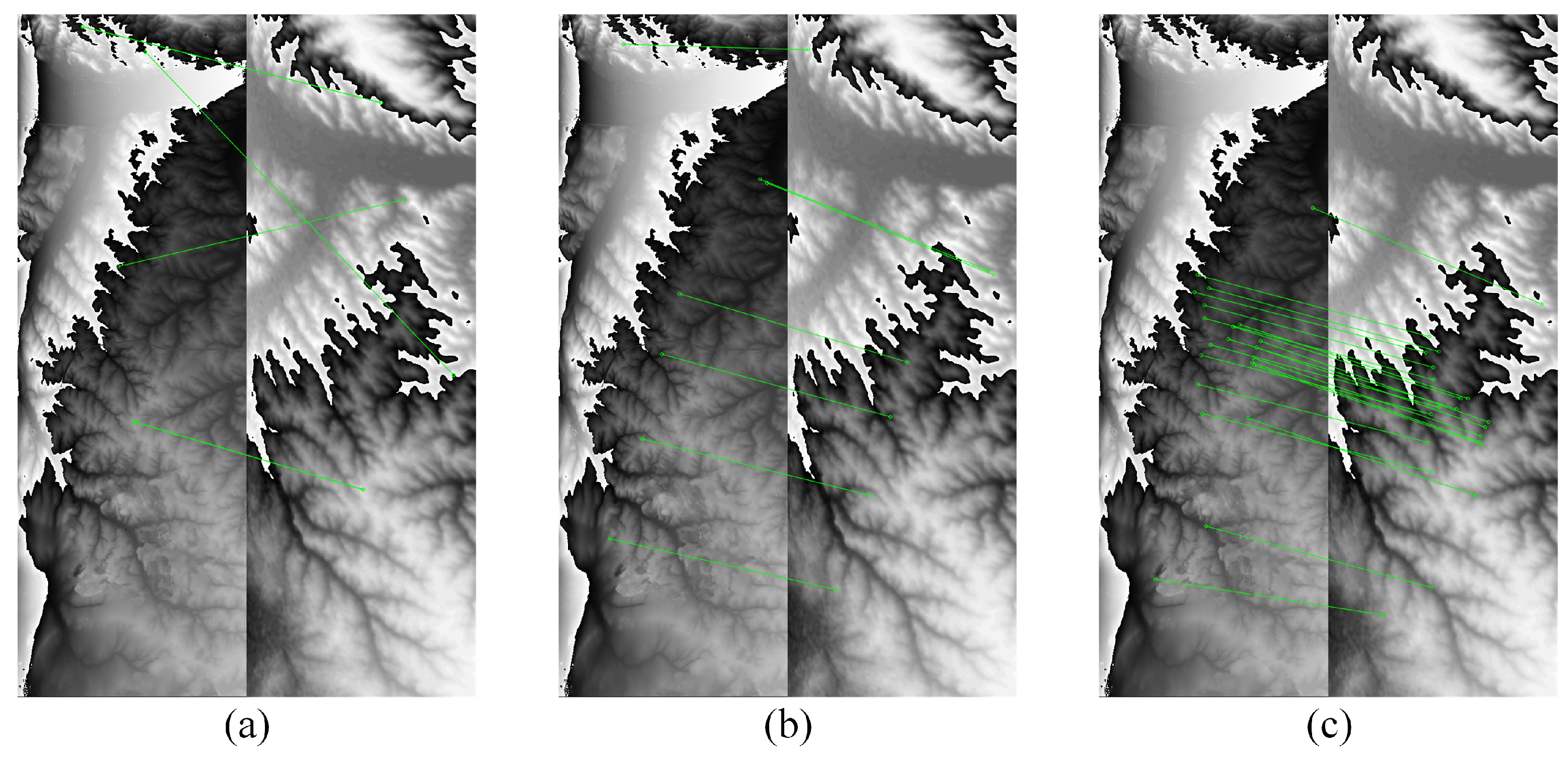
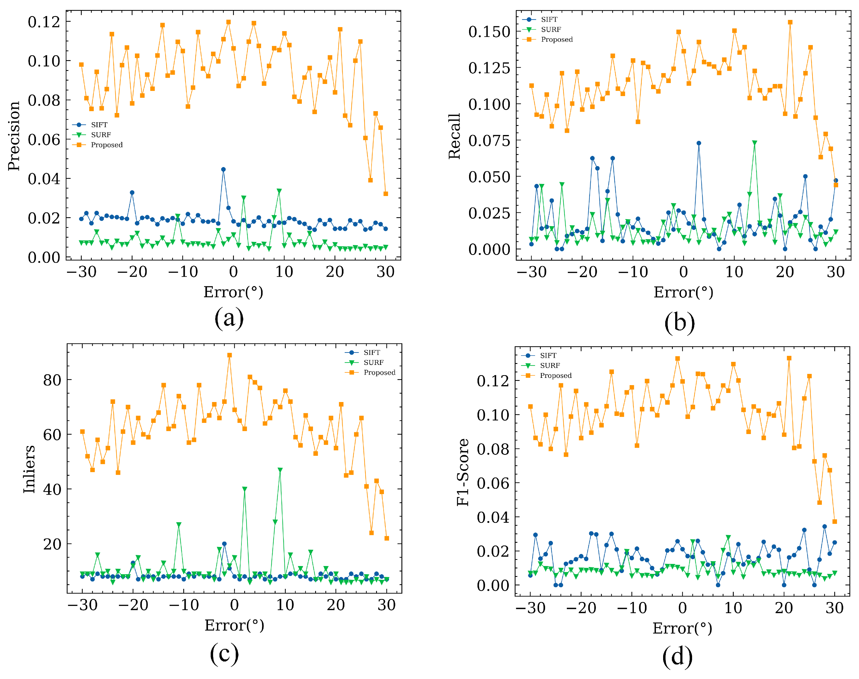
Second is the attitude error experiment. Figure 19 shows the matching effect of the three algorithms when the simulated interference fringes have a thirty degree yaw angle error. Figure 19a–c show the SIFT algorithm, SURF algorithm, and the algorithm proposed in this paper, respectively, and outlier points were eliminated in all three algorithms. The number of correct matching points obtained by the proposed algorithm is still the largest when the interference fringes are rotated and shifted.
To quantitatively describe the algorithm performance, the above algorithm is run on the dataset of 61 simulated interference fringes with a yaw angle error of plus or minus 30 and an error interval of 1 . Inliers, precision, recall, and F1-Score were quantified, and the results are shown in Figure 20. The mean values of the quantitative evaluation metrics are shown in Table 4.
From the above quantitative comparison results, it can be seen that the average number of inliers extracted by the SIFT algorithm is 8, which demonstrates that the SIFT algorithm is still not robust when applied to the attitude error dataset. Although the SURF algorithm extracts many inliers, its precision, recall and F1-Score are the worst among the three algorithms. In contrast, the average number of inliers extracted by this algorithm is about 62, the average precision is 0.093, the average recall is 0.112, and the F1-Score is 0.108, which is higher than the other two algorithms. This proves that the algorithm is effective and can meet the requirements of the aircraft IMU for the matching algorithm in the attitude error environment.
It can be seen in Figure 20 that, when the attitude error is large, the effects of the three algorithms are reduced, which is in line with the actual situation. In general, the proposed algorithm is still optimal.

4. Discussion

Based on the information presented in Table 3 and Table 4, it is clear that the traditional algorithm fails to achieve accurate matching, while the proposed algorithm has shown promising results. Our analysis suggests that there may be two reasons for this discrepancy. First, the traditional algorithm mainly describes the feature points through a gradient, which has no physical significance in the interference fringes. However, the proposed algorithm excavates the rich terrain features contained in the interference fringes to serve the matching task, so it can achieve good results. Second, the interference phase will inevitably feature phase winding, and phase winding will bring with it phase mutation. Although it is mentioned in Section 3.1 that we assume that there is no error in the POS data of the aircraft, there will still be some error in the actual flight process, which will lead to the difference between the winding of the reference interference fringe retrieved from the DEM data and the actual interference fringe; this can be seen from Figure 15d and Figure 16a. The traditional algorithm will detect a large number of key points in the phase mutation region, because the winding situation of the reference interference fringes is different from that of the measured interference fringes, which will cause the two to be unable to be matched correctly. Through the analysis results in Figure 9, this algorithm designs a threshold to eliminate the false detection caused by phase mutation, thus avoiding this situation. Figure 17 and Figure 19 illustrate the matching results, revealing that the traditional algorithm is prone to detecting incorrect matching points in the phase mutation region. In contrast, the proposed algorithm does not encounter this issue and can identify matching points across different winding cycles.
Figure 18 shows that the indicators of the proposed algorithm are stable under different error values, and matching does not decrease when the error value becomes larger. Table 4 shows the average results of the attitude error experiments. The quantitative index of the proposed algorithm is still superior to that of the traditional algorithm, demonstrating that the proposed algorithm can meet different error requirements, which is critical in the actual flight process. It can be seen in Figure 20 that the matching effect of the three algorithms, including the proposed algorithm, decreases due to the larger error value. This is because the interference fringes with yaw angle error not only have rotation displacement but also a certain degree of expansion transformation, which has a great impact on the matching effect. Therefore, improvements on this point can be addressed in subsequent research.
Let us discuss the accuracy of the proposed algorithm. Accurate matching of interference fringes requires ensuring that the actual branching points of the real interference fringes are the same as those of the reference interference fringes. This paper first obtains line features with a pixel width of 1 by performing threshold segmentation and skeletonization on the eigenvalue map of the interference fringes. Then, it detects the branch points of the mountain using a branch point template. This image processing operation cannot guarantee that the detected branch points in the real data and reference data correspond exactly in position, introducing errors, which can be defined as E i . This algorithm introduces mountain line thresholds and phase mutation thresholds, which are hard thresholds that cannot fully and accurately detect mountain line features, and can also introduce errors, which are defined as E t . The DEM data resolution required to generate the reference interference fringes cannot be guaranteed to be consistent with the real interference fringes, which can also introduce errors, defined as E s , the error introduced by different interference fringe scales. E i + E t + E s is the source of all errors in this algorithm, and it is the theoretical basis for optimizing the algorithm in the future.
In this study, the traditional image matching idea of directly detecting feature points is discarded, and we innovatively propose using mountain range branch points as feature points for interference fringe matching, making full use of terrain features for the matching task. It can be seen from the experiments that the proposed algorithm has good results for matching interference fringe data, which opens up new ideas for subsequent research. This line of thought also applies to other data with topographical information, such as DEMs. It is worth noting that, since the reference interference fringe data are interpolated from the scale of the measured data, the algorithm does not take into account the effect of scale on the algorithm, but this needs to be taken into account if it is used for other tasks. The algorithm mentioned in the paper is based on the operation of the image domain and uses a more traditional principle. The extracted branch points are not accurate to the subpixel level, and the downstream matching task would benefit from more accurate means of detecting mountain line features.

5. Conclusions

The main objective of this study was to address the primary technical challenge associated with using interference fringe matching for navigation, namely, the poor performance of traditional algorithms in this context. First, the image characteristics of interference fringes were analyzed, and it is concluded that traditional algorithms fail to make use of the rich terrain features of interference fringes, which leads to a poor matching effect. Based on this, the proposed algorithm was first designed to extract the mountain line features and to detect the branch points of the mountain range as the keypoints for feature matching based on the online features; second, the SIFT descriptor was improved by using the terrain features around the branch points. Using real measurement data, we demonstrated that the results are significantly improved compared with those of the traditional algorithm, providing a new idea for terrain data matching. The method proposed in this paper can accurately detect mountain lines using the algorithm. Future research should focus on improving the accuracy of mountain line detection, which will enhance the algorithm’s performance. As the algorithm detects the mountain branch point at a non-sub-pixel level, it is also worth exploring methods to locate the mountain branch point at sub-pixel level. Additionally, an interference fringe is an image with topographic features, and the method proposed in this paper is based on this feature. Therefore, the study of any remote sensing image matching problem with terrain features can be inspired by this paper.

Author Contributions

Conceptualization, B.W., M.X., N.L. and G.S.; investigation, G.S. and L.L.; software, G.S. and R.S.; writing—original draft preparation, G.S.; writing—review and editing, G.S., L.L. and Y.W. All authors have read and agreed to the published version of the manuscript.

Funding

This work was supported by the National Natural Science Foundation of China under Grant No. 62073306. This work was also supported by the Youth Innovation Promotion Association CAS.

Institutional Review Board Statement

Not applicable.

Informed Consent Statement

Not applicable.

Data Availability Statement

The DEM data demonstrated by Figure 14b and the DEM data needed to generate the reference interference fringe can be downloaded from the link: https://search.asf.alaska.edu/, accessed on 1 March 2022.

Acknowledgments

The authors thank the staff of the National Key Laboratory of Microwave Imaging Technology, Aerospace Information Research Institute, Chinese Academy of Sciences, for their valuable conversations and comments.

Conflicts of Interest

The authors declare no conflict of interest.

References

  1. Savage, P.G. Strapdown inertial navigation integration algorithm design part 2: Velocity and position algorithms. J. Guid. Control Dyn. 1998, 21, 208–221. [Google Scholar] [CrossRef]
  2. Zhou, Y.; Wan, J.; Li, Z.; Song, Z. GPS/INS integrated navigation with BP neural network and Kalman filter. In Proceedings of the 2017 IEEE International Conference on Robotics and Biomimetics (ROBIO), Macau, China, 5–8 December 2017; pp. 2515–2520. [Google Scholar] [CrossRef]
  3. Sun, B.; Yan, W.-D.; Ma, X.-L.; Bian, H.; Ni, W.-P.; Zheng, G. A new scene matching algorithm during optical aided navigation of aircraft. In Proceedings of the 2012 International Conference on Image Analysis and Signal Processing, Agadir, Morocco, 28–30 June 2012; pp. 1–4. [Google Scholar] [CrossRef]
  4. Greco, M.; Pinelli, G.; Kulpa, K.; Samczynski, P.; Querry, B.; Querry, S. The study on SAR images exploitation for air platform navigation purposes. In Proceedings of the 2011 12th International Radar Symposium (IRS), Leipzig, Germany, 7–9 September 2011; pp. 347–352. [Google Scholar]
  5. Kedong, W.; Yang, Y. Influence of application conditions on terrain-aided navigation. In Proceedings of the 2010 8th World Congress on Intelligent Control and Automation, Jinan, China, 7–9 July 2010; pp. 391–396. [Google Scholar] [CrossRef]
  6. Buck, T.; Wilmot, J.; Cook, M. A High G, MEMS Based, Deeply Integrated, INS/GPS, Guidance, Navigation and Control Flight Management Unit. In Proceedings of the IEEE/ION PLANS 2006, San Diego, CA, USA, 25–27 April 2006; pp. 772–794. [Google Scholar]
  7. Massonnet, D.; Feigl, K.L. Radar interferometry and its application to changes in the Earth’s surface. Rev. Geophys. 1998, 36, 441–500. [Google Scholar] [CrossRef] [Green Version]
  8. Greco, M.; Kulpa, K.; Pinelli, G.; Samczynski, P. SAR and InSAR georeferencing algorithms for inertial navigation systems. In Proceedings of the Photonics Applications in Astronomy, Communications, Industry, and High-Energy Physics Experiments, Wilga, Poland, 3–10 June 2011; p. 80081O. [Google Scholar] [CrossRef]
  9. Nitti, D.O.; Bovenga, F.; Morea, A.; Rana, F.; Guerriero, L.; Greco, M.; Pinelli, G. On the use of SAR interferometry to aid navigation of UAV. In Remote Sensing of the Ocean, Sea Ice, Coastal Waters, and Large Water Regions; SPIE: Bellingham, WA, USA, 2012; Volume 8532. [Google Scholar] [CrossRef]
  10. Shuai, J.; Maosheng, X.; Bingnan, W.; Xikai, F.; Yinwei, L.; Weiran, S.; Yu, Y. The method of InSAR/INS integrated navigation. In Proceedings of the 2016 CIE International Conference on Radar (RADAR), Guangzhou, China, 10–13 October 2016; pp. 1–4. [Google Scholar] [CrossRef]
  11. Sun, G.; Dong, J.; Yang, A.; Wu, J. Extraction of Interference Fringe Information Based on Self-adaptive Restoration and Clustering via Distance Histogram. In Proceedings of the 2006 6th World Congress on Intelligent Control and Automation, Dalian, China, 21–23 June 2006; Volume 2, pp. 10342–10346. [Google Scholar] [CrossRef]
  12. Jiang, S.; Wang, B.N.; Xiang, M.S.; Fu, X.K.; Li, Y.W. An Inversion Method of the Attitude for InSAR/INS Integrated Navigation. Tien Tzu Hsueh Pao/Acta Electron. Sin. 2018, 46, 513–519. [Google Scholar]
  13. Lowe, D. Distinctive image features from scaleinvariant keypoints. Int. J. Comput. Vis. 2004, 60, 91–110. [Google Scholar] [CrossRef]
  14. Bay, H.; Ess, A.; Tuytelaars, T.; Van Gool, L. Speeded-Up Robust Features (SURF). Comput. Vis. Image Underst. 2008, 110, 346–359. [Google Scholar] [CrossRef]
  15. Rublee, E.; Rabaud, V.; Konolige, K.; Bradski, G. ORB: An efficient alternative to SIFT or SURF. In Proceedings of the 2011 International Conference on Computer Vision, Barcelona, Spain, 6–13 November 2011; pp. 2564–2571. [Google Scholar]
  16. Rosten, E.; Drummond, T. Machine learning for high-speed corner detection. In Proceedings of the Computer Vision–ECCV 2006: 9th European Conference on Computer Vision, Graz, Austria, 7–13 May 2006; pp. 430–443. [Google Scholar]
  17. Calonder, M.; Lepetit, V.; Strecha, C.; Fua, P. Brief: Binary robust independent elementary features. In Proceedings of the Computer Vision–ECCV 2010: 11th European Conference on Computer Vision, Heraklion, Crete, Greece, 5–11 September 2010; pp. 778–792. [Google Scholar]
  18. Giveki, D.; Soltanshahi, M.A.; Montazer, G.A. A new image feature descriptor for content based image retrieval using scale invariant feature transform and local derivative pattern. Optik 2017, 131, 242–254. [Google Scholar] [CrossRef]
  19. Malkov, Y.A.; Yashunin, D.A. Efficient and robust approximate nearest neighbor search using hierarchical navigable small world graphs. IEEE Trans. Pattern Anal. Mach. Intell. 2018, 42, 824–836. [Google Scholar] [CrossRef] [PubMed] [Green Version]
  20. Raveendra, K.; Vinothkanna, R. Hybrid ant colony optimization model for image retrieval using scale-invariant feature transform local descriptor. Comput. Electr. Eng. 2019, 74, 281–291. [Google Scholar]
  21. Koch, G.; Zemel, R.; Salakhutdinov, R. Siamese neural networks for one-shot image recognition. In Proceedings of the ICML Deep Learning Workshop, Lille, France, 6–11 July 2015; Volume 2. [Google Scholar]
  22. Yi, K.M.; Trulls, E.; Lepetit, V.; Fua, P. Lift: Learned invariant feature transform. In Proceedings of the Computer Vision–ECCV 2016: 14th European Conference, Amsterdam, The Netherlands, 11–14 October 2016; pp. 467–483. [Google Scholar]
  23. DeTone, D.; Malisiewicz, T.; Rabinovich, A. Superpoint: Self-supervised interest point detection and description. In Proceedings of the IEEE Conference on Computer Vision and Pattern Recognition Workshops, Salt Lake City, UT, USA, 18–22 June 2018; pp. 224–236. [Google Scholar]
  24. Sarlin, P.E.; DeTone, D.; Malisiewicz, T.; Rabinovich, A. Superglue: Learning feature matching with graph neural networks. In Proceedings of the IEEE/CVF Conference on Computer Vision and Pattern Recognition, Seattle, WA, USA, 13–19 June 2020; pp. 4938–4947. [Google Scholar]
  25. Kampes, B.; Usai, S. Doris: The delft object-oriented radar interferometric software. In Proceedings of the of the 2nd International Symposium on Operationalization of Remote Sensing, Enschede, The Netherlands, 16–20 August 1999; Volume 1620. [Google Scholar]
  26. Werner, C.; Wegmueller, U.; Strozzi, T.; Wiesmann, A. Gamma SAR and interferometric processing software. In Proceedings of the of the Ers-Envisat Symposium, Gothenburg, Sweden, 16–20 December 2000; Volume 1620, p. 1620. [Google Scholar]
  27. Fischler, M.A.; Bolles, R.C. Random Sample Consensus: A Paradigm for Model Fitting with Applications to Image Analysis and Automated Cartography. Commun. ACM 1981, 24, 381–395. [Google Scholar] [CrossRef]
  28. Stevens, D.; Cumming, I.; Gray, A. Motion compensation for airborne interferometric SAR. In Proceedings of the of IGARSS ’94—1994 IEEE International Geoscience and Remote Sensing Symposium, Pasadena, CA, USA, 8–12 August 1994; Volume 4, pp. 1967–1970. [Google Scholar] [CrossRef]
  29. Ziguan, W.; Zhang, G.; Chengshu, W.; Xing, S. Gully Morphological Characteristics and Topographic Threshold Determined by UAV in a Small Watershed on the Loess Plateau. Remote Sens. 2022, 14, 3529. [Google Scholar] [CrossRef]
  30. Jenson, S.K.; Domingue, J.O. Extracting topographic structure from digital elevation data for geographic information-system analysis. Photogramm. Eng. Remote Sens. 1988, 54, 1593–1600. [Google Scholar]
  31. Jiang, W.; Xi, D.; Deng, X.; Huang, L.; Ying, S. Extraction of Ridge Lines from Grid DEMs with the Steepest Ascent Method Based on Constrained Direction. In Proceedings of the Advances in Cartography and GIScience, Washington, DC, USA, 2–7 July 2017; Peterson, M.P., Ed.; Springer International Publishing: Cham, Switzerland, 2017; pp. 375–387. [Google Scholar]
  32. Koka, S.; Anada, K.; Nakayama, Y.; Sugita, K.; Yaku, T.; Yokoyama, R. A Comparison of Ridge Detection Methods for DEM Data. In Proceedings of the 2012 13th ACIS International Conference on Software Engineering, Artificial Intelligence, Networking and Parallel/Distributed Computing, Kyoto, Japan, 8–10 August 2012; pp. 513–517. [Google Scholar] [CrossRef]
  33. Chen, S.C.; Chiu, C.C. Texture Construction Edge Detection Algorithm. Appl. Sci. 2019, 9, 897. [Google Scholar] [CrossRef] [Green Version]
  34. Damon, J.N. Properties of Ridges and Cores for Two-Dimensional Images. J. Math. Imaging Vis. 2004, 10, 163–174. [Google Scholar]
  35. Liu, J.; White, J.M.; Summers, R.M. Automated detection of blob structures by Hessian analysis and object scale. In Proceedings of the 2010 IEEE International Conference on Image Processing, Hong Kong, China, 26–29 September 2010; pp. 841–844. [Google Scholar] [CrossRef]
  36. Kimmel, R.; Shaked, D.; Kiryati, N.; Bruckstein, A.M. Skeletonization via Distance Maps and Level Sets. Comput. Vis. Image Underst. 1995, 62, 382–391. [Google Scholar] [CrossRef]
  37. Golland, P.; Eric, W.; Grimson, L. Fixed topology skeletons. In Proceedings of the IEEE Conference on Computer Vision and Pattern Recognition. CVPR 2000 (Cat. No.PR00662), Hilton Head, SC, USA, 13–15 June 2000; Volume 1, pp. 10–17. [Google Scholar] [CrossRef]
  38. Abeysinghe, S.S.; Baker, M.; Chiu, W.; Ju, T. Segmentation-free skeletonization of grayscale volumes for shape understanding. In Proceedings of the 2008 IEEE International Conference on Shape Modeling and Applications, Stony Brook, NY, USA, 4–6 June 2008; pp. 63–71. [Google Scholar] [CrossRef]
  39. Pepe, A.; Calò, F. A Review of Interferometric Synthetic Aperture RADAR (InSAR) Multi-Track Approaches for the Retrieval of Earth’s Surface Displacements. Appl. Sci. 2017, 7, 1264. [Google Scholar] [CrossRef] [Green Version]
  40. Goldstein, R.M.; Werner, C.L. Radar interferogram filtering for geophysical applications. Geophys. Res. Lett. 1998, 25, 4035–4038. [Google Scholar] [CrossRef] [Green Version]
  41. Creath, K. V phase-measurement interferometry techniques. In Progress in Optics; Elsevier: Amsterdam, The Netherlands, 1988; Volume 26, pp. 349–393. [Google Scholar]
  42. Jiang, S.; Sun, X.; Xiang, M.; Wang, B.; Fu, X.; Hu, X.; Qian, Q. Algorithm for the generation of airborne interferometric phase based on DEM. In Foreign Electronic Measurement Technology; CAOD: Windsor, ON, Canada, 2018. [Google Scholar]
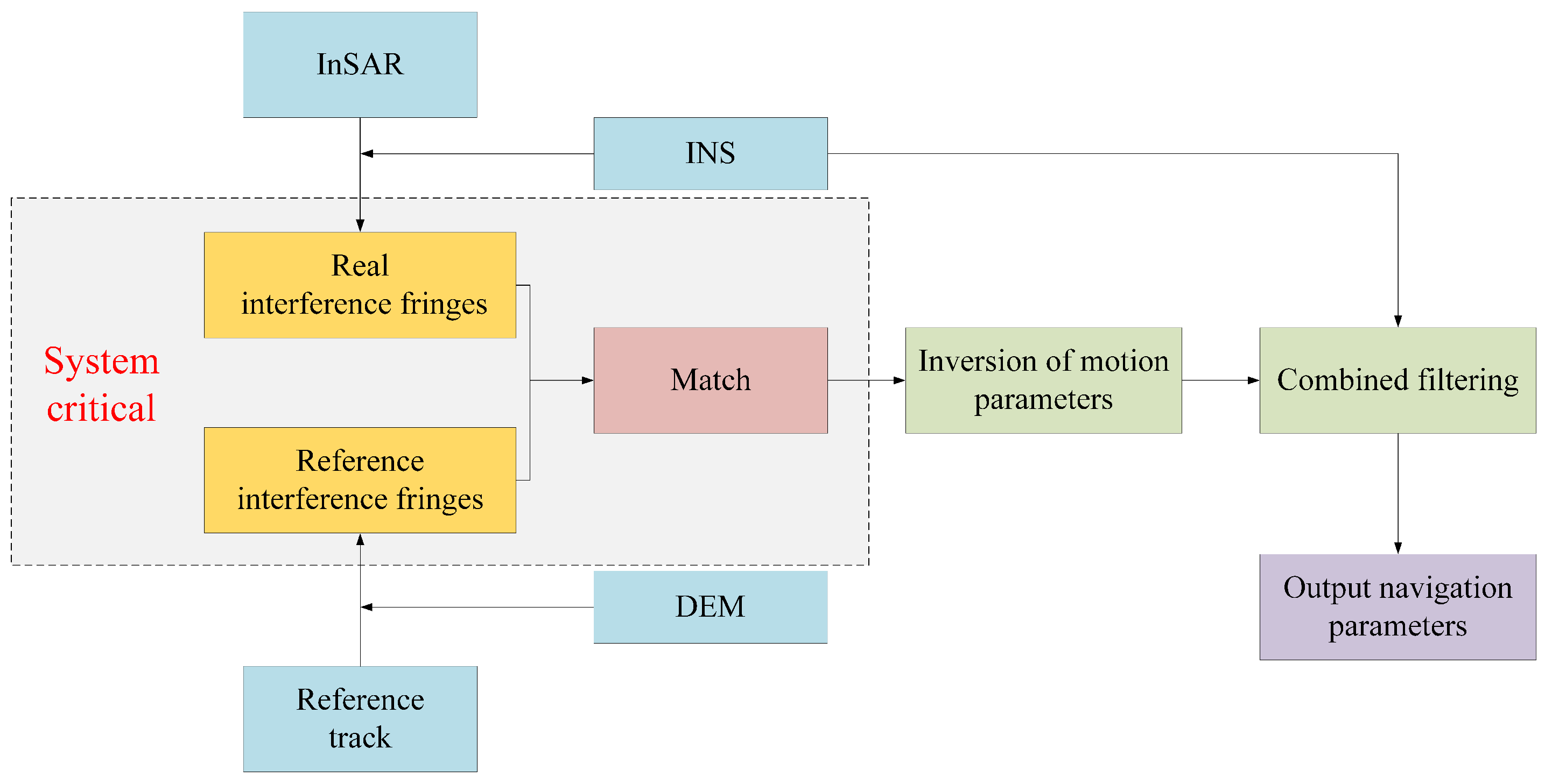
Figure 1. Framework of the interference fringe-matching navigation system.
Applsci 13 03941 g001
Figure 2. Algorithm flow.
Applsci 13 03941 g002
Figure 3. Interference phase versus elevation values. (a) InSAR system geometric model. (b) Simulation of the relationship between the interference phase and elevation value.
Applsci 13 03941 g003
Figure 4. Ridge detection in relation to edge detection. (a) Difference between the first derivative and second derivative. (b) Simulated ridge. (c) Edge detection. (d) Ridge detection.
Applsci 13 03941 g004
Figure 5. The process of extracting the mountain range line.
Applsci 13 03941 g005
Figure 6. Mountain line extraction results. (a) Interference fringe demonstration area. (b) Results of interference fringe mountain line extraction.
Applsci 13 03941 g006
Figure 7. Branch point detection template.
Applsci 13 03941 g007
Figure 8. Branch point extraction results. (ae) Real interference fringe. (fj) Reference interference fringe. (b,g) Valley line extraction results. (c,h) Valley branch point extraction results. (d,i) Ridge line extraction results. (e,j) Ridge branch point extraction results.
Applsci 13 03941 g008
Figure 9. Analysis of the influence of phase winding. (a) The demonstration area of interference fringes with phase winding. (b) Interference fringe eigenvalue map. (c) Slice 1, with calculation of the absolute value. (d) Slice 2.
Applsci 13 03941 g009
Figure 10. Verification of branch point detection algorithm. (a) Detection results of valley branch points of interference fringe with phase mutation. (b) Detection results of ridge branch points of interference fringe with phase mutation.
Applsci 13 03941 g010
Figure 11. Optimizing Gaussian functions using topography. (a) Gaussian function. (b) Mask of mountain line. (c) Improved Gaussian function. Branch point extraction results.
Applsci 13 03941 g011
Figure 12. Extraction descriptors.
Applsci 13 03941 g012
Figure 13. Comparison of improvement effects of descriptors. (a,b) Homonymous points of valley. (d,e) Homonymous points of ridge. (c,f) Euclidean distances of SIFT and the proposal descriptor.
Applsci 13 03941 g013
Figure 14. Experimental information. (a) Experimental site. (b) Radar and antenna. (c) DEM as well as longitude and latitude information corresponding to experimental data.
Applsci 13 03941 g014
Figure 15. Experimental data. (a) The corresponding SAR image of the experimental area. (b) Real interference fringe with noise. (c) Real interference fringe after noise removal. (d) Real interference fringe after removing the leveling effect.
Applsci 13 03941 g015
Figure 16. Reference interference fringe. (a) Reference interference fringe without errors. (b) Example of reference interference fringe with position errors. (c) Example of a reference interference fringe with attitude errors.
Applsci 13 03941 g016
Figure 17. Comparison of interference fringe-matching algorithm results in the position error experiment. (ac) Without error. (df) With error. (a,d) SIFT. (b,e) SURF. (c,f) Proposed algorithm.
Applsci 13 03941 g017
Figure 18. Quantitative comparison of interference fringe-matching algorithms in the position error experiment. (a) Precision. (b) Recall. (c) Inliers. (d) F1-Score.
Applsci 13 03941 g018
Figure 19. Comparison of interference fringe-matching algorithm results in the attitude error experiment. (a) SIFT. (b) SURF. (c) Proposed algorithm.
Applsci 13 03941 g019
Figure 20. Quantitative comparison of interference fringe-matching algorithms in the attitude error experiment. (a) Precision. (b) Recall. (c) Inliers. (d) F1-Score.
Applsci 13 03941 g020
Table 1. Simulation parameters.
λ /(cm)H/(m)B/(m) α /( )
2.07515000.50
Table 2. Flight parameters.
λ /(cm)H/(m)B/(m) α /( ) R min /(m) S a /(m) S r /(m)
3.1254876.3001.04845.6013618.3800.9760.681
Table 3. Average of the quantitative evaluation indicators in the position error experiment.
PrecisionRecallInliersF1-Score
SIFT0.0180.0197.8780.016
SURF0.0190.01615.7800.012
Proposed0.1030.12872.0240.144
Table 4. Average of the quantitative evaluation indicators in the attitude error experiment.
PrecisionRecallInliersF1-Score
SIFT0.0190.0198.2460.017
SURF0.0080.01510.8520.009
Proposed0.0930.11261.6550.108
Disclaimer/Publisher’s Note: The statements, opinions and data contained in all publications are solely those of the individual author(s) and contributor(s) and not of MDPI and/or the editor(s). MDPI and/or the editor(s) disclaim responsibility for any injury to people or property resulting from any ideas, methods, instructions or products referred to in the content.