Abstract
This study aims to develop PM2.5 prediction models using air pollutant data (PM10, NO2, SO2, O3, CO, and PM2.5) and meteorological data (temperature, humidity, wind speed, atmospheric pressure, precipitation, and snowfall) measured in South Korea from 2015 to 2019. Two prediction models were developed using an artificial neural network (ANN): a nationwide (NW) model and administrative districts (AD) model. To develop the prediction models, the independent variables daily averages and variances of air pollutant data and meteorological data (independent variables) were used as independent variables, and daily average PM2.5 concentration set as a dependent variable. First, the correlations between independent and dependent variables were analyzed. Second, prediction models were developed using an ANN to predict next-day PM2.5 daily average concentration, both NW and in 16 AD. The ANN models were optimized using a factorial design to determine the hidden layer layout and threshold, and a seasonal (monthly) factor was also considered. In the optimal prediction model, the absolute error in 1 σ was 91% (in-sample 91%, out-of-sample 91%) for the NW model, and the absolute error in 1 σ was 86% (in-sample 88%, out-of-sample 84%) for AD model. The accuracy of these prediction models increases further when they are developed using the next-day weather data, assuming that the weather prediction is accurate.
1. Introduction
Particulate matter (PM) is a global concern that is emitted locally and moves intercontinentally via long-range transport [1,2]. PM2.5 (particulate matter with an aerodynamic diameter smaller than 2.5 μm) can penetrate deep into the lungs and enter the bloodstream [3,4], which majorly affects the cardiovascular and respiratory systems [5] but also affects other organs. Exposure to air pollutants, including PM2.5, reportedly causes 7 million premature deaths every year [6], and can cause lung function decline [7,8], respiratory infections [9,10], and asthma [11,12] in vulnerable groups, such as children. In developing countries, air quality improvement is urgently required because of the unprotected use of fossil fuels [13,14]. In 2013, the International Agency for Research on Cancer (IARC) classified outdoor air pollution and PM2.5t as carcinogens [15]. In addition, in September 2021, the World Health Organization (WHO) lowered the new air quality guideline for PM2.5 to an annual average of 5 μg/m3 from 10 μg/m3, considering the effects of the particles on the human body due to long-term exposure [16]. An accurate PM2.5 daily prediction model help people plan their outdoor activities according to PM2.5. It will contribute to reducing the incidence of diseases caused by PM2.5 concentration. Therefore, a PM2.5 daily prediction model is developed in this study.
PM2.5 is mainly emitted directly by fuel combustion in various sectors including transportation, energy, household, industry, and agriculture [17,18]. It is also emitted in the form of nitrogen oxide (NOx) or sulfur oxide (SOx) during the gas phase reaction with ammonia (NH3) [19]. It is very difficult to control because it generates ammonium nitrate and ammonium sulfate, which are secondary PMs. Korea grapples with the effects of long-range transport as well as domestic emissions [20]. Although the concentration of PM2.5 in Korea is decreasing, remarkable long-lasting pollution episodes often occur, but remain difficult to predict. The National Institute of Environmental Research has been using a community multiscale air quality (CMAQ) model to predict the concentration of PM2.5 for air quality forecasting [21,22]. In the CMAQ model, meteorological and emission information are used as input data, although the accuracy of domestic and foreign emission information requires further improvement [23]. Korea forecasts PM2.5 by classifying it into four stages (low, moderate, high, and very high), and in 2018, the accuracy of the one-day and two-day forecasts were 73% and 68%, respectively; thus, uncertainty regarding these forecasts remains [24].
In recent years, air pollution prediction studies using artificial neural networks (ANN) have been widely conducted to improve the uncertainty of air quality prediction [25,26]. ANNs are used to accurately predict pollutant concentrations because they can build complex nonlinear models [27,28,29,30]. Various studies have been undertaken to predict dust concentrations. A study was conducted to forecast PM2.5 concentration by building a prediction model based on the radial basis function (RBF) neural network and comparing it with the existing back propagation (BP) network model [31]. Another study used particle swarm optimization (PSO) and fuzzy neural network as a more optimized method to predict PM2.5 concentration using meteorological factors and chemical composition of PM2.5. A case in which ANN technology was successfully applied to predict the concentration of PM2.5 in the air in a complex road traffic network was used to predict the concentration at a specific point [32]. To compensate for the disadvantages of CMAQ, Chang-hoi et al. conducted a study that grafted a recurrent neural network (RNN) to CMAQ [24,33]. However, most existing studies optimize the model or predict the concentration in a specific situation.
McKendry (2002) predicted next-day PM2.5 using ANN with today air pollutants’ (NOx, PM10, PM2.5, O3) concentrations and their variances and next-day precipitation and temperature as input variables [34]. Sun and Sun (2017) developed hybrid model next-day PM2.5 using PCA, LSSVM, and Cuckoo search [35]. The model developed in this study shows improved predictive performance compared to the models of the previous two studies and is presented in the results and discussion section. Among various ANN models, the multilayer perceptron artificial neural network in this study is a feedforward type ANN model that can be used universally, unlike the RBF, BP, PSO, and RNN-CMAQ mentioned above. Representatively, a PM2.5 prediction study using a multilayer perceptron artificial neural network predicted hourly PM2.5 using data from an hour ago using six measurement stations in Poland [36]. PM2.5 prediction studies using many ANNs, including the above studies, have focused only on hourly predictions, not daily predictions. Studies that predicted daily PM2.5 concentration by ANN are insufficient. In addition, when accurate weather forecasts are available, verification of performance changes of the forecasting model is not performed, so it is necessary to verify this.
Therefore, in this study, we developed a model that can predict each country nationwide and 16 administrative districts using ANN as a basic factor for air pollutant and meteorological data in Korea from 2015 to 2019. In addition, a one-day prediction model was developed, capable of next-day predictions of PM2.5 concentration if the air pollution and weather information of the day is known. In addition, models that could predict PM2.5 concentrations for NW and 16 administrative districts were developed using ANN.
2. Materials and Methods
2.1. Air Pollutants and Meteorological Data
In this study, as PM2.5 observation in South Korea began in 2015, air pollutant data and meteorological data from 2015 to 2019 were used. Operational details of instruments and their locations are provided elsewhere [37]. Air pollutant data were collected from 487 sites in 16 regions of Korea from 1 January 2015, to 31 December 2019, provided by Air Korea (https://www.airkorea.or.kr/, accessed on 1 October 2022) (operated by Korea Environment Corporation, Incheon, South Korea) [38]. These comprise the daily averages and daily variance data estimated using hourly data. Air pollutant factors (PM10, NO2, SO2, O3, CO, and PM2.5) were calculated with this data, which are daily averages and daily variances for nationwide (NW) and 16 administrative districts (AD; Seoul, Incheon, Gyunggi, Choongnam, Daejeon, Jeonbuk, GwangJu, Jeonnam, Gangwon, Choongbuk, Kyungbuk, Daegu, Ulsan, Kyungnam, Busam, and Jeju).
Meteorological data (temperature, humidity, wind speed, atmospheric pressure, precipitation, and snowfall) was provided by an automated synoptic observing system (ASOS) through Open Met Data Portal (https://data.kma.go.kr/, accessed on 1 October 2022) (operated by Korea Meteorological Administration, National Climate Data Center) [39]. The daily averages and variances were calculated for NW and AD based on 24 sites in the ASOS from 1 January 2015 to 31 December 2019. These daily average and variances were used as independent variables in the meteorological factors to predict next-day PM2.5 concentration.
2.2. Artificial Neural Networks
In this study, models to predict the next-day PM2.5 daily average for NW and AD were developed using an ANN. To develop prediction models using ANN, R version 4.1.0 was used with the “neuralnet” library. The variables in Table 1 were used to develop the models; y was used as a dependent variable, while the rest were used as independent variables.

Table 1.
Variables for prediction model development.
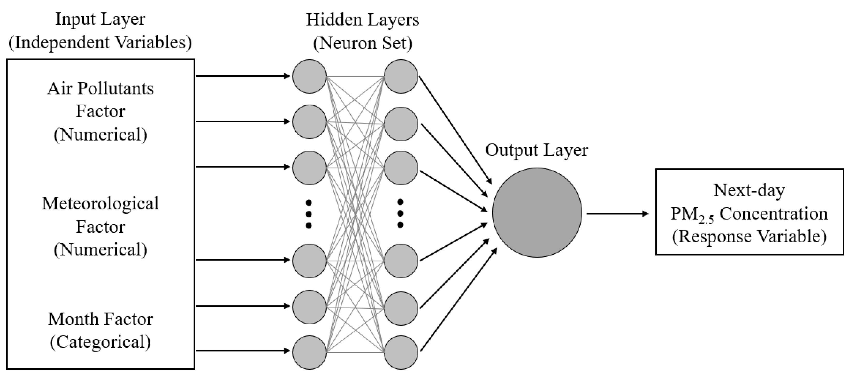
PM2.5 prediction model was developed separately for NW and AD. All independent variables are connected to the neurons in the hidden layer, which is composed of two columns, as shown in Figure 1. These neurons pass through the activation function and produce an output. In this study, a Logistic Function, Equation (1), was used as the activation function. Therefore, an optimal function is obtained when the neuron inputs are between 0 and 1, and the numerical independent variables of air pollutants and meteorological factors are converted into data between 0 and 1 through the min–max normalization of Equation (2) [40].

Figure 1.
Scheme of the artificial neural network model.
The value that has passed through the neurons of the hidden layer is gathered in the output layer and calculated, and a response variable is subsequently derived. The error between the predicted and actual values is reduced, and the model is repeatedly learned. A model is learned to allow the partial derivative of the sum of squared error (SSE), which is the error function for the difference between the predicted and actual values derived from the model, to become smaller than the threshold [41]. This method is known as the “Rprop+” algorithm. Model learning is terminated when the absolute partial differential value of the SSE becomes smaller than the specified threshold or when the set number of training reaches 106 [42].
ANN showed high prediction performance for time-series prediction in previous studies, but the ANN model could not entirely explain the relationship between the dependent and independent variables [43]. Therefore, the developed model should be verified using data not employed for model development. Two-thirds of the total data were used for model development (called “in-sample”) and the remaining data (called “out-of-sample”) were used for model validation. Two-thirds of each comprehensive air quality index category (good, normal, bad, and very bad) were randomly extracted and used as an in-sample (Tables S1 and S2). The decision to use a monthly factor to account for seasonal patterns affected the accuracy of the model. In addition, in Figure 1, the number of nodes and the number of hidden layers are shown, and this combination is called the hidden layer layout. The hidden layer layout should be optimized for best performance [44]. In addition, an appropriate threshold must be determined to prevent model overfitting. Table 2 shows the level of the factors used to determine the optimal ANN model. The presence or absence of the month factor, hidden layer layout, and threshold were tested and analyzed using a factorial design.

Table 2.
Levels of factorial design for artificial neural network model optimization.
In the pre-experiment, at least three layers showed no significant performance improvement, and the use of one layer was not appropriate for the ANN [45]. Therefore, the number of layers was fixed at two (Table 2). The hidden layer layout is expressed as two, that is, n × n. The first n is the number of nodes in the first layer, and the second n is the number of nodes in the second layer. Generally, the number of nodes in each layer is the total number of independent variables or [log]2 (the number of independent variables) [46,47]. Therefore, the factor level was set by reducing it by half from 24, which is the sum of 12 (total number of air pollutant factors) and 12 (total number of meteorological factors). The threshold value was found to overfit when the default value of R (0.01) was used. To prevent overfitting, the threshold values were tested with default values of 0.01, five times the default value of 0.05, and 10 times the default value of 0.1.
Eighteen (2×3×3) prediction models each for NW and AD were developed according to the level combination of the parameters in Table 2 using in-sample and verified by out-of-sample. Detailed model performance and verification results are presented in the next section.
2.3. Model Validation Metrics
To evaluate the performance of the prediction models, ‘R-squared’ and ‘absolute errors in n σ’ were used as model validation metrics. The absolute error in n σ’ is shown in Equation (3). First, the absolute errors between the actual measured value of PM2.5, , and the predicted value of PM2.5, were calculated. Second, the percentage of absolute errors, , that fell within n σ were calculated. The closer the absolute error of n σ’ is to 1, the more accurate the predictive model.
The standard of ‘Absolute Error in n σ’ is determined based on the standard deviation of PM2.5. For a conservative judgment, 1 σ (standard deviation) was set to 12. As shown in Table 3, the same threshold of ‘absolute error in n σ’ was set for both NW and AD.

Table 3.
Absolute error threshold for n σ.
3. Results and Discussion
3.1. Trend and Correlation Analysis for Input Parameter
Table 4 displays the basic statistics of air pollutant factors for nationwide and administrative districts. Based on these, Table 4 and the South Korea comprehensive air quality index (Table S1), PM10 and PM2.5 have normal levels on an average, whereas NO2, SO2, O3, and CO show good concentrations. However, the maximum values in Table 4 show harmfully high levels of PM10 and PM2.5, and bad levels of NO2 and O3 depending on the region. Table S2 provides in-depth details of the PM2.5 factor, which is the response variable in this study. Over 80% of PM2.5 daily averages were good or normal, whereas very bad concentrations were scarce.

Table 4.
Statistical description of daily air pollutant factor, 2015–2019.
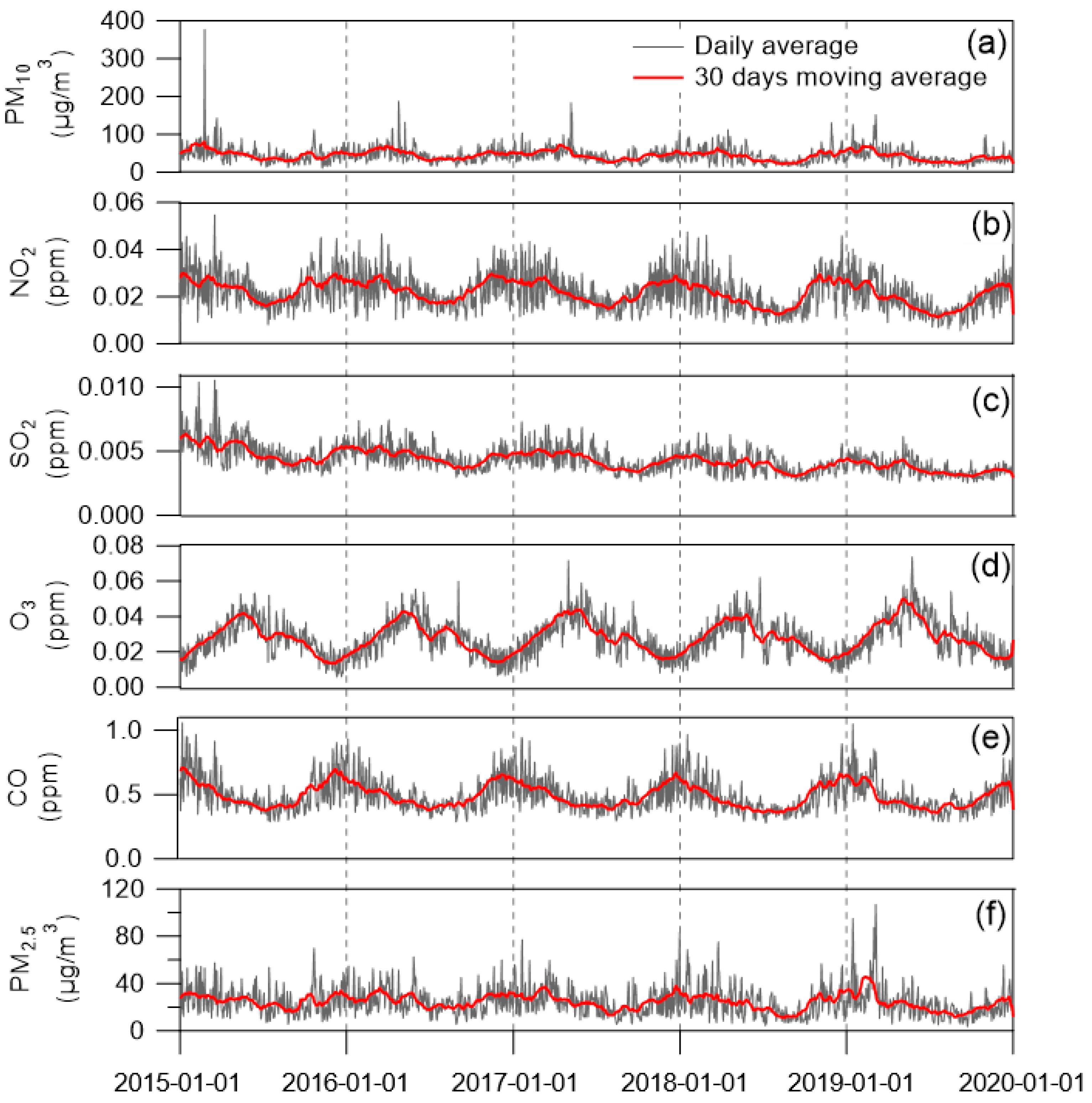
Figure 2 shows the daily average of air pollutant data and the 30-day moving average of the daily average. Each air pollutant factor had a seasonal pattern; PM10, NO2, SO2, and CO showed a decreasing trend every year, whereas O3 showed an increasing trend. PM10 was high in the winter and low in the summer. NO2, SO2, and CO also show patterns similar to those of PM10. PM2.5 also shows a similar pattern to PM10, as shown in Figure 2. Conversely, O3 was high in summer and low in winter.
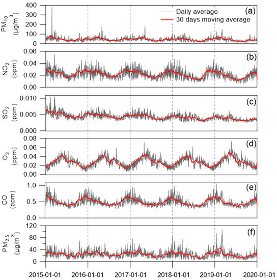
Figure 2.
Daily average and 30−day moving average for (a) PM10, (b) NO2, (c) SO2, (d) O3, (e) CO, and (f) PM2.5.
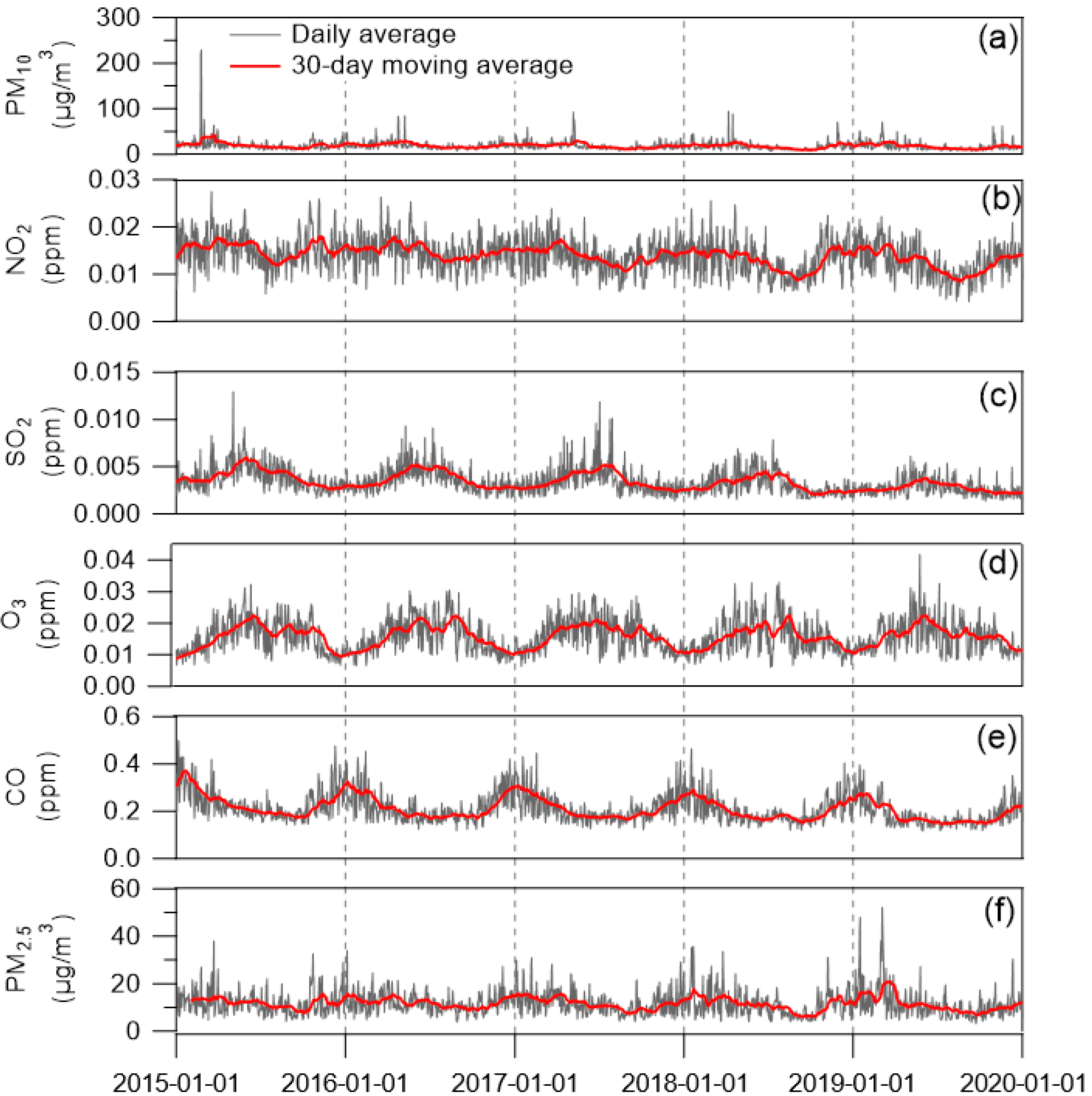
Figure 3 shows the daily standard deviation of the air pollutant data and its 30-day moving average. A seasonal pattern in the standard deviation was also observed. As shown in Figure 3, the daily standard deviation of PM2.5 varies seasonally, and the variance is large in winter and small in summer. As for NO2, SO2, and CO, the standard deviation in summer decreases each year. As shown in Figure 3 and, CO concentration and its standard deviation are high in winter, low in summer, and decreases every year. As shown in Figure 3, the standard deviation of O3 was large in summer and small in winter. As shown in Figure 2 and Figure 3, PM10, O3, CO, and PM2.5, all had large standard deviations when the daily average was high and small standard deviations when the daily average was low.
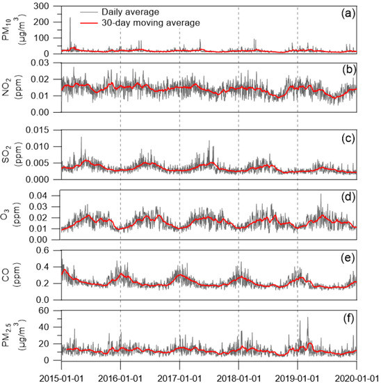
Figure 3.
Daily standard deviation and 30−day moving average for (a) PM10, (b) NO2, (c) SO2, (d) O3, (e) CO, and (f) PM2.5.
Table 5 presents the basic statistics of the meteorological factors, where precipitation indicates the amount of rain per hour, and snowfall indicates the height of snow accumulation from the hourly indicator. Therefore, the daily average snowfall represents the average daily snow height from the ground. In the case of the daily average snowfall, there was a significant difference between administrative districts. Precipitation and snowfall were not observed meteorological phenomena due to the characteristics of the factor; therefore, the days when they do not occur have a value of 0, and the value of median is 0 or close to 0 because precipitation and snowfall are not observed for over half of the year.

Table 5.
Statistical description of daily meteorological factor, 2015–2019.
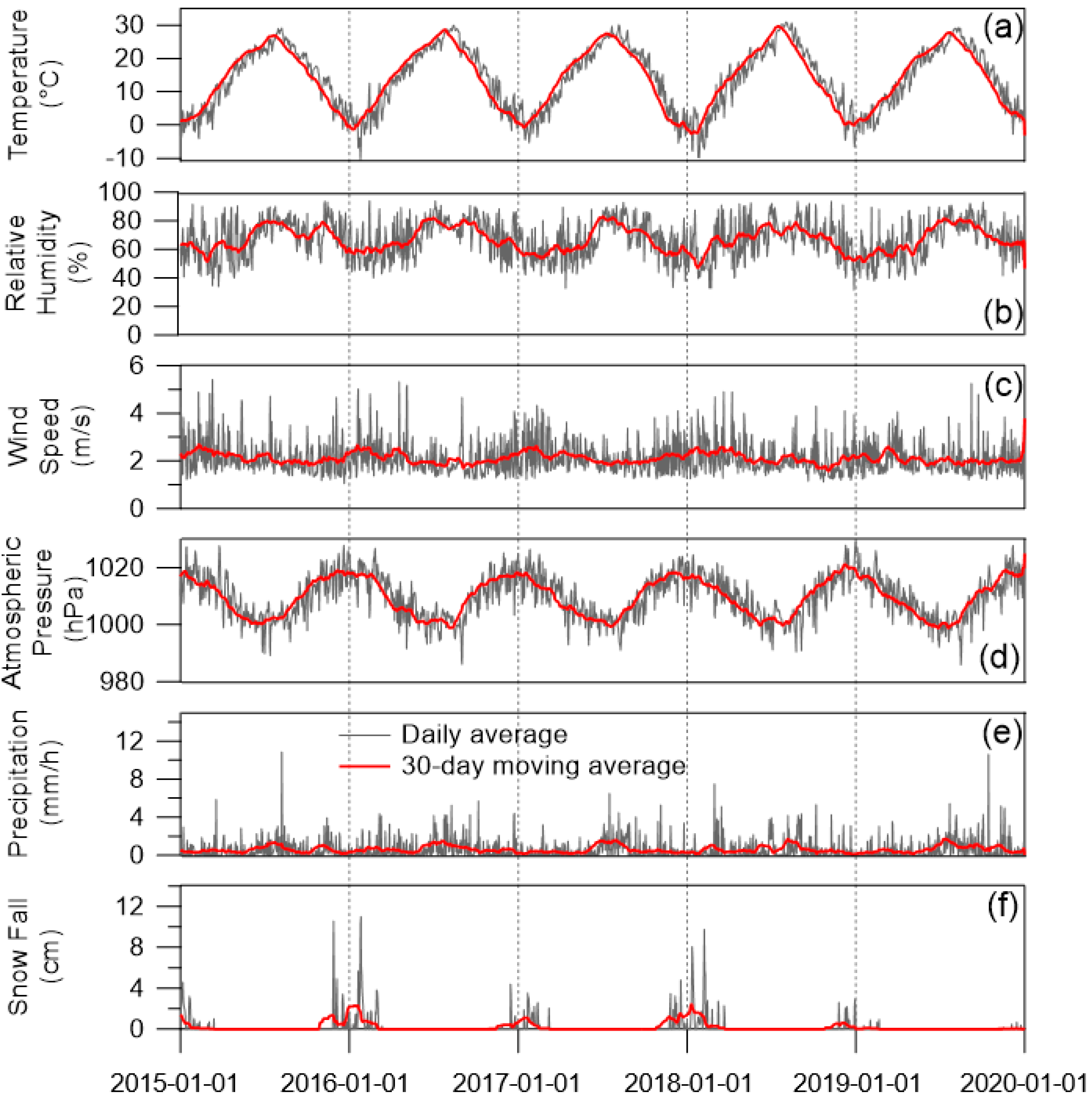
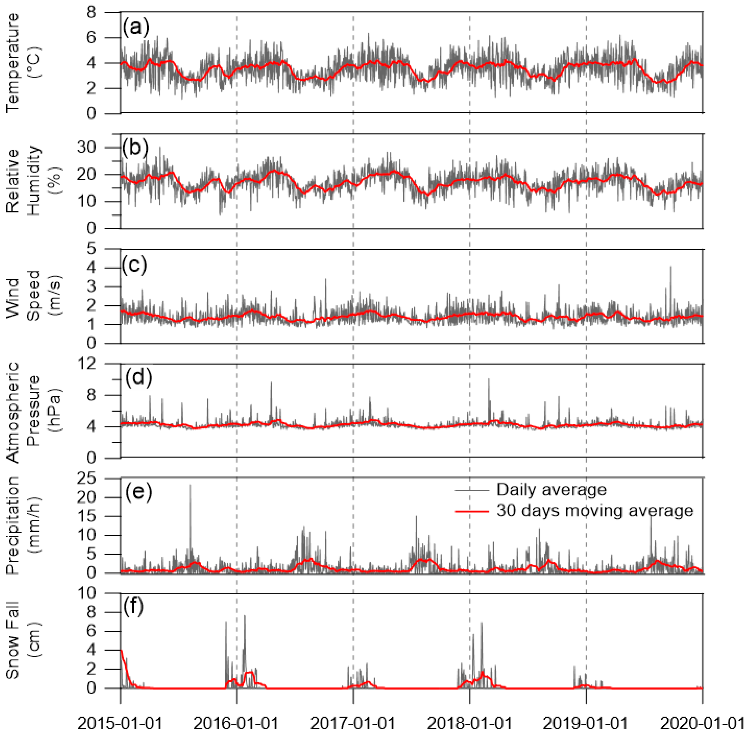
Figure 4 shows the daily average and 30-day moving average of the meteorological data. Each meteorological factor exhibited a seasonal pattern. Temperature, humidity, and precipitation were high in summer and low in winter, and from the wind speed and atmospheric pressure are high in winter and low in summer. Snowfall is observed in winter due to its seasonal characteristics.
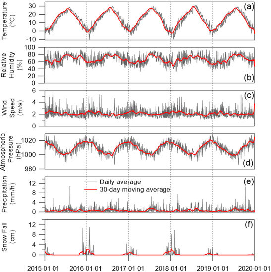
Figure 4.
Daily average with 30−day moving average for (a) Temperature, (b) Relative humidity, (c) Wind speed, (d) Atmospheric pressure, (e) Precipitation, and (f) Snow fall.
Figure 5 shows the daily standard deviation of the meteorological data and 30-day moving average. In the standard deviation, seasonal patterns similar to the daily average patterns were observed. As shown in Figure 5, the standard deviations of temperature, humidity, wind speed, and atmospheric pressure are small in summer and large in winter, and the standard deviation in precipitation is large in summer and small in winter. Snowfall is observed exclusively in winters, the standard deviation appears only during winter.
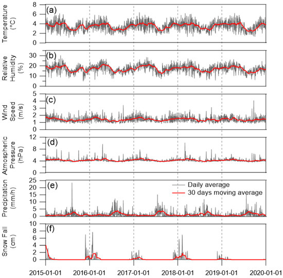
Figure 5.
Daily standard deviation with 30−day moving average for (a) Temperature, (b) Relative humidity, (c) Wind speed, (d) Atmospheric pressure, (e) Precipitation, and (f) Snow fall.
Because the air pollutant factor is known to affect the occurrence of PM2.5 and meteorological factors reflect seasonal changes, they are appropriate as independent variables in the prediction of PM2.5. To examine their relationship in greater depth, the correlation between the air pollutants and meteorological factors and the next-day PM2.5 concentration was analyzed. Independent and dependent variables used to develop the prediction model are summarized in Table 1. Air pollutant and meteorological factors were independent variables, and next-day PM2.5 concentration was the dependent variable to be predicted. As correlations using NW data and AD data are very similar, only the correlation with NW data is presented.
Results of correlation analysis for next-day PM2.5 and air pollutant factors are summarized in Table 6. The daily average concentrations of PM10 (0.57), NO2 (0.62), SO2 (0.52), CO (0.63), and PM2.5 (0.71), which are air pollutants excluding O3 (−0.02), showed a high positive correlation with next-day PM2.5. In addition, next-day PM2.5 had a positive correlation with the variances of the air pollutants, and had a positive correlation with NO2 (0.58), CO (0.46), and PM2.5 (0.49). Based on the correlation analysis results, using daily variances of air pollutants as independent variables is, thereby, reasonable.

Table 6.
Correlations among next-day PM2.5 and air pollutants (nationwide daily average and variance).
Table 7 shows the correlation between next-day PM2.5 and meteorological factors. In terms of the daily average, next-day PM2.5 was positively correlated with atmospheric pressure (0.29) and snowfall (0.05). Temperature (−0.31), humidity (−0.21), wind speed (−0.32), and precipitation (−0.26) were negatively correlated with next-day PM2.5. In terms of daily variance, next-day PM2.5 was positively correlated with temperature (0.40), humidity (0.30), and snowfall (0.02), and negatively correlated with the rest of the factors. In general, meteorological factors had lower correlations than air pollutant factors but were used for prediction model development as important independent variables showing seasonal changes.

Table 7.
Correlations among next-day PM2.5 levels and meteorological factors (nationwide daily average and variance).
3.2. PM2.5 Prediction Model for Nationwide
According to the factor levels in Table 2, 18 prediction models were developed NW. Table 8 shows the analysis of variance (ANOVA) table that statistically explains the factorial design experiment results. The response variable in this table is the R-squared of the out-of-sample. Based on a significance level of 0.05, all main effects (hidden layer layout, month, and threshold) affected R-squared. Two interaction effects (month factor and hidden layer layout, and hidden layer layout and threshold) also affected R-squared. Therefore, three factors affected the predictive model. This shows that it is appropriate to find the optimal model according to level change.

Table 8.
ANOVA table of nationwide PM2.5 prediction model.
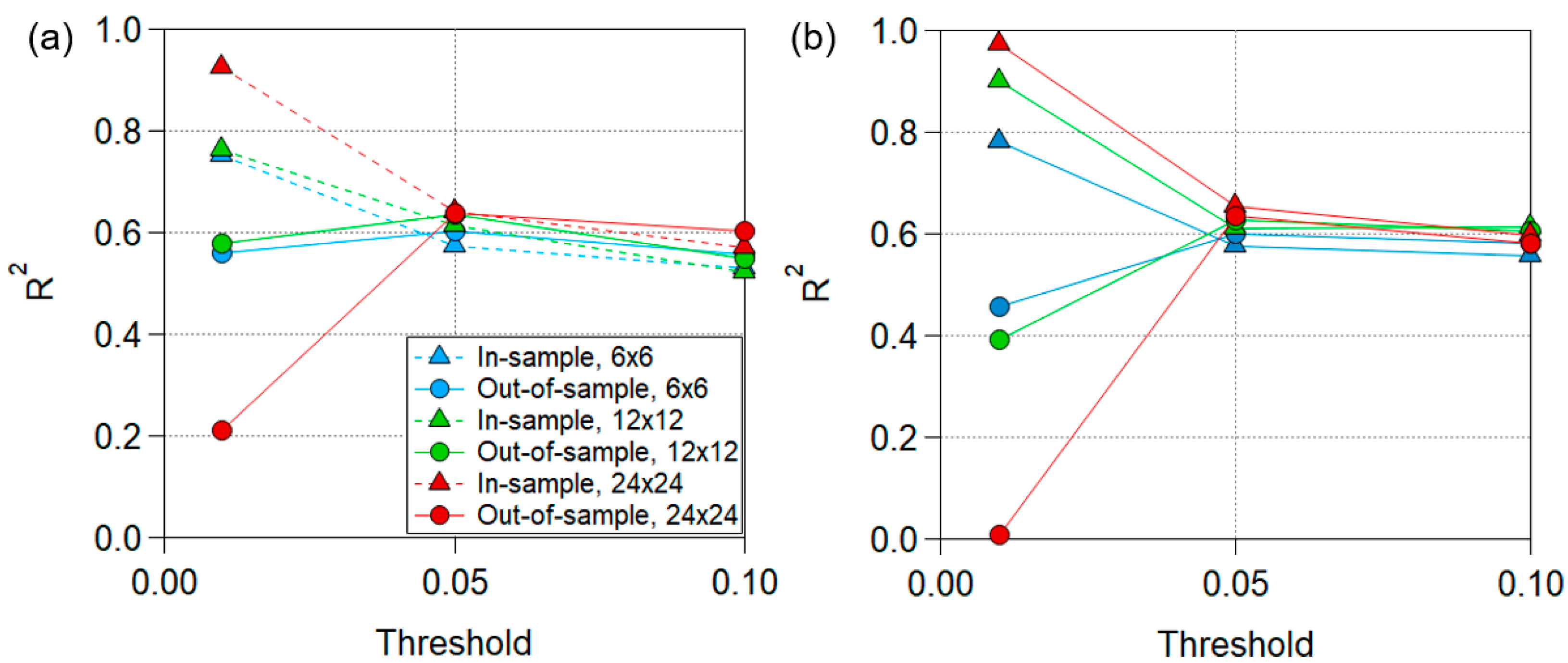
Figure 6a,b show in-sample/out-of-sample R-squared of the 18 prediction models developed according to factorial design, respectively. The higher the R-squared value was, the better the predictive ability of the model was. However, to avoid overfitting, the difference in R-squared between in-sample and out-of-sample should be minimal. Thus, to prevent overfitting, the model with a high average R-squared (average R-squared for in-sample and out-of-sample) was selected as the optimal model among the models in which the in-sample and out-of-sample R-squared differed within 10%. Using the month factor showed higher R-squared, and in-sample R-squared decreased as the threshold increased. However, if the threshold increased from 0.01 to 0.05 or 0.1, the deviation of R-squared between in-sample and out-of-sample decreased, thereby reducing the overfitting problem. Therefore, with the overfitting problem reduced, the model with the highest average R-squared (month factor: included, hidden layer layout: 24 × 24, threshold: 0.05) was determined as the optimal model. Assuming that the weather prediction is accurate, if the meteorological factor on the forecasting day is used instead of data from the previous day, the R-squared increased from 0.65 to 0.81 for in-sample and from 0.64 to 0.73 for out-of-sample as shown in Table 9. The absolute error n σ also increased, indicating that the accuracy of the model could be further improved if accurate weather predictions were used.
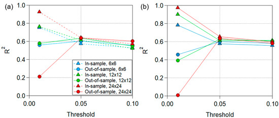
Figure 6.
R-squared for nationwide models: (a) excluding month factor and (b) including month factor.

Table 9.
R-squared and absolute errors in n σ of nationwide model with/without accurate weather forecasting (Month factor: included, hidden layer layout: 24 × 24, threshold: 0.05).
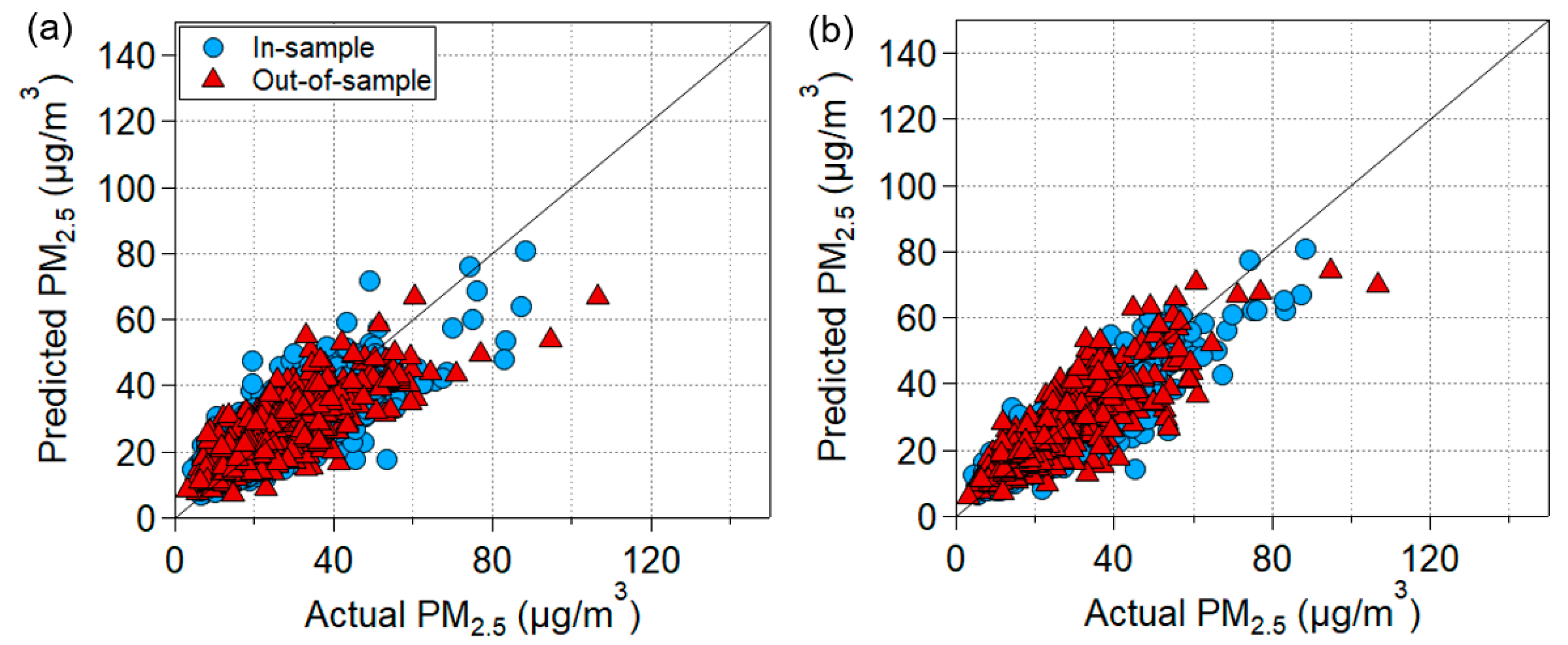
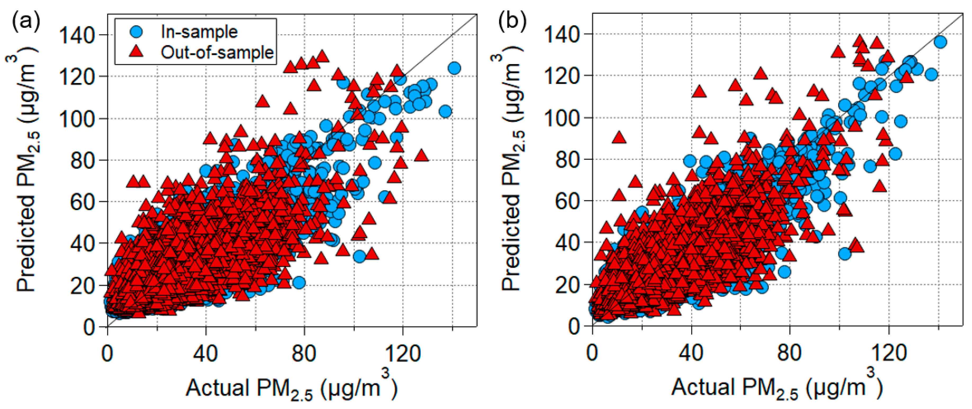
The predicted and actual values of the optimal prediction model are presented in Figure 7. The distribution of most of the results proximate to the centerline indicates that the model adequately predicted PM2.5. Figure 7b has a slightly smaller difference between the predicted and the measured values than Figure 7a.
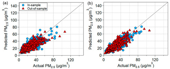
Figure 7.
PM2.5 prediction vs. actual PM2.5 for nationwide model: (a) not considering accurate weather prediction and (b) considering accurate weather prediction.
3.3. PM2.5 Prediction Model for Administrative Districts
The PM2.5 prediction model for AD, was developed in the same way as the NW PM2.5 prediction model. As shown in Table 10, based on a significance level of 0.05, the two main effects of the hidden layer layout and the threshold were significant, and they were also the most significant among all the interaction effects. Unlike the NW analysis, the month factor was not clearly significant in the ANOVA.

Table 10.
ANOVA table of PM2.5 prediction model for administrative districts.
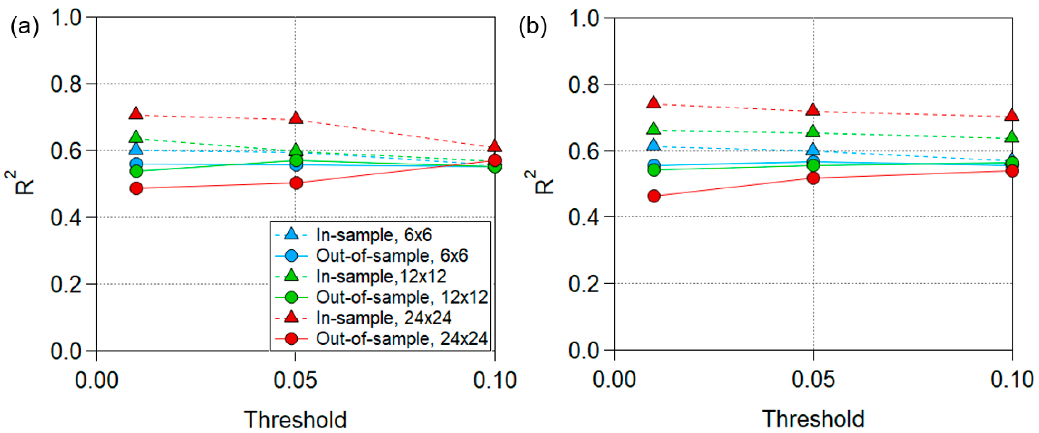
As with the NW prediction model, the model with the month factor had higher overall R-squared than the model without the month factor (Figure 8). Although it is not as sharp as the NW model in Figure 6, the in-sample R-squared value decreased as the threshold increased. As the number of nodes in the hidden layer layout decreased and the threshold increased, Figure 8 describes that the deviation between the in-sample and out-of-sample R-squared values decreased, and the overfitting problem also reduced. Therefore, the model with the highest average R-squared value and a less than 10% difference between in-sample and out-of-sample R-squared values was selected as the optimal PM2.5 prediction model. Thus, when the month factor was included, the number of nodes in the hidden layer layout was 12, and the threshold was 0.05.
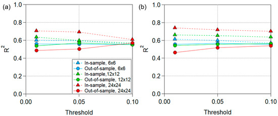
Figure 8.
R-squared for administrative district model: (a) excluding month factor and (b) including month factor.
Table 11 shows the R-squared and absolute errors in n σ of the optimal PM2.5 prediction model for AD (month factor: included, hidden layer layout: 6 × 6, threshold: 0.05). As shown in Figure 8 and Table 5, the accuracy of the PM2.5 prediction model for AD is slightly lower than that of the PM2.5 NW prediction model. R-squared of PM2.5 prediction model without weather forecasting for AD are 0.65 (in-sample) and 0.55 (out-of-sample), and the absolute error in 1 σ is 88% and 84%, respectively. Assuming that the weather prediction is accurate, if the meteorological factor on the forecasting day is used instead of data from the previous day, The R squared increased from 0.65 to 0.73 for in-sample and from 0.55 to 0.65 for out-of-sample. The accuracy of the NW PM2.5 prediction model can be improved with high accuracy weather forecasting.

Table 11.
R-squared and absolute errors in n σ of administrative district model with/without accurate weather forecasting (month: included, hidden layer layout: 12 × 12, threshold: 0.05).
Figure 9 presents the predicted and measured values of the optimal PM2.5 prediction model for the AD. PM2.5 in each region is accurately predicted without considering regional variables. Figure 9b has a slightly smaller difference between the predicted and measured values than Figure 9a. In future studies, a regional variable should be considered or a regional model should be developed separately to further improve the predictive power of the model.
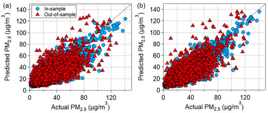
Figure 9.
PM2.5 prediction vs. actual PM2.5 for the administrative district model: (a) not considering accurate weather prediction and (b) considering accurate weather prediction.
Next-day PM2.5 prediction models are compared in Table 12. The PM2.5 prediction model developed in this study is superior to the two preceding studies in terms of R-squared and mean absolute error (MAE). However, since the data used in each study is different, it may be inappropriate to compare only R-squared and MAE.

Table 12.
Next-day PM2.5 prediction model performance comparison.
4. Conclusions
In this study, the correlation between the daily averages and daily variances of air pollutants and meteorological factors was analyzed with next-day PM2.5 concentrations. Through this, it was confirmed that next-day PM2.5 concentration was not only influenced by the daily average of air pollutant data and meteorological data but also by the daily variances.
The data were divided into two types: NW data and administrative district data (16 regions). Subsequently, daily averages and variances of air pollutant data (PM10, NO2, SO2, O3, CO, and PM2.5) and meteorological data (temperature, humidity, wind speed, atmospheric pressure, precipitation, and snowfall) were calculated. A prediction model that determined next-day PM2.5 was developed using an ANN. Factorial design was used to find the best factor level (month, hidden layer layout, and threshold) for the ANN, and the optimal model was selected based on ANOVA. The absolute error in 1 σ of the PM2.5 NW prediction model is 91% (in-sample 91%, out-of-sample 91%), and that for AD is 86% (in-sample 88%, out-of-sample 84%). Assuming that the weather forecast was accurate, the accuracy of these prediction models (absolute error in 1 σ) increased up to 96% (in-sample) and 92% (out-of-sample) for NW and 91% (in-sample) and 89% (out-of-sample) for the AD.
Our developed model has a significant advantage over traditional predictive models in that it uses the air pollutions and meteorological data of the current day to forecast the PM2.5 for the next day. This is more convenient than conventional models that rely on statistical analysis or air pollution modeling, such as CMAQ. Regions such as South Korea, where haze events are common, experience daily PM2.5 concentration fluctuations of more than three times during the event [19]. As a result, it is crucial to have a model that can provide people with an action plan to prepare for these daily changes. Our study confirmed the accuracy of the NW model, and we plan to conduct an optimization study of the AD model, which is relatively inaccurate, in future research.
Supplementary Materials
The following supporting information can be downloaded at: https://www.mdpi.com/article/10.3390/app13063575/s1, Table S1. Concentration ranges of air pollutants, comprehensive air quality index in South Korea. Table S2. Number of data and % of each category for PM2.5. categorized by comprehensive air quality index in South Korea.
Author Contributions
Conceptualization, S.P.; methodology, J.-W.H.; software, J.-W.H. and P.-M.P.; validation, J.-W.H. and J.-S.Y.; formal analysis, J.-W.H.; investigation, K.-J.J.; resources, S.P.; data curation, S.P.; writing—original draft preparation, J.-W.H. and J.-S.Y.; writing—review and editing, S.P. and K.-J.J.; visualization, J.-S.Y.; supervision, S.P. and K.-J.J.; project administration, S.P. and K.-J.J.; funding acquisition, S.P. All authors have read and agreed to the published version of the manuscript.
Funding
This study was supported by a 2021 Research Grant from Kangwon National University. This work was also supported by a grant from the National Institute of Environment Research (NIER), funded by the Ministry of Environment (MOE) of the Republic of Korea (NIER-2021-03-03-007).
Institutional Review Board Statement
Not applicable.
Informed Consent Statement
Not applicable.
Data Availability Statement
Not applicable.
Acknowledgments
Thankful for support by a 2021 Research Grant from Kangwon National University and grant from the National Institute of Environment Research (NIER), funded by the Ministry of Environment (MOE) of the Republic of Korea.
Conflicts of Interest
The authors declare no conflict of interest.
References
- Kim, K.H.; Kabir, E.; Kabir, S. A review on the human health impact of airborne particulate matter. Environ. Int. 2015, 74, 136–143. [Google Scholar] [CrossRef]
- Wang, Z.; Itahashi, S.; Uno, I.; Pan, X.; Osada, K.; Yamamoto, S.; Nishizawa, T.; Tamura, K.; Wang, Z. Modeling the long-range transport of particulate matters for january in East Asia using NAQPMS and CMAQ. Aerosol Air Qual. Res. 2017, 17, 3065–3078. [Google Scholar] [CrossRef]
- Lee, P.H.; Park, S.; Lee, Y.G.; Choi, S.M.; An, M.H.; Jang, A.S. The impact of environmental pollutants on barrier dysfunction in respiratory disease. Allergy Asthma Immunol. Res. 2021, 13, 850. [Google Scholar] [CrossRef]
- Rosman, P.S.; Samah, M.A.A.; Yunus, K.; Hussain, M.R.M. Particulate matter (PM 2.5) at construction site: A review. Int. J. Recent Technol. Eng. 2019, 8, 255–259. [Google Scholar]
- Hamanaka, R.B.; Mutlu, G.M. Particulate Matter Air Pollution: Effects on the Cardiovascular System. Front. Endocrinol. 2018, 9, 68. [Google Scholar] [CrossRef]
- WHO. WHO|Air Pollution; World Health Organization: Geneva, Switzerland, 2019. [Google Scholar]
- Zwozdziak, A.; Sówka, I.; Willak-Janc, E.; Zwozdziak, J.; Kwiecińska, K.; Balińska-Miśkiewicz, W. Influence of PM1 and PM2.5 on lung function parameters in healthy schoolchildren—A panel study. Environ. Sci. Pollut. Res. 2016, 23, 23892–23901. [Google Scholar] [CrossRef]
- Yang, M.; Guo, Y.M.; Bloom, M.S.; Dharmagee, S.C.; Morawska, L.; Heinrich, J.; Jalaludin, B.; Markevychd, I.; Knibbsf, L.D.; Lin, S.; et al. Is PM1 similar to PM2.5? A new insight into the association of PM1 and PM2.5 with children’s lung function. Environ. Int. 2020, 145, 106092. [Google Scholar] [CrossRef]
- Bonyadi, Z.; Ehrampoush, M.H.; Ghaneian, M.T.; Mokhtari, M.; Sadeghi, A. Cardiovascular, respiratory, and total mortality attributed to PM2.5 in Mashhad, Iran. Environ. Monit. Assess. 2016, 188, 570. [Google Scholar] [CrossRef]
- Sherris, A.R.; Begum, B.A.; Baiocchi, M.; Goswami, D.; Hopke, P.K.; Brooks, W.A.; Luby, S.P. Associations between ambient fine particulate matter and child respiratory infection: The role of particulate matter source composition in Dhaka, Bangladesh. Environ. Pollut. 2021, 290, 118073. [Google Scholar] [CrossRef]
- Paterson, C.A.; Sharpe, R.A.; Taylor, T.; Morrissey, K. Indoor PM2.5, VOCs and asthma outcomes: A systematic review in adults and their home environments. Environ. Res. 2021, 202, 111631. [Google Scholar] [CrossRef]
- Vu, B.N.; Tapia, V.; Ebelt, S.; Gonzales, G.F.; Liu, Y.; Steenland, K. The association between asthma emergency department visits and satellite-derived PM2.5 in Lima, Peru. Environ. Res. 2021, 199, 111226. [Google Scholar] [CrossRef]
- Sharma, S.K.; Mandal, T.K.; Sharma, A.; Jain, S. Saraswati Carbonaceous Species of PM2.5 in Megacity Delhi, India During 2012–2016. Bull. Environ. Contam. Toxicol. 2018, 100, 695–701. [Google Scholar] [CrossRef]
- Khan, Z.Y.; Kettler, J.; Khwaja, H.A.; Naqvi, I.I.; Malik, A.; Stone, E.A. Organic aerosol characterization and source identification in Karachi, Pakistan. Aerosol Air Qual. Res. 2018, 18, 2550–2564. [Google Scholar] [CrossRef]
- IARC. IARC Monographs on the Evaluation of Carcinogenic Risks to Humans: Outdoor Air Pollution; IARC: Lyon, France, 2015; Volume 109, ISBN 9789283201755. [Google Scholar]
- WHO. WHO Global Air Quality Guidelines; Coastal and Estuarine Process; WHO: Geneva, Switzerland, 2021; pp. 1–360. [Google Scholar]
- Kim, I.; Lee, K.; Lee, S.; Kim, S.D. Characteristics and health effects of PM2.5 emissions from various sources in Gwangju, South Korea. Sci. Total Environ. 2019, 696, 133890. [Google Scholar] [CrossRef]
- Park, E.H.; Heo, J.; Kim, H.; Yi, S.M. Long term trends of chemical constituents and source contributions of PM2.5 in Seoul. Chemosphere 2020, 251, 126371. [Google Scholar] [CrossRef]
- Schlosser, J.S.; Stahl, C.; Sorooshian, A.; Le, Y.T.H.; Jeon, K.J.; Xian, P.; Jordan, C.E.; Travis, K.R.; Crawford, J.H.; Gong, S.Y.; et al. Evidence of haze-driven secondary production of supermicrometer aerosol nitrate and sulfate in size distribution data in South Korea. Atmos. Chem. Phys. 2022, 22, 7505–7522. [Google Scholar] [CrossRef]
- Kumar, N.; Park, R.J.; Jeong, J.I.; Woo, J.H.; Kim, Y.; Johnson, J.; Yarwood, G.; Kang, S.; Chun, S.; Knipping, E. Contributions of international sources to PM2.5 in South Korea. Atmos. Environ. 2021, 261, 118542. [Google Scholar] [CrossRef]
- Jeon, W.; Choi, Y.; Percell, P.; Hossein Souri, A.; Song, C.K.; Kim, S.T.; Kim, J. Computationally efficient air quality forecasting tool: Implementation of STOPS v1.5 model into CMAQ v5.0.2 for a prediction of Asian dust. Geosci. Model Dev. 2016, 9, 3671–3684. [Google Scholar] [CrossRef]
- Ho, C.H.; Park, I.; Kim, J.; Lee, J.B. PM2.5 Forecast in Korea using the Long Short-Term Memory (LSTM) Model. Asia-Pacific J. Atmos. Sci. 2022, 2022, 1–14. [Google Scholar] [CrossRef]
- Appel, K.W.; Napelenok, S.L.; Foley, K.M.; Pye, H.O.T.; Hogrefe, C.; Luecken, D.J.; Bash, J.O.; Roselle, S.J.; Pleim, J.E.; Foroutan, H.; et al. Description and evaluation of the Community Multiscale Air Quality (CMAQ) modeling system version 5.1. Geosci. Model Dev. 2017, 10, 1703–1732. [Google Scholar] [CrossRef]
- Chang-Hoi, H.; Park, I.; Oh, H.R.; Gim, H.J.; Hur, S.K.; Kim, J.; Choi, D.R. Development of a PM2.5 prediction model using a recurrent neural network algorithm for the Seoul metropolitan area, Republic of Korea. Atmos. Environ. 2021, 245, 118021. [Google Scholar] [CrossRef]
- Cheng, Y.; Zhang, H.; Liu, Z.; Chen, L.; Wang, P. Hybrid algorithm for short-term forecasting of PM2.5 in China. Atmos. Environ. 2019, 200, 264–279. [Google Scholar] [CrossRef]
- Wang, X.; Yuan, J.; Wang, B. Prediction and analysis of PM2.5 in Fuling District of Chongqing by artificial neural network. Neural Comput. Appl. 2021, 33, 517–524. [Google Scholar] [CrossRef]
- Ghosal, P.S.; Gupta, A.K. Enhanced efficiency of ANN using non-linear regression for modeling adsorptive removal of fluoride by calcined Ca-Al-(NO3)-LDH. J. Mol. Liq. 2016, 222, 564–570. [Google Scholar] [CrossRef]
- Polezer, G.; Tadano, Y.S.; Siqueira, H.V.; Godoi, A.F.L.; Yamamoto, C.I.; de André, P.A.; Pauliquevis, T.; Andrade, M.d.F.; Oliveira, A.; Saldiva, P.H.N.; et al. Assessing the impact of PM2.5 on respiratory disease using artificial neural networks. Environ. Pollut. 2018, 235, 394–403. [Google Scholar] [CrossRef]
- Dutta, A.; Jinsart, W. Air Pollution in Indian Cities and Comparison of MLR, ANN and CART Models for Predicting PM10 Concentrations in Guwahati, India. Asian J. Atmos. Environ. 2021, 15, 68–93. [Google Scholar] [CrossRef]
- Taylan, O.; Alkabaa, A.S.; Alamoudi, M.; Basahel, A.; Balubaid, M.; Andejany, M.; Alidrisi, H. Air quality modeling for sustainable clean environment using anfis and machine learning approaches. Atmosphere 2021, 12, 713. [Google Scholar] [CrossRef]
- Zou, B.; Wang, M.; Wan, N.; Wilson, J.G.; Fang, X.; Tang, Y. Spatial modeling of PM2.5 concentrations with a multifactoral radial basis function neural network. Environ. Sci. Pollut. Res. 2015, 22, 10395–10404. [Google Scholar] [CrossRef]
- Fang, M.; Zhu, G.; Zheng, X.; Yin, Z. Study on air fine particles pollution prediction of main traffic route using artificial neural network. In Proceedings of the International Conference on Computer Distributed Control and Intelligent Environmental Monitoring, CDCIEM 2011, Changsha, China, 19–20 February 2011. [Google Scholar]
- Lu, H.; Xie, M.; Wu, Z.; Liu, B.; Gao, Y.; Chen, G.; Li, Z. Adjusting PM2.5 prediction of the numerical air quality forecast model based on machine learning methods in Chengyu region. Huanjing Kexue Xuebao/Acta Sci. Circumstantiae 2020, 40, 4419–4431. [Google Scholar] [CrossRef]
- McKendry, I.G. Evaluation of artificial neural networks for fine particulate pollution (PM10 and PM2.5) forecasting. J. Air Waste Manag. Assoc. 2002, 52, 1096–1101. [Google Scholar] [CrossRef]
- Sun, W.; Sun, J. Daily PM2.5 concentration prediction based on principal component analysis and LSSVM optimized by cuckoo search algorithm. J. Environ. Manag. 2017, 188, 144–152. [Google Scholar] [CrossRef] [PubMed]
- Hoffman, S.; Jasiński, R. The Use of Multilayer Perceptrons to Model PM2.5 Concentrations at Air Monitoring Stations in Poland. Atmosphere 2023, 14, 96. [Google Scholar] [CrossRef]
- Youn, J.S.; Seo, J.W.; Park, W.; Park, S.; Jeon, K.J. Prediction model for dry eye syndrome incidence rate using air pollutants and meteorological factors in south korea: Analysis of sub-region deviations. Int. J. Environ. Res. Public Health 2020, 17, 4969. [Google Scholar] [CrossRef]
- Air Korea (Operated by Korea Environment Corporation). Available online: https://www.airkorea.or.kr (accessed on 21 January 2023).
- Open MET Data Poratal (Operated by Korea Meteorological Administration). Available online: https://data.kma.go.kr/ (accessed on 21 January 2023).
- Adeyemo, A.; Wimmer, H.; Powell, L.M. Effects of Normalization Techniques on Logistic Regression in Data Science. J. Inf. Syst. Appl. Res. 2020, 12, 89–104. [Google Scholar]
- Riedmiller, M.; Braun, H. RPROP—A Fast adaptive learning algorithm. In Proceedings of the Seventh International Symposium on Computer and Information Sciences, Santa Cruz, CA, USA, 22–25 June 1992. [Google Scholar]
- Günther, F.; Fritsch, S. Neuralnet: Training of neural networks. R J. 2010, 2, 30–38. [Google Scholar] [CrossRef]
- Papalambros, P.Y.; Wilde, D.J. Forecasting: Principles and Practice; OTexts: Melbourn, Australia, 2018. [Google Scholar]
- Stathakis, D. How many hidden layers and nodes? Int. J. Remote Sens. 2009, 30, 2133–2147. [Google Scholar] [CrossRef]
- Thomas, A.J.; Petridis, M.; Walters, S.D.; Gheytassi, S.M.; Morgan, R.E. Two hidden layers are usually better than one. In Proceedings of the Communications in Computer and Information Science, Athens, Greece, 25–27 August 2017. [Google Scholar]
- Wanas, N.; Auda, G.; Kamel, M.S.; Karray, F. On the optimal number of hidden nodes in a neural network. In Proceedings of the Canadian Conference on Electrical and Computer Engineering, Waterloo, ON, Canada, 25–28 May 1998. [Google Scholar]
- Shmueli, G.; Bruce, P.C.; Gedeck, P.; Patel, N.R. Data Mining for Business Analytics. Concepts, Techniques and Applications in Python; Wiley: Hoboken, NJ, USA, 2020; ISBN 9781119549840. [Google Scholar]
Disclaimer/Publisher’s Note: The statements, opinions and data contained in all publications are solely those of the individual author(s) and contributor(s) and not of MDPI and/or the editor(s). MDPI and/or the editor(s) disclaim responsibility for any injury to people or property resulting from any ideas, methods, instructions or products referred to in the content. |
© 2023 by the authors. Licensee MDPI, Basel, Switzerland. This article is an open access article distributed under the terms and conditions of the Creative Commons Attribution (CC BY) license (https://creativecommons.org/licenses/by/4.0/).

