Abstract
Efficient and low-cost modes for detecting metro track geometry defects (TGDs) are essential for condition-prediction-based preventive maintenance, which can help improve the safety of metro operations and reduce the maintenance cost of metro tracks. Compared with the traditional TGD detection method that utilizes the track geometry car, the method that uses a portable detector to acquire the car-body vibration data (CVD) can be used on an ordinary in-service train without occupying the metro schedule line, thereby improving efficiency and reducing the cost. A convolutional neural network-based identification model for TGD, built on a differentiable architecture search, is proposed in this study to employ only the CVD acquired by a portable detector for integrated identification of the type and severity level of TGDs. Second, the random oversampling method is introduced, and a strategy for applying this method is proposed to improve the poor training effect of the model caused by the natural class-imbalance problem arising from the TGD dataset. Subsequently, a comprehensive performance-evaluation metric (track geometry defect F-score) is designed by considering the actual management needs of the metro infrastructure. Finally, a case study is conducted using actual field data collected from Beijing Subway to validate the proposed model.
1. Introduction
Metro systems are an essential segment of modern large-scale urban transportation systems. In particular, the track is an essential part of the metro infrastructure, and maintaining optimal track quality guarantees safe train operation and comfortable passenger rides. Track geometry is the most widely used indicator of track quality and serves as the foundation for planning track maintenance activities [1]. This quality indicator is mainly represented by the following track geometry parameters: the longitudinal level (LL), alignment (AL), cross-level (CL), gauge (GA), and twist (TW) [2], as shown in Figure 1. Several countries have specified the management value of the deviation of track geometric parameters [3,4,5] and classified the deviation level according to management specifications [3,5]. In particular, a track geometry defect (TGD) reflects the state in which the track geometric parameter exceeds the management value. For example, in the field of urban rail transit in China, the deviation values of dynamic LLs are divided into four levels according to the national standard GB/T 39559.4-2020, and the management values are 12, 16, 22, and 26 mm [5]. According to the detection values of LL, severity levels of the defects can be determined based on these thresholds.
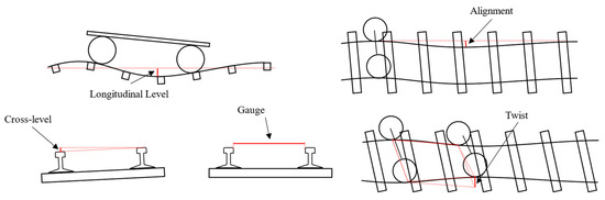
Figure 1.
Definition of track geometry parameters.
For a metro track, TGDs reduce the comfort of passengers and, in serious cases, affect the safety of train operation and may even lead to a train derailment. Thus, metro-operating companies employ various countermeasures for different defect severity levels according to actual management requirements [5,6]. As passenger demand for metro service quality is increasing, the metro-infrastructure management industry is gradually moving toward delicacy management, and condition-prediction-based preventive maintenance (CPM) for track geometry is gradually emerging as the mainstream technology. Thus, the foundation of CPM for track geometry is aimed at obtaining accurate and timely information concerning TGDs.
The most common method to detect dynamic TGDs involves the use of a track geometry car (TGC), which is a specialized full-scale track vehicle. The no-contact optical inertial-based track geometry measurement system is the principal tool used by a TGC to detect TGDs [7,8,9,10,11]. The system uses accelerometers, gyroscopes, and optical instruments installed on the TGC to measure the track geometry parameters. However, TGC-based detection involves high operating costs while offering a low detection frequency. For example, metro companies in China perform TGC detection every two months [5]. Therefore, the existing TGC-detection method cannot meet the delicacy management requirements of the metro-infrastructure management industry. In recent years, the metro industry has employed ordinary in-service trains for detecting TGDs. In particular, the technology of installing sensors [12,13] onto in-service trains or using portable sensing devices [14,15] to acquire vehicle vibration data [16] is used for detecting TGDs. This technology uses accelerometers and gyroscopes to collect data about the motions of various parts of the vehicle, which are used to estimate the track geometry condition [9,10,17]. Moreover, portable devices mounted in the cabin are more convenient and flexible to use for acquiring car-body vibration data (CVD) and reduce the need for sensor maintenance, which can further improve efficiency and reduce the cost of detection. However, a complex nonlinear relationship exists between CVD and TGD. Thus, using portable device-acquired CVD to identify TGDs is a difficult task in field applications, and this strategy is currently in the preliminary stages of development. Thus, the detection accuracy and applicable defect types should be further researched.
The main contributions of this study include the following: (1) a metro TGD identification convolutional neural network (CNN) model based on differential architecture search (DARTS) is proposed, which realizes the integrated identification of the type and severity level of TGD, (2) a strategy for coping with the class-imbalance problem of the dataset when modeling CNN models for TGD identification is proposed, which reduces the impact of the natural feature of the class-imbalance problem of the CVD–TGD dataset—a drawback that renders the model difficult to train, (3) a metric for evaluating the comprehensive performance of the TGD-identification model is proposed, which prioritizes the missed detection to meet the practical needs of metro track infrastructure management, and (4) the proposed method is validated with the actual field data corresponding to the Beijing Subway Line 1.
2. Literature Review
The vibration data acquired on an in-service train comprises the acceleration and angular velocity of the axle boxes, bogies, and vehicle bodies [16]. Methods for analyzing these data can be classified as traditional and machine learning (ML)-based methods. Traditional methods can be further classified into two categories: mechanism-based and signal analysis-based methods.
2.1. Traditional Train Vibration Data Analysis Methods
A type of mechanism-based method has been proposed based on the theory of vehicle system dynamics [18,19,20]. Particularly, compared with the bogie and car body, the track geometry estimation using the axle-box vibration data can obtain relatively improved results because of the presence of a suspension system between the axle boxes, bogies, and car bodies, as shown in Figure 2.
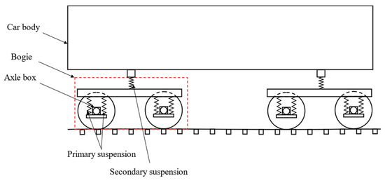
Figure 2.
Schematic of rail vehicle suspension.
The suspension system acts as a filter for the original waveform of the track geometry, thereby aggravating the nonlinearity between the track geometry and bogie vibration or track geometry and car-body vibration. However, sensors installed in the axle boxes are operated under sub-optimal working conditions, and thus, their timely maintenance is a challenging task. Therefore, researchers prefer to utilize the vibration data of bogies and car bodies for studying the characteristics [21]. Another type of mechanism-based method has been proposed, based on the theory of vehicle–track dynamics implemented via simulation models [22,23,24,25] in which the vehicle–track system is represented as a coupled system [21]. However, owing to heterogeneous influencing factors, such as the track structure, wheel–rail contact condition, and nonlinear suspension, the vehicle–track relationship features complex nonlinearities. Therefore, the mechanism-based method is unable to consider the various influencing factors with relative ease comprehensively [16], and the accuracy depends on the authenticity and reliability of the mode of system-parameter selection [26].
The signal analysis-based method directly analyzes the vibration signals [27,28,29]. However, this method is essentially linear processing of vibration data, and the running speed is generally assumed constant during processing [26]. In addition, considering that different TGDs have different features in the vibration signal after passing through the vehicle, determining the most feasible and effective feature types for each type of TGD is a challenging task [16].
2.2. ML-Based Train Vibration Data Analysis Method
In recent years, ML-based methods, represented by neural networks, have been widely used in rail transit infrastructure industries. It is challenging to extract TGD using CVD only [23]. However, with the development of ML models, certain valuable achievements have been made in this field [14,15,21,30]. Methods using solely ML models as classifiers, which is essentially an extension of the signal analysis-based method, still encounter the same difficulties in establishing defect features. Although black-box methods utilize models featuring strong nonlinear representation ability, the selection of the model architecture still requires further research. Existing models mainly employ the trial method, and thus, this approach hinders the ability to obtain the optimal model effectively.
2.3. Network Architecture Search in the Field of ML
Designing an ML model suitable for specific application scenarios requires expertise, extensive knowledge in the professional field, and considerable time to experiment [31]. In particular, the architecture is defined as the components constituting the model and its hyperparameters [32,33]. To optimize the model’s architectural performance effectively, researchers have proposed the network architecture search (NAS) theory [34]. This search strategy determines a model architecture offering the best performance using the search strategy based on the model’s performance-evaluation index () in a network architecture search space () [35]. Assuming that represents the dataset used for model training, represents a certain architecture of the model, and represents the weights in the model, the general form of NAS is expressed in Equations (1) and (2):
where and represent the randomly separated validation and training datasets obtained via , respectively. Common search strategies used in NAS problems include evolutionary algorithms (EA) [35], reinforcement learning (RL) [36,37], and gradient optimization (GO) [32]. Although EA-based and RL-based NAS methods can reduce manual intervention and obtain better-performing model architectures, these methods require computational resources that typically run on thousands of graphical processing unit (GPU) days [34]. To solve these problems, the GO-based NAS method, represented by DARTS [38], has gradually emerged as a solution. DARTS utilizes a relaxation method to transform the search space from discrete to continuous and uses a gradient-based method for optimization, and eliminates the need for extra components such as Controller [36] or Hypernet [39], thereby reducing the modeling difficulty and improving the optimization efficiency.
2.4. Discussion of Existing Research
In the problem encountered for TGD identification through portable-device-acquired CVD, existing research has mainly focused on signal analysis-based methods or ML-based methods to analyze the CVD. Although ML-based methods have demonstrated their potential for analyzing complex nonlinear relationships and the preliminary feasibility has been verified via simulation data, improving the identification accuracy is hindered in actual scenarios owing to certain obstacles. However, these ML models primarily perform architectural searches via the black-box trial method, which requires considerable time while offering a relatively low model performance. The TGD dataset represents a typical class-imbalanced dataset [40], resulting from a few instances of TGDs in a metro line. Therefore, a coping strategy is required to construct an ML model for TGD identification. In addition, existing TGD-identification models mainly leverage general evaluation metrics such as accuracy, precision, recall, and the area under the receiver’s operating characteristic curve (AUC-ROC). However, for the direct application of these metrics, the actual management needs of metro companies are not taken into account.
3. Problem Description
3.1. Basic Problem
The basic problem highlighted in this study was the CVD-based metro-TGD identification problem, in which the CVD was acquired using a portable detector. This problem was addressed by utilizing the CVD to determine the presence of a TGD on the metro track and to ascertain its severity level.
(1) The CVD was acquired using a portable detector on an ordinary in-service metro train in this study, and the data signal included the longitudinal, lateral, and vertical acceleration and angular rate of the car body, which conformed to the right-handed coordinate system (as illustrated in Figure 3A). The data obtained simultaneously also included speed, mileage, and location information. To minimize the additional influence of vehicle conditions on the CVD, the detector should be installed above the running gear, as depicted in Figure 3B. The portable detector [14] used in this study was developed by the State Key Lab of Rail Traffic Control and Safety at Beijing Jiaotong University. The size of the detector host is 270 mm × 170 mm × 91 mm, and its main components are illustrated in Figure 3C.
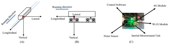
Figure 3.
(A) CVD coordinate system; (B) CVD acquisition location; (C) structure of the portable detector.
(2) A type of TGD, denoted . The severity level of this defect,, was classified into several levels according to the management regulations of the metro company, and the absence of defects was considered as a state of defect, , in this study.
3.2. Transformed Problem
The time-series signal-processing ability of CNNs is identical to that of recurrent neural networks (such as long short-term memory) but at a faster training speed [33], and these networks have been used to process vibration-signal data in several studies [32]. In this study, a metro TGD-identification CNN (MTGDI-CNN) based on DARTS is proposed to solve the CVD-based metro-TGD identification problem. Essentially, the basic problem is transformed into an MTGDI-CNN development problem. The research framework is shown in Figure 4. This study builds a metro TGD identification model based on a CNN, and uses the CVD and heterogeneity factors collected on in-service trains to construct samples suitable for the CNN model input. At the same time, it is assumed that the detection results obtained by the TGC are reliable, and the defect detection results are considered to be actual defects on the track. Thus, the samples are labeled with the TGC-defect reports collected on the same track at the same time as the CVD, to form the CVD-TGD dataset. Based on the dataset, the DARTS method is introduced to construct a MTGDI-CNN.
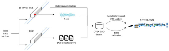
Figure 4.
Framework of this study.
The training process of a CNN model represents an optimization problem, as shown in Equations (3) and (4).
where denotes the sample, indicates the label and is its prediction, denotes the loss function, represents a CNN model, symbolizes the weights in the model, indicates the training dataset split from the original dataset , and denotes a dataset comprising samples and labels. Each pair in is termed an example, and is also named an example dataset. Further work is required to solve the MTGDI-CNN development problem.
(1) Design rules for CVD–TGD example dataset generation investigates the method of transforming the original data and prediction target in the CVD-based metro-TGD identification problem into input and output suitable for MTGDI-CNN. Moreover, it needs to consider 1) the method for transforming continuous CVD into discrete samples suitable for CNN input and 2) the heterogeneous factors between CVD and TGD that need to be introduced when generating the sample.
(2) MTGDI-CNN architecture design, training, and evaluation. The model architecture is designed according to the example dataset. CVD and TGD have a complex functional relationship that warrants an increase in the number of CNN layers to fit. However, adding layers to a CNN model with an ordinary simple architecture will lead to overfitting, thereby reducing the identification performance of the model [14]. Therefore, the NAS problem of MTGDI-CNN is a key problem to be addressed in the MTGDI-CNN development. This scheme must also consider (1) the reduction in the search space in Equations (1) and (2) the improvement of the training speed in Equations (2) and (3) the strategy to cope with the class-imbalance problem in the TGD dataset, and (4) the evaluation of the comprehensive performance of different model architectures in the context of the practical needs of metro management.
4. Metro Track Geometry Defect Identification Model and Its Optimization Method
4.1. Example Dataset Design
Each example in the dataset comprised a sample and label. The samples were generated using CVD, and the label was generated based on the same period as that reported by the TGC detection. The TGC detection report included the time, line information, and TGD records. The TGD record comprised the location, length, type, severity level, and other information concerning each defect.
4.1.1. Sample Generation Rules
Considering that the longitudinal acceleration is directly affected by the acceleration and deceleration of the train, this parameter was not included in the sample generation in this study, and only the remaining five vibration signals are considered—the lateral and vertical acceleration and the longitudinal, lateral, and vertical angular rates of the car body, denoted as , and the sampling frequency is denoted as . The CVD is highly correlated with the state of the track geometry variation [27], is significantly influenced by running speed [12], and is affected by the different vibration features under different vehicular conditions [41]. Therefore, the CVD (), running speed, and vehicle condition information were used to generate sample to account for the influence of these heterogeneous factors.
To fit the input of the CNN model, a continuous must be segmented. The actual metro-line mileage length of a data segment is denoted as , and the data segment is denoted as . Because is equal-time-interval (ETI) data with frequency,, the data count of varies, and the direct application of for sample generation results in different sample sizes, as indicated in Figure 5A. The reshaping technique, which depends on interpolation or downsampling, is a widely used strategy to address this situation in ML, such as difference-size image-processing tasks. Considering that equal-distance-interval (EDI) data (refer to Figure 5B) are usually leveraged in the field of track geometry detection, and the root mean square (RMS) value of the vibration signal is closely related to the track condition [15,42], an RMS-based [11] method is utilized to replace the reshaping technique in this study, which converts to EDI data such that features the same data count. The minimum data interval in the EDI data is , which is affected by the operating speed and the general length of TGDs, and this interval is usually 0.25 m [1].
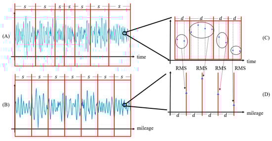
Figure 5.
(A) ETI data; (B) transformed EDI data; (C) zoom-in ETI data; (D) zoom-in transformed EDI data. (the RMS means root mean square).
As demonstrated in Figure 5C, let contain points in the minimum mileage data interval, , and the RMS value of th type of vibration signal of these points can be calculated using Equation (5).
where denotes the different types of vibration signals, represents the th point in mileage interval , symbolizes the value of the th point of th type of vibration signal, and indicates the RMS value of the th type of vibration signal. The converted EDI is denoted as , as indicated in Figure 5D. The data segment of within the mileage range, , is denoted as , where the point count is . is combined as an 5 matrix by mileage arranged form the smallest to largest, which is denoted as . Finally, generating the sample of the data segment with , average speed in the data segment and data-acquisition-train code, (), as expressed in Equation (6).
where =.
4.1.2. Sample Labeling Rules
In this study, the no-defect situation was considered as the state of defect, . When the metro TGD is divided into severity levels according to the metro company’s management regulations, states of the defect are present, corresponding to integers 0 to . In addition, the track segment within a mileage range of length was assumed to contain only one possible severity level corresponding to the defect. The assignment of label corresponding to sample data within a mileage range of length, , is represented in Equation (7).
4.2. MTGDI-CNN Based on DARTS
4.2.1. Model Architecture
The CVD is natural multi-channel one-dimensional (1D) data, and the signal amplitude of each channel fluctuates with the track mileage as a dimension. However, the specific type of TGD generally responds to the CVD of multiple channels [13,15,18,19]. Moreover, the vibration caused by the vehicle condition will be reflected in all CVD channels, and the intensity of these vibrations also varies with the operating speed [13,24]. Therefore, the metro TGD-identification model requires not only the ability to analyze various vibration data channels but also the ability to analyze the relationship between different channels. The most commonly used convolution operations in CNN are 1D convolution or two-dimensional (2D) convolution operations. One-dimensional convolution operation offers a more direct approach for processing the original vibration data for TGD identification without introducing other feature-extraction methods [43,44]. Several related studies have been conducted in the field of defect identification [32,45]. However, 1D convolution assumes that different channels of vibration data are relatively independent, and the ability to handle the relationship between different channels of vibration data is relatively weak. Considering the characteristics of CVD, the use of 1D convolution will reduce the TGD-identification performance. In this study, a 2D convolution was employed, and an MTGDI-CNN based on DARTS was proposed by collocating the vibration signals into 2D data, which realized the identification of metro TGD using a portable detector. The overall architecture of the model is illustrated in Figure 6.
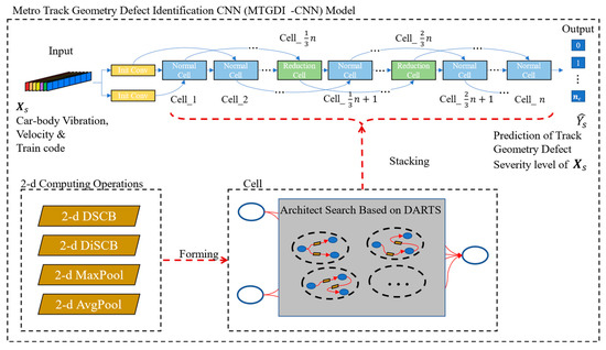
Figure 6.
Structure of MTGDI-CNN based on DARTS optimization method.
The main body of the MTGDI-CNN is composed of stacked cells, the input is sample generated from the CVD and heterogeneous factors, which are the speed and vehicle conditions, whereas the output is the predicted label of the severity level of defect within the mileage range, . The input is processed by the initial convolution (Init Conv) and subsequently processed by the stacking structure comprising the normal and reduction cells to output the predicted label, . Each cell in the stacked structure is connected to the previous two cells. The model contains two reduction cells located at 1/3 and 2/3 of the total number of cells. Each reduction cell is preceded by several normal cells.
4.2.2. Cell Architecture
Because directly searching for a space composed of connections between all operation layers is a challenging task, considering the presence of several identical architectures in neural networks, in the study of NAS, the entire network can be regarded as a stack of several cells with the same architecture, and only the cell architecture is targeted during the architecture search to mitigate the difficulty of the NAS problem [38]. The EA-based or RL-based methods, even in the face of the reduced search space of the cell architecture, still require a significant period of time. Accordingly, DARTS was employed in this study to search the cell architecture for solving the NAS problem in the MTGDI-CNN development.
The TGD is reflected as the amplitude variations of the CVD In an input sample. After processing via a feature extraction operation such as convolution, these variations are transformed into multiple sets of numerical vectors or matrices, which are called feature maps [46] and represent the vibration features of the TGD. As illustrated in Figure 7, a cell is a directed acyclic graph comprising several feature maps as nodes and feature extraction operations as edges [38]. Three fixed nodes and several intermediate nodes in each cell can be observed. Two of the fixed nodes serve as the input nodes, receiving the input of the previous cell, and a single node serves as the output. Each intermediate node is connected to the other two intermediate or input nodes, and all intermediate nodes are connected to the output node through concatenation. Additionally, the cells are classified into normal and reduced cells [47]. Moreover, the output feature map of the normal cell possesses the same size and channel number as those of the input. The output feature map of the reduction cell is half the size and twice the number of channels of the input. Such a cell architecture can not only extract the features of different lengths of TGDs but also deal with the relationship between different features.
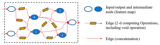
Figure 7.
Cell architecture (the number 0-3 means the order of the intermediate nodes).
4.2.3. Computing Operation Architecture
The 2D computing operations were employed as the cell edge to process the sample data for solving the CVD-based metro-TGD identification problem. The cell edge included a 2D depth separable convolution block (2D DSCB), 2D dilated separable convolution block (2D DiSCB), 2D max pooling (2D MaxPool), 2D average pooling (2D AvgPool), and void operation (only connecting without computing). Specific architectures of the 2D DSCB and 2D DiSCB are described in the following paragraphs.
The convolution-extracted feature is determined using the channel number of the convolution kernel. Therefore, the channel number of the kernel increases layerwise in a CNN model to fully extract the features. The kernel operates with all channels of the input feature map in an ordinary convolution. If ordinary convolution is used to process the CVD, the number of neural network computations will increase rapidly owing to the increase in the number of channels and cells, which leads to complexity in model training and a sub-par identification performance.
To mitigate this problem, several efficient neural networks have recently introduced operations such as deep separable convolution (DSC) [48] and dilation convolution (DiC) [49]. The DSC consists of two core elements: depthwise convolution and pointwise convolution. Depthwise convolution maintains a certain kernel width, but each kernel only processes one channel of the input feature map. The width of the pointwise convolution kernel is 1, and all channels of the input feature map are processed simultaneously. Using such a two-step convolution, a reduction in the computation number can be achieved while maintaining the feature extraction capability. The kernel of the DiC does not operate with the continuous adjacent elements of the input feature map but operates at a certain interval. For example, when the kernel width is three and the dilation parameter is one, the elements of the input data for the th operation with the DiC kernel change from to . The number of computations does not change, and the receptive field of the kernel expands. Such a DiC allows the kernel to cover a larger range of data by using the same number of computations, thereby improving the efficiency of feature extraction.
Therefore, to ensure accuracy and considerably reduce the computation number, 2D DSCB and 2D DiSCB were used to replace ordinary convolution when constructing the cells of MTGDI-CNN in this study. In addition to depthwise, pointwise, and dilation convolution, 2D DSCB and 2D DiSCB also include 2D batch normalization (2D BN) [50] and nonlinear rectified unit (ReLU) [51] to maintain the capability of independent feature extraction and replacement of arbitrary edges in a cell. The operations in a 2D DSCB or 2D DiSCB are arranged in the order of ReLU-Conv-BN [47,52], as illustrated in Figure 8. The kernel sizes in the 2D DSCB and 2D DiSCB can be set to different values to extract different sizes of TGD vibration features.
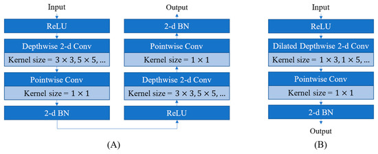
Figure 8.
Architecture of (A) 2D DSCB; (B) 2D DiSCB.
4.2.4. Cell Architecture Search Based on DARTS
Because of the aforementioned design, the cell has the ability to extract vibration features efficiently, but the connection mode of the feature maps (cell architecture) needs to be optimized according to the characteristics of the CVD-based metro-TGD identification problem. Cell architecture search (CAS) is a two-level optimization problem, as indicated in (1) and (2). In the problem, the cell needs several intermediate nodes and various computing operation kernel sizes to extract the vibration features of different-length TGD and analyze the relationship between the features. Therefore, the search space in (1) is still considerably large. However, the train-to-convergence process formulated in (2) requires considerable time. Therefore, the CAS persists as a difficult problem.
DARTS [38] was introduced to address this problem. To effectively search in the CAS search space, DARTS changed the space from discrete to continuous and used the gradient-descent method to improve the search speed. To reduce the time assumption of inner optimization, DARTS replaces the training-to-convergence process with a second-order approximation of the optimal weights based only on the first-generation training results. In a cell, the feature map of the intermediate node is calculated using Equation (8).
where denotes the computing operation that connects nodes and node . The traditional NAS search method involves searching for different combinations of discretely. In contrast, DARTS converts the fixed operation between nodes into a mixed operation , which is defined by a softmax value of all kinds of operations combined with weights , thereby changing the connection between nodes from discrete type selection to continuous weight change and realizing the transformation of discrete search space to the continuous variant, as demonstrated in Equation (9).
where denotes the mixed operations between node pairs , denotes the set of all alternative operations, and denotes the weight vector of the elements in . When the search is completed, the operation with the largest weight is utilized to replace the mixed operation, that is, the discrete cell architecture is restored, as expressed in Equation (10).
Let denote all architecture parameters in model architecture . The two-layer optimization model of Equations (1) and (2) can be expressed as Equations (11) and (12), respectively.
where denotes , and represents . Because (10) transforms the search space of the cell architecture into a continuous space, the gradient method can be employed for -optimization in Equation (12), that is, along the gradient to determine the minimum value iteratively. However, considerable time is required to train to converge; thus, DARTS only conducts one-generation training, utilizes its result to estimate the gradient to update , and assumes the updated as the approximate value of , as represented in Equation (13).
where denotes a small real number, termed the learning rate, and represents the approximate value of . The chain rule [53] is applied to further expand the gradient , as illustrated in Equation (14).
Because the second term of Equation (14) is a difficult parameter to calculate, DARTS employs the finite-difference approximation method to approximate it, as in Equation (15).
where denotes a sufficiently small real number, generally assumed to be , and .
4.2.5. Coping with Dataset Class-Imbalance Problem
Considering that the metro TGD represents an aberration and the limited number of physical instances of TGD in normal-operation metro tracks, the generated CVD–TGD example dataset, as detailed in Section 4.1, is a class-imbalance dataset. In general, the number of no-defect examples is considerably greater than that of level-II-defect examples [14]. The direct application of such a dataset for MTGDI-CNN training will lead to a detrimental effect [54], wherein the model will experience difficulties in learning features of a minority class of severity level, thereby reducing the effectiveness of the identification performance of this severity level. This problem is usually solved by weighting the model classification threshold or resampling the example dataset in the ML-based method. However, the threshold-weighting method must estimate the proportion of each class in advance; therefore, this approach is not applicable to CVD-based metro-TGD identification problem. The resampling method is classified into oversampling (OS) and undersampling (DS) methods. In particular, OS methods can be further classified as random OS (ROS) and synthetic minority oversampling techniques (SMOTE) [55]. SMOTE is a cluster-based synthesis method for minority class examples. Using the DS method results in several unlearned no-defect examples, and employing SMOTE yields several learned non-existing examples. Considering the high imbalance ratio and nonlinearity in CVD-based metro-TGD identification problem, the DS and SMOTE methods reduce the identification performance. Therefore, this study proposes the ROS method to address the class-imbalance problem in the MTGDI-CNN development, that is, to copy examples of a minority class of severity levels randomly.
Notably, the MTGDI-CNN was constructed in two stages: CAS and final model validation (FMV). To ensure that the model had sufficient generalization capability, a strategy using ROS only in the FMV training process was proposed. Considering that in CAS, the model architecture changes according to the features of the input example, the ROS method is not used in this stage to prevent excessive adaptation of the model architecture to the features of a minority class. In the FMV, the ROS method is employed to process the training dataset such that the model achieves improved training results.
4.3. Model-Performance Evaluation Metric
4.3.1. Selection Principles of Model-Performance Evaluation Metrics
Specific application scenarios must be considered when selecting the metrics for evaluating the model performance. When conducting TGD detection, metro companies are maximally concerned with the situation in which the actual TGD is not detected (missed detection) and the situation in which the detected TGD does not match the actual severity level (false alarm). Owing to the high requirement for the safety of metro operation, the situation of missed detections warrants more attention than that of false alarms. In addition, for the locations of false alarms, after high-frequency detection, they are relatively easy to confirm and eliminate.
4.3.2. TGD-Identification Performance-Evaluation Metric
The common evaluation metrics used in ML classification tasks are the precision and recall metrics. The higher the precision, the fewer will be the frequency of false alarms; the higher the recall, the fewer will be the frequency of missed detections. To account for the precision and recall, using their harmonic mean -score is a prerequisite [56], where represents the weighting factor of the recall, indicating the importance of the recall relative to the precision.
Considering the existence of different classes of severity levels, this study constructs a TGD F-score () (based on the -score of under each severity level of TGD), which is used to evaluate the comprehensive diagnosis performance of the model in the MTGDI-CNN development problem, as shown in Equations (16)–(19). is the harmonic average of the comprehensive prediction performance of the model for each severity level. The higher the value, the better the comprehensive identification performance of the model for each severity level of a defect.
where represents the class of severity levels of TGD, depicts the number of true positive cases (prediction class is , and true class is ) with class , symbolizes the number of false positive cases (prediction class is , and true class is not ) with class , represents the number of false negative cases (prediction class is not , and true class is ) with class , denotes the precision value of class , represents the recall value of class , and implies the -score value of class .
In addition, the occurrence of false positives (FP) and false negatives (FN) is often measured by the metrics false discovery rate (FDR) and false negative rate (FNR), as shown in Equations (20) and (21), respectively. Furthermore, there is a relationship between these metrics and precision and recall, as shown in Equations (22) and (23). Therefore, when is high, the proportion of FP and FN in the model will be low.
where denotes the false discovery rate value of class , and represents the false negative rate value of class .
5. Case Study
5.1. Case Data Description
The actual field dataset was acquired by the authors from 14 December 2020 to 16 December 2020, in Beijing Subway Line 1 captured via the portable detector, as described in Section 3.1. CVD acquisition was conducted for twelve iterations (eleven of them were complete runs, and one run lacked a metro section), six iterations for the down-direction track, and six iterations for the up-direction. Seven in-service trains were considered in the following order: 0, 0, 0, 1, 2, 2, 3, 4, 5, 6, and 2. The sampling frequency of the data was 250 Hz, and the data included the CVD, the train’s running speed, and mileage corresponding to the data. The TGD data were obtained from the TGC detection report dated 15 December 2020. In this study, LL defects (i.e., is LL) were selected to validate the proposed model, featuring 127 level-I LLs and 34 level-II LLs, and no level-III or level-IV LLs.
This study assumed the values of m and m to generate the example dataset. The sample size was (1-channel 2D data). A total of 16,659 examples were generated, including 15740 no-LL examples, 726 level-I-LL, and 193 level-II-LL examples. The example dataset only contained level-I and level-II cases, that is, the value range of the data label was .
5.2. Analysis of Identification Effect
To validate the generalization performance of the proposed model effectively, the original example dataset was segmented into the following four parts in this study: , , , and . The division method and proportions are indicated in Figure 9. was the same as the validating dataset reported by Wang et al. [14] and did not participate in the training and validation of CAS or in the training of FMV. Therefore, an objective evaluation of the generalization ability of the model was guaranteed.
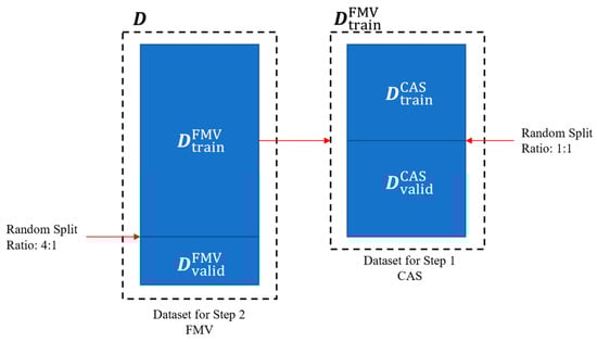
Figure 9.
Schematic of dataset division.
Simultaneously, to ensure the reproducibility of the case study, all random seeds were pre-assigned during the processes involving random number generation. The same divided datasets/sub-datasets were used for training and validating each model’s validation process.
5.2.1. Setting of Model Parameters
(1) Computing operations. According to the sample size, the kernel sizes were , , in 2D DSCB, , in 2D DiSCB, in 2D MaxPool, and 2D AvgPool. Featuring the void operation, eight elements were present in the alternative computing operation set of the cell edges.
(2) CAS. The number of stacked cells was eight, the channel number for the Init Conv was six, the batch size of each iteration was 128, and the number of training epochs was 50. The other parameters were in accordance with the DARTS basic setting [38]. Moreover, the number of intermediate nodes in the cells was four. The loss function was the cross-entropy loss function [53]. The inner optimization algorithm used was the stochastic gradient descent (SGD) [57], and the learning rate was updated via the non-restart cosine annealing method [58], with an initial value of 0.025, momentum of 0.9, and weight decay of 0.004. The outer optimization algorithm was Adam [59] with a learning rate of 0.004, momentum of , and a weight decay of 0.001.
(3) FMV. Different numbers of stacked cells and training epochs were set in this study to analyze the impact of these hyperparameters on the model performance, which is described in detail in later sub-sections. The number of channels for the Init Conv was six, and the batch size of each iteration was 512. The other parameters were in accordance with the DARTS basic settings [38]. The loss function employed was the cross-entropy loss function, and SGD was utilized as the optimization algorithm. To improve the training efficiency, cutout [60] and path dropout [61] with a probability of 0.2 were employed.
(4) Implementation and computing. The models in this case study were all implemented via the PyTorch [62] ML framework and were trained on a single NVIDIA GeForce GTX 1080 8 gigabyte GPU.
5.2.2. Model Identification Results
Based on the model settings detailed in Section 5.2.1, the CAS is carried out first in this section. According to the analysis in Section 4.2.5, the ROS method was not used to process the dataset in this stage, and the original datasets and were used directly; this was to limit the adaptation of the model architecture to features of minority class examples, which can reduce the ability to identify the general examples accurately. CAS was conducted using the computing resources and datasets mentioned above, and 50 generations of training required 0.3444 GPU days. The final cell architecture is shown in Figure 10.
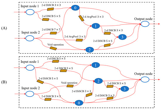
Figure 10.
(A) Normal cell architecture obtained from CAS; (B) reduction cell architecture obtained from CAS. (the transparent circles represent the input/output nodes, the normal circles represent the intermedia nodes, the arrows means the links between nodes and number 0-3 means the order of the intermedia nodes).
When cells are stacked to form the MTGDI-CNN, the model’s performance will be affected by different numbers of stacked cells and training epochs. Therefore, when performing FMV on the model constructed by the cell shown in Figure 10, this study set different numbers of stacked cells () and training epochs (epoch ) with a fixed random seed (0) for training and testing. A comparison of the and training time for different hyperparameter combinations is illustrated in Figure 11. For a convenient illustration, the model is denoted by , and all models with layers are denoted by .
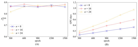
Figure 11.
(A) Comparison of for models with different hyperparameter combinations; (B) comparison of training time for models with different hyperparameter combinations.
As demonstrated by the results in Figure 11A, the performance growth of the models did not correlate optimally with the number of training epochs, indicating that the training of these models for 300 epochs was sufficient. The performance of the and models increased relatively with an increase in the training epoch, indicating that deeper models require more training epochs. When the model training converges, its comprehensive performance has a positive correlation with the number of stacked cells, and demonstrates a limited comprehensive performance improvement relative to ; however, the improvement effect of is not apparent compared with . As indicated in Figure 11B, the training time was proportional to the number of stacked cells and training epochs. The model with the superior performance was , featuring a value of 0.8838. The precision and recall of LLs at each level of are listed in Table 1. Evidently, after effective training, the model proposed in this study could use actual field data to identify LLs on the metro track and distinguish their severity levels.

Table 1.
Precision and recall of model.
5.3. Validation of the Effectiveness of Coping Strategies for Class-Imbalance Problem
5.3.1. Setting of Validation
Different dataset-processing modes were set in the two stages of CAS and FMV to form different coping strategies for the class-imbalance problem, and the model performance was compared based on the same test dataset to illustrate the effectiveness of the class-imbalance coping strategies proposed in this study.
The different coping strategies for the class-imbalance problem set in this section are shown in Table 2, where M-3 represents the strategy proposed in this study. “ROS” in the table indicates applying ROS to the dataset, and “ORI” indicates using the original dataset. Because the settings of BASE and M-3 in CAS are identical, these two modes of settings only conducted CAS once through the same cell architecture.
Table 2.
Dataset-processing mode settings for different strategies.
In addition, the metric sets a higher weight of recall, and different strategies have different results under different performance metrics. To avoid the bias caused by these different results in the analysis of effectiveness, two additional derived indicators, and , were calculated, in addition to calculating for various strategies in this study. is to replace in Equation (16) with ; thus, precision and recall are considered to have consistent weight when evaluating comprehensive performance. is to replace with ; thus, the weight of precision is considered to be one time higher than the weight of recall when evaluating comprehensive performance.
5.3.2. Results of Validation
To reduce the impact of different random seeds, three random seeds (0, 2, and 4) were utilized in CAS, and a fixed random seed was employed in FMV. First, three CAS modes were performed using three random seeds for each mode, and nine-cell architectures were obtained. The average training times for M-1/2/3(BASE) were 0.9289, 0.9363, and 0.3474 GPU days, respectively. The average training time varied for different modes because of the number of examples in the datasets, and the number of examples in was the main influence on the training time during the CAS, while the number of examples in exerted minimal influence.
Subsequently, a fixed random seed (0) was employed to retrain the model stacked by each cell architecture. Twelve combinations of the four modes and three random CAS seeds were trained and tested in the FMV stage, respectively. To conduct FMV with a lower time cost, the number of stack cells during FMV was set to eight, and the training epoch was 300. The average values of the performance metrics for different random seeds after training are listed in Table 3.
Table 3.
Model performance evaluation results.
Evidently, employing the ROS method on the FMV training dataset only significantly improved various performance metrics (comparing M-3 with BASE). In addition, the average training time was positively correlated with the number of examples used for training, and consequently, the average training time of M-1/2/3 remained unchanged, while the average training time of BASE was shorter. Among the performance metrics, the Avg. , Avg. , and Avg. increased by 8.0, 4.9, and 2.0%, respectively. This result implies that applying ROS to is a more effective strategy for improving comprehensive recall. Comparison of M-1, M-2, and M-3 revealed that the Avg. of M-3 was slightly lower than that of M-2, whereas the Avg. and Avg. metrics of M-3 were higher than those of M-1 and M-2, thereby demonstrating that M-3 could improve the comprehensive performance of the model, and it mainly improved the recall. Concurrently, the results indicate that the use of ROS in CAS will lead to insufficient generalization performance of the model architecture considering that the performance on the final validation dataset is average.
5.4. Comparison with Other Models
5.4.1. Comparison with the Model Constructed by 1D Convolution
To validate the 2D convolution scheme’s superior feasibility for the CVD-based metro-TGD identification problem, a 1D MTGDI-CNN (MTGDI-CNN-1D) was reconstructed and validated with the same division as that stated in the previous section. and were calculated simultaneously to avoid the bias of .
- (1)
- Setting of 1D model parameters
The 2D computing operations in MTGDI-CNN were replaced with 1D operations to form the MTGDI-CNN-1D. The sample size was reshaped from (one-channel 2D data) to (seven-channel 1D data) to fit the model input. The kernel sizes were 3, 5, 7, 11, and 15 in 1D DSCB, 3, 5, 7, and 11 in 1D DiSCB, and 3 in 1D MaxPool and 1D AvgPool. With the void operation, 13 elements were present in the alternative computing operation set of the cell edges. The other settings were identical to those described in the previous section. The experimental modes of the ROS are listed in Table 4.
Table 4.
Dataset processing mode settings for different strategies of 1D model.
- (2)
- Model validation results of 1D model
First, one experimental mode of CAS was performed (identical CAS settings were used for M-3-1D and BASE-1D), via three random seeds (similar to the methodology stated in the previous section), and three cell architectures were obtained. The average training time was 0.9584 GPU days. Subsequently, the fixed random seed, as stated in the previous section, was leveraged to retrain the model stacked by each cell architecture. Six combinations of the two modes and three random CAS seeds were trained. A comparison between the formulated performance metrics, based on the validating dataset and the values of M-3 stated in the previous section, is summarized in Table 5.
Table 5.
Model performance evaluation results of 1D model.
Evidently, the training time with the same example number in the FMV remained unchanged (upon comparing M-3 with M-3-1D), indicating that 1D convolution and 2D convolution offered considerable computational efficiency. M-3 of the 2D convolution exhibited the highest performance metrics; compared with M-3-1D, the three performance metrics for M-3 were 33.3, 30.0, and 26.8% higher, indicating that 2D convolution is more suitable for CVD-based metro-TGD identification problems. The comparison of M-3-1D and BASE-1D verified the conclusion stated in the previous section, that is, the coping strategy that only uses ROS for the training dataset in FMV could obtain a superior-performing model.
5.4.2. Comparison with the Model Obtained by a Black Box Trial Method
To verify the advantages of the MTGDI-CNN model based on the DARTS method proposed in this study compared with the model obtained by the ordinary black box method, this study compared the proposed model with the model obtained via the black-box enumeration method proposed by Wang et al. [14] (hereafter referred to as the Wang model).
The Wang model is built by constructing a functional layer (FL) with one ordinary 2D convolution operation, one ReLU, and one 2D MaxPool, and then simply combining multiple FLs and specifying the 2D convolution kernel size of different layers. The architecture of the Wang model can be determined by assigning four hyperparameters: FL layer number, the initial size of convolution kernel, minimum width, and the minimum height of the feature maps. Owing to certain limitations, only 360 models were available with different hyperparameter combinations, and Wang et al. [14] used the black-box enumeration method to search the architecture with superior performance. For comparison, the search space size was 8 ^ 14 in the proposed method.
Enumerated training and validation of the Wang models with 360 architectures were performed under three different random seeds, utilizing the same computational resources and dataset as mentioned in the previous section. The batch size of each iteration was 512, and the number of training epochs was 100. Under three random seeds, the process required an average of 2.1325 GPU days. In comparison, the proposed model (M-3) required an average time of 0.3474 GPU days, which was 83.6% lower. Subsequently, the average values of // of the 360 models under three random seeds were calculated. The maximum value of each average metric value was selected and compared with the results of the MTGDI-CNN (values of M-3 in Table 3), as summarized in Table 6. The performance of MTGDI-CNN was remarkably superior to that of the Wang models, and the three performance metrics were improved by 6.7, 2.7, and 0.1%. Thus, the proposed method can significantly improve the efficiency of the model architecture search compared with the common black-box enumeration method, and the MTGDI-CNN offers superior comprehensive performance.
Table 6.
Comparison of model performance evaluation results with those of black-box acquired model.
6. Conclusions
The proposed MTGDI-CNN enabled the effective integrated identification of the type and severity level of metro TGD via portable-device-acquired CVD on an ordinary in-service metro train.
The main contributions of this study were as follows: (1) The MTGDI-CNN based on DARTS was proposed, which realized the integrated identification of the type and severity level of metro TGD. The input of the model was the CVD acquired through a portable detector, and the output was the type of a TGD and its severity level. Compared to the traditional black-box trial method, by introducing DARTS into the problem scenario of this study, the efficiency and effectiveness of the model architecture optimization were considerably improved. (2) A strategy was proposed for coping with the class-imbalance problem of the dataset when modeling the MTGDI-CNN. This strategy reduced the impact of the low identification performance of the model through the use of the class-imbalanced dataset in the model architecture optimization and final training. (3) A metric was proposed for evaluating the comprehensive performance of the TGDs identification model. In the metric design process, the actual needs of metro track infrastructure management were considered, and this strategy was more conducive to improving the practicality of the model when used to evaluate its performance.
The following conclusions were drawn based on the results of the case study featuring actual data: (1) the introduction of the dataset ROS method in model development could improve the problem of poor model-identification performance caused by the natural class-imbalance characteristic of the CVD–TGD dataset. As for the two-stage optimization process of the MTGDI-CNN, the strategy of using the ROS method only in the training process in the second stage resulted in the overall improved performance of the model compared with other strategies that employ the ROS in other stages. Presumably, the model architecture had a stronger feature representation capability than the model weights, and therefore, overfitting was avoided in the architecture search stage, leading to a lower generalization capability, thereby yielding the aforementioned result. (2) The MTGDI-CNN could obtain higher comprehensive performance by increasing the number of stacked cells within a certain range; however, models with more cells required a longer period to train the same number of epochs, whereas models with more cells needed to train more epochs to converge. In this study, the case study revealed that after sufficient training, compared to 8-cell stacking, performing 16-cell stacking could result in a noticeable improvement in the model performance; however, performing 24-cell stacking did not yield a significant improvement compared to 16-cell stacking. The highest comprehensive performance represented by the value of 0.8838 was obtained for 16-cell stacking trained for 600 epochs in different combinations of the number of stacked cells and training epochs, with precisions of 0.9392 and 0.8528 for severity level-I LLs, and 0.6444 and 0.8529 for severity level-II LLs. (3) The DARTS-based modeling process could significantly reduce the optimization time of the cell architecture of the MTGDI-CNN and improve the final comprehensive performance of the model. The results of the case study showed that the optimization process using DARTS required 83.6% less time and improved the highest comprehensive performance () by 6.7% compared to a black-box acquired model under the conditions of using the same dataset and computing resources. (4) Two-dimensional convolution was more suitable than one-dimensional convolution for processing CVD to identify TGDs. The comprehensive performance () of the model built with 2D convolution was 33.3% higher than that of the model built with 1D convolution for identifying LLs. (5) could effectively evaluate the comprehensive performance of the model based on the field requirements of metro track infrastructure management. As indicated by the results of the case study, when evaluating different performance models, the model that satisfied the lower missed-detection case had a higher .
With the proposed method, metro track infrastructure managers can efficiently evaluate the metro track condition via portable detectors. At the same time, considering the similarity between metro tracks and railway tracks, the proposed method can be further extended to the detection of TGDs in conventional and high-speed railway tracks to improve the efficiency of infrastructure maintenance, but more data still need to be collected to verify the feasibility. However, this study had certain limitations. First, the proposed model was only used to validate and discuss the identification performance of the LLs of metro tracks at present. Second, this study assumed that only one TGD was present within a small distance (20 m in this study); thus, the proposed model needs to be further expanded for the special situation featuring multiple defects within 20 m. Finally, the actual data used in this study were limited in scope. To address these shortcomings, further research should focus on the applicability of other types of TGD. Additionally, sufficient data should be acquired to validate the model and further verify the model’s ability to handle actual situations.
Author Contributions
Conceptualization, Z.W. and R.L.; methodology, Z.W. and R.L.; software, Z.W.; validation, Y.G. and Y.T.; data curation, Z.W. and Y.G.; writing—original draft preparation, Z.W.; writing—review and editing, R.L., Y.G. and Y.T. All authors have read and agreed to the published version of the manuscript.
Funding
This research was funded by the National Natural Science Foundation of China (NSFC) under Grant 62132003, 71801010, and the Science and Technology Research and Development Plan Project of China State Railway Group Co., Ltd. under Grand (Temp-37).
Institutional Review Board Statement
Not applicable.
Informed Consent Statement
Not applicable.
Data Availability Statement
The dataset used in this study was available from a public data repository. The use of data follows the statement file in the repository: https://github.com/Elscip/scidata_jrrt_1. Access date: 30 March 2022.
Conflicts of Interest
The authors declare no conflict of interest.
References
- Soleimanmeigouni, I.; Ahmadi, A.; Kumar, U. Track geometry degradation and maintenance modelling: A review. Proc. Inst. Mech. Eng. Part F J. Rail Rapid Transit 2016, 232, 73–102. [Google Scholar] [CrossRef]
- Bai, L.; Liu, R.; Sun, Q.; Wang, F.; Wang, F. Classification-learning-based framework for predicting railway track irregularities. Proc. Inst. Mech. Eng. Part F J. Rail Rapid Transit 2016, 230, 598–610. [Google Scholar] [CrossRef]
- EN 13848-5:2017; Railway Applications—Track—Track Geometry Quality—Part 5: Geometry Quality Levels—Plain Line, Switches and Crossings. CEN (European Committee for Standardization): Brussels, Belgium, 2017.
- FRA (Federal Railroad Administration). Track and Rail and Infrastructure Integrity Compliance Manual: Volume II Track Safety Standards. 2018. Available online: https://railroads.dot.gov/elibrary/track-and-rail-and-infrastructure-integrity-compliance-manual-volume-ii-chapter-2-track-0 (accessed on 30 March 2022).
- GB/T 39559.4-2020; Specifications of Operational Monitoring of Urban Rail Transit Facilities—Part 4: Track and Earthworks. SAC (Standardization Administration of the P.R.C.): Beijing, China, 2020.
- Andrade, A.R.; Teixeira, P.F. Hierarchical Bayesian modelling of rail track geometry degradation. Proc. Inst. Mech. Eng. Part F J. Rail Rapid Transit 2013, 227, 364–375. [Google Scholar] [CrossRef]
- Xu, P.; Sun, Q.; Liu, R.; Souleyrette, R.R.; Wang, F. Optimizing the Alignment of Inspection Data from Track Geometry Cars. Comput.-Aided Civ. Infrastruct. Eng. 2015, 30, 19–35. [Google Scholar] [CrossRef]
- Zhang, Y.J.; Rusk, K.; Clouse, A.L. Decades of automated track inspection success and strategy for tomorrow. In Proceedings of the 2012 AREMA Annual Conference, Chicago, IL, USA, 16–19 September 2012. [Google Scholar]
- Sadeghi, J.M.; Askarinejad, H. Development of track condition assessment model based on visual inspection. Struct. Infrastruct. Eng. 2011, 7, 895–905. [Google Scholar] [CrossRef]
- Sadeghi, J.; Fathali, M.; Boloukian, N. Development of a new track geometry assessment technique incorporating rail cant factor. Proc. Inst. Mech. Eng. Part F J. Rail Rapid Transit 2008, 223, 255–263. [Google Scholar] [CrossRef]
- Jamieson, D.; Bloom, J.; Kelshaw, R. T-2000: A railroad track geometry inspection vehicle for the 21st century. In Proceedings of the 2001 AREMA Annual Conference, Chicago, IL, USA, 9–12 September 2001. [Google Scholar]
- Weston, P.; Roberts, C.; Yeo, G.; Stewart, E. Perspectives on railway track geometry condition monitoring from in-service railway vehicles. Veh. Syst. Dyn. 2015, 53, 1063–1091. [Google Scholar] [CrossRef]
- Balouchi, F.; Bevan, A.; Formston, R. Development of railway track condition monitoring from multi-train in-service vehicles. Veh. Syst. Dyn. 2021, 59, 1397–1417. [Google Scholar] [CrossRef]
- Wang, Z.; Liu, R.; Wang, F.; Tang, Y. Development of metro track geometry fault diagnosis convolutional neural network model based on car-body vibration data. Proc. Inst. Mech. Eng. Part F J. Rail Rapid Transit 2022, 236, 1135–1144. [Google Scholar] [CrossRef]
- Tsunashima, H. Condition Monitoring of Railway Tracks from Car-Body Vibration Using a Machine Learning Technique. Appl. Sci. 2019, 9, 2734. [Google Scholar] [CrossRef]
- Li, C.; Luo, S.; Cole, C.; Spiryagin, M. An overview: Modern techniques for railway vehicle on-board health monitoring systems. Veh. Syst. Dyn. 2017, 55, 1045–1070. [Google Scholar] [CrossRef]
- Scott, G.; Chillingworth, E.; Dick, M. Development of an Unattended Track Geometry Measurement System. In Proceedings of the 2010 Joint Rail Conference, Urbana, IL, USA, 27–29 April 2010. [Google Scholar]
- Weston, P.F.; Ling, C.S.; Goodman, C.J.; Roberts, C.; Li, P.; Goodall, R.M. Monitoring lateral track irregularity from in-service railway vehicles. Proc. Inst. Mech. Eng. Part F J. Rail Rapid Transit 2007, 221, 89–100. [Google Scholar] [CrossRef]
- Weston, P.F.; Ling, C.S.; Roberts, C.; Goodman, C.J.; Li, P.; Goodall, R.M. Monitoring vertical track irregularity from in-service railway vehicles. Proc. Inst. Mech. Eng. Part F J. Rail Rapid Transit 2007, 221, 75–88. [Google Scholar] [CrossRef]
- Wei, X.; Liu, F.; Jia, L. Urban rail track condition monitoring based on in-service vehicle acceleration measurements. Measurement 2016, 80, 217–228. [Google Scholar] [CrossRef]
- Li, C.; He, Q.; Wang, P. Estimation of railway track longitudinal irregularity using vehicle response with information compression and Bayesian deep learning. Comput.-Aided Civ. Infrastruct. Eng. 2020, 37, 1260–1276. [Google Scholar] [CrossRef]
- Kawasaki, J.; Youcef-Toumi, K. Estimation of rail irregularities. In Proceedings of the 2002 American Control Conference (IEEE Cat. No.CH37301), Anchorage, AK, USA, 8–10 May 2002. [Google Scholar]
- Lee, J.S.; Choi, S.; Kim, S.; Park, C.; Kim, Y.G. A Mixed Filtering Approach for Track Condition Monitoring Using Accelerometers on the Axle Box and Bogie. IEEE Trans. Instrum. Meas. 2012, 61, 749–758. [Google Scholar] [CrossRef]
- Tsunashima, H.; Naganuma, Y.; Kobayashi, T. Track geometry estimation from car-body vibration. Veh. Syst. Dyn. 2014, 52, 207–219. [Google Scholar] [CrossRef]
- De Rosa, A.; Alfi, S.; Bruni, S. Estimation of lateral and cross alignment in a railway track based on vehicle dynamics measurements. Mech. Syst. Signal Proc. 2019, 116, 606–623. [Google Scholar] [CrossRef]
- Ma, S.; Gao, L.; Liu, X.; Lin, J. Deep Learning for Track Quality Evaluation of High-Speed Railway Based on Vehicle-Body Vibration Prediction. IEEE Access 2019, 7, 185099–185107. [Google Scholar] [CrossRef]
- Tsunashima, H.; Hirose, R. Condition monitoring of railway track from car-body vibration using time-frequency analysis. Veh. Syst. Dyn. 2022, 60, 1170–1187. [Google Scholar] [CrossRef]
- Xu, L.; Zhai, W. A novel model for determining the amplitude-wavelength limits of track irregularities accompanied by a reliability assessment in railway vehicle-track dynamics. Mech. Syst. Signal Proc. 2017, 86, 260–277. [Google Scholar] [CrossRef]
- Paixão, A.; Fortunato, E.; Calçada, R. Smartphone’s Sensing Capabilities for On-Board Railway Track Monitoring: Structural Performance and Geometrical Degradation Assessment. Adv. Civ. Eng. 2019, 2019, 1729153. [Google Scholar] [CrossRef]
- Liu, R.; Wang, F.; Wang, Z.; Wu, C.; He, H. Identification of Subway Track Irregularities Based on Detection Data of Portable Detector. Transp. Res. Rec. J. Transp. Res. Board 2022, 2676, 703–713. [Google Scholar] [CrossRef]
- Wang, R.; Jiang, H.; Li, X.; Liu, S. A reinforcement neural architecture search method for rolling bearing fault diagnosis. Measurement 2020, 154, 107417. [Google Scholar] [CrossRef]
- Jiao, J.; Zhao, M.; Lin, J.; Liang, K. A comprehensive review on convolutional neural network in machine fault diagnosis. Neurocomputing 2020, 417, 36–63. [Google Scholar] [CrossRef]
- Li, X.; Zheng, J.; Li, M.; Ma, W.; Hu, Y. One-shot neural architecture search for fault diagnosis using vibration signals. Expert Syst. Appl. 2022, 190, 116027. [Google Scholar] [CrossRef]
- Ren, P.; Xiao, Y.; Chang, X.; Huang, P.; Li, Z.; Chen, X.; Wang, X. A Comprehensive Survey of Neural Architecture Search. ACM Comput. Surv. 2022, 54, 1–34. [Google Scholar] [CrossRef]
- Elsken, T.; Metzen, J.H.; Hutter, F. Neural Architecture Search: A Survey. J. Mach. Learn. Res. 2019, 20, 1–21. [Google Scholar]
- Zoph, B.; Le, Q.V. Neural architecture search with reinforcement learning. arXiv 2017. [Google Scholar] [CrossRef]
- Baker, B.; Gupta, O.; Naik, N.; Raskar, R. Designing Neural Network Architectures using Reinforcement Learning. arXiv 2017. [Google Scholar] [CrossRef]
- Liu, H.; Simonyan, K.; Yang, Y. DARTS: Differentiable Architecture Search. In Proceedings of the Seventh International Conference on Learning Representations (ICLR 2019), New Orleans, LA, USA, 6–9 May 2019. [Google Scholar]
- Brock, A.; Lim, T.; Ritchie, J.M.; Weston, N. SMASH: One-Shot Model Architecture Search through HyperNetworks. arXiv 2017. [Google Scholar] [CrossRef]
- Buda, M.; Maki, A.; Mazurowski, M.A. A systematic study of the class imbalance problem in convolutional neural networks. Neural Netw. 2018, 106, 249–259. [Google Scholar] [CrossRef]
- Bai, L.; Liu, R.; Li, Q. Data-Driven Bias Correction and Defect Diagnosis Model for In-Service Vehicle Acceleration Measurements. Sensors 2020, 20, 872. [Google Scholar] [CrossRef] [PubMed]
- Vinberg, E.M.; Martin, M.; Firdaus, A.H.; Tang, Y.; Qazizadeh, A. Railway Applications of Condition Monitoring; Technical Report; KTH Royal Institute of Technology: Stockholm, Sweden, 2018. [Google Scholar]
- Abdeljaber, O.; Avci, O.; Kiranyaz, M.S.; Boashash, B.; Sodano, H.; Inman, D.J. 1-D CNNs for structural damage detection: Verification on a structural health monitoring benchmark data. Neurocomputing 2018, 275, 1308–1317. [Google Scholar] [CrossRef]
- Sony, S.; Gamage, S.; Sadhu, A.; Samarabandu, J. Multiclass Damage Identification in a Full-Scale Bridge Using Optimally Tuned One-Dimensional Convolutional Neural Network. J. Comput. Civil. Eng. 2022, 36, 4021035. [Google Scholar] [CrossRef]
- Zhang, Y.; Xie, X.; Li, H.; Zhou, B.; Wang, Q.; Shahrour, I. Subway tunnel damage detection based on in-service train dynamic response, variational mode decomposition, convolutional neural networks and long short-term memory. Autom. Constr. 2022, 139, 104293. [Google Scholar] [CrossRef]
- Lecun, Y.; Bottou, L.; Bengio, Y.; Haffner, P. Gradient-based learning applied to document recognition. Proc. IEEE 1998, 86, 2278–2324. [Google Scholar] [CrossRef]
- Zoph, B.; Vasudevan, V.; Shlens, J.; Le, Q.V. Learning Transferable Architectures for Scalable Image Recognition. In Proceedings of the IEEE Conference on Computer Vision and Pattern Recognition (CVPR), Salt Lake City, UT, USA, 18–22 June 2018. [Google Scholar]
- Chollet, F. Xception: Deep Learning with Depthwise Separable Convolutions. In Proceedings of the 30TH IEEE Conference on Computer Vision and Pattern Recognition (CVPR 2017), Honolulu, HI, USA, 21–26 July 2016; pp. 1800–1807. [Google Scholar]
- Yu, F.; Koltun, V. Multi-Scale Context Aggregation by Dilated Convolutions. arXiv 2016. [Google Scholar] [CrossRef]
- Ioffe, S.; Szegedy, C. Batch Normalization: Accelerating Deep Network Training by Reducing Internal Covariate Shift. In Proceedings of Machine Learning Research, Lille, France, 6–11 July 2015; pp. 448–456. [Google Scholar]
- Nair, V.; Hinton, G.E. Rectified Linear Units Improve Restricted Boltzmann Machines Vinod Nair. In Proceedings of the International Conference on International Conference on Machine Learning, Haifa, Israel, 21–24 June 2010. [Google Scholar]
- Liu, C.; Zoph, B.; Neumann, M.; Shlens, J.; Hua, W.; Li, L.J.; Fei-Fei, L.; Yuille, A.; Huang, J.; Murphy, K. Progressive Neural Architecture Search. In Proceedings of the European Conference on Computer Vision (ECCV), Munich, Germany, 8–14 September 2018. [Google Scholar]
- Goodfellow, I.; Bengio, Y.; Courville, A. Deep Learning; MIT Press: Cambridge, MA, USA, 2016. [Google Scholar]
- Japkowicz, N.; Stephen, S. The class imbalance problem: A systematic study. Intell. Data Anal. 2002, 6, 429–449. [Google Scholar] [CrossRef]
- Bowyer, K.W.; Chawla, N.V.; Hall, L.O.; Kegelmeyer, W.P. SMOTE: Synthetic Minority Over-sampling Technique. arXiv 2011. [Google Scholar] [CrossRef]
- Chinchor, N.; Sundheim, B.M. MUC-5 evaluation metrics. In Proceedings of the Fifth Message Understanding Conference (MUC-5), Baltimore, MA, USA, 25–27 August 1993. [Google Scholar]
- Ruder, S. An overview of gradient descent optimization algorithms. arXiv 2016. [Google Scholar] [CrossRef]
- Loshchilov, I.; Hutter, F. SGDR: Stochastic Gradient Descent with Warm Restarts. arXiv 2017. [Google Scholar] [CrossRef]
- Kingma, D.P.; Ba, J.L. Adam: A method for stochastic optimization. arXiv 2014. [Google Scholar] [CrossRef]
- Devries, T.; Taylor, G.W. Improved Regularization of Convolutional Neural Networks with Cutout. arXiv 2017. [Google Scholar] [CrossRef]
- Srivastava, N.; Hinton, G.; Krizhevsky, A.; Sutskever, I.; Salakhutdinov, R. Dropout: A Simple Way to Prevent Neural Networks from Overfitting. J. Mach. Learn. Res. 2014, 15, 1929–1958. [Google Scholar]
- Paszke, A.; Gross, S.; Massa, F.; Lerer, A.; Bradbury, J.; Chanan, G.; Killeen, T.; Lin, Z.; Gimelshein, N.; Antiga, L.; et al. PyTorch: An Imperative Style, High-Performance Deep Learning Library. In Advances in Neural Information Processing Systems 32; Wallach, H., Larochelle, H., Beygelzimer, A., Buc, F.D.T.A., Fox, E., Garnett, R., Eds.; Curran Associates, Inc.: Red Hook, NY, USA, 2019; pp. 8024–8035. [Google Scholar]
Disclaimer/Publisher’s Note: The statements, opinions and data contained in all publications are solely those of the individual author(s) and contributor(s) and not of MDPI and/or the editor(s). MDPI and/or the editor(s) disclaim responsibility for any injury to people or property resulting from any ideas, methods, instructions or products referred to in the content. |
© 2023 by the authors. Licensee MDPI, Basel, Switzerland. This article is an open access article distributed under the terms and conditions of the Creative Commons Attribution (CC BY) license (https://creativecommons.org/licenses/by/4.0/).