A Data Factor Study for Machine Learning on Heterogenous Edge Computing

Abstract

As plants and animals grow, there are many factors that influence the changes that will affect how plants grow and how botanical experts distinguish them. The use of the Internet of Things (IoT) for data collection is an important part of smart agriculture. Many related studies have shown that remote data management and cloud computing make it possible and practical to monitor the functionality of IoT devices. In automated agriculture, machine learning intelligence is more necessary to use to automatically determine whether the correlation between learning factors influences plant growth patterns. In this research experiment, the relevant data are automatically collected through a detection device, and data modeling and computation are performed in an edge computing environment. At the same time, the data model is transmitted via the communication protocol, and another node is available for verification of the modeling and calculation results. The experimental results show that the single-point data-trained model is able to accurately predict the growth trend of the plants. In the case of verification of the second measurement point at a different space, the data model must be trained with more than two layers in order to improve the training results and reduce errors.

1. Introduction

In response to rapidly developing IoT technology, automated data collection technology can reduce a volume of manually recorded tasks and workflows. In addition, because of the accurate data collection technology, for the current machine learning technology, it has comparable technical analytical accuracy. At the beginning of data analysis, manual selection of factors is required, in which identification and assessment of those chosen known factors are made as known results, and those calculations regarding the results of the identification are related to the initial plane. However, while data analysis can analyze unknown information through various changes in time series, independent factors can be compared with selected dependencies. Deep learning (DL) algorithms are one of the most promising approaches in multiomic data analysis due to their predictive performance and their ability to capture non-linear and hierarchical characteristics.

Historically, the main mechanism of cultivating technology has been to use farmers’ experience and expertise to make decisions and determine corps parameters and planting conditions, and it is relatively impossible to complete the inheritance of experience. Before the maturity of the Internet of Things, there have been no data tracking and management to understand plant growth characteristics. Farmers’ visual judgements are based on changes in sky color and time interval, rainfall estimates, the status of farm drainage and water storage, and the need for early harvesting. Modern technologies use quantitative data to evaluate and make production decisions, and the application of data analytics is based on learned parameters and expert judgement. This study uses sensors to automatically collect relevant data and intends to use data association analysis to explore, compare and to analyze the trained model of the degree of correlation between each value. Based on our studies, the edge computing features would be used to establish observation points for factor index and plant growth conditions.

Currently, to understand the technical difficulties of collecting data, many studies have started to focus on signal data retrieved from IoT as the last-mile data-collecting method. Akhter, R. (2022) [1] studied the use of IoT data analysis applied machines to understand that the agricultural sector would have new crops to improve the quantity and quality of agricultural land production to meet the increasing food demand. Anik, S. [2] designed and manufactured a portable indoor environment data acquisition system named the Building Data Lite (BDL) model. Currently, in order to understand the technical challenges of data acquisition, some researchers have implemented new methods to extract signal data from IoT devices. For example, Akhter, R. (2022) [1] revealed the use of IoT data analysis applied machines to understand that the agricultural sector will have new harvests to improve the quantity and quality of farmland production to meet the increasing demand for food. Anik, S. [2] designed and manufactured a portable model of an indoor environment data collection system; in this study, they collected data from sensors such as temperature, humidity, light, action motion, sound, vibration and various gas sensors, in which the data collection mechanism can automatically obtain and manage the monitoring values of the controlled environment. In these research studies, it can be observed that automatically collecting data is useful for intelligent farm management and for analyzing more stable traces of growing data of agricultural plants.

1.1. Problem Definition

When it comes to data collection and modeling, edge computing data modeling environments tend to focus on edge data collection and model testing. Many studies have also started to explore the relevant technical descriptions of data hiding in data collection to improve the quality of service [3,4]. Various technical methods of data masking have been proposed to make the training set accurate and to take into account data-hiding events [5].

However, current hardware device design is mature, and the edge core processor is sufficient for limited project calculation and analysis. It is possible to compute and process data events directly on the edge equipment and to carry out computation and analysis through the edge equipment. The technical dilemma of having to hide data has been improved. In this research, we also consider the reduction of the system performance cost of computation. We store the sensed data in the edge device and perform computation independently through the device to improve the cost performance of the processor and memory access and computation writing.

From the study of Chan, Y.W. (2022) [6], through the successful resource management analysis technology in this study, both docker and grafana are guaranteed to have good performance results in terms of edge computing demands. Therefore, many researchers have started to discuss edge computing framework design, cloud and fog integration design, and other edge computing and cloud computing architectures [7,8]. The special feature of edge computing is that it is applicable to computing at the terminal nodes, which has many advantages.

A recent study by Kristiani, E. (2022) [9] found that computer vision accuracy can be improved by combining image data acquisition, training and predictive results. The accuracy of computer vision can be greatly enhanced by combining the image of the classifier and by labeling with edge computing, which can improve the optimization of deep learning models. In reviewing the above analysis, this research will use Raspberry tart features as the edge device. To reduce the penalty of yield, we will not specifically construct a Docker in our search. Rather, we will use a Linux environment for data access and similar computing.

The purpose of this study is to establish an experimental environment for the improvement of Internet of Things technology for data learning and to determine whether the modeling results can satisfy another plant growth model verification. In the training model, we first built IoT sensing devices to detect the growth cycle of Chinese cabbage and interactively verified the leaf length through the relevant data signals of soil and images.

1.2. Related Discussion

Based on the current research, we found that most of the research studies are focused on further IoT control operations after collecting agricultural data, including water valve management, light source management, etc. J Muangprathub (2019) [10] proposed to adopt a control system of the node sensors to carry out data management in the field through smart phones and web applications. Combined with web applications and mobile applications, mobile phone software design operations are performed, data retrieved from sensors are collected, and subsequent human intervention operations are performed.

This method samples data through device endpoints, makes judgments based on human experience, and manages related hardware. In contrast, current deep learning technology can be trained to gain more human experience and judgment without considering relevant outcomes. For example, during the growth of plants, it determines whether the fixed time of sunshine or the non-fixed time of sunshine will affect the growth results of the plants. Empirical studies on similar problems have not been made so far. The main reason for this is that the growth cycle of plants takes a long time, and the longer the timeline, the more disturbances there will be. Therefore, taking Taiwan as an example, the sunshine hours in the months of July and August are relatively long, which may affect the harvest status of vegetables, which in turn will affect the market value of vegetables.

Laha, A (2022) [11] previously designed an IoT communication system for automated irrigation water valves, which uses the MQTT protocol for monitoring the current environmental status and transmitting operation messages. This study mainly deals with remote controlling and monitoring operations but does not discuss predicting data. This study explores the possibility of further establishing a repeatable predictive and verified growth factor model through the predictive analysis model after data retrieval, referring to the communication and broadcasting framework proposed by Laha, A (2022).

Several studies have investigated LoRa-based communication models for distributed data collection [12,13]. LoRa is characterized by low power consumption. It can be used to reduce the amount of data transmitted after repeated data sampling. However, in this technology, due to a large amount of data sampling, data are observed and analyzed based on the data transmitted through the communication environment, but when used for machine learning and modeling, we can replace the data transmission of a large number of edge computing. Therefore, in the study, the computational model is placed on the edge device, the association model of computational result is transmitted to other nodes for verification through the MQTT broker, and the verification result report is used to change the association rule.

Guillén, M. (2020) [14] also discussed an edge computing platform that uses deep learning to predict low temperatures in agriculture. According to the study, to enable deep learning inference and training, edge computing needs to be performed by GPUs with higher performance in the computing environment. This is due to the cost dilemma between edge nodes, high-performance core computing environments, and real-world construction sites. A better GPU environment requires a lot of power-hungry computing, and most agricultural environment fields cannot provide a more stable power environment. This study refers to the federated learning model based on edge computing. Tsai Y-H [15] once proposed to use the edge environment setting to calculate separately first, and after data collection, use the calculation and analysis results to transfer to the training and learning endpoints through the communication environment. In the study, the images have been under training, and finally, the correct analysis results have been extracted. Therefore, by decomposing and analyzing various sensor data, only single items are collected and analyzed, such as temperature and growth trend calculations, or temperature and humidity trend calculations, etc.; Collection of individual data, writing of detection data to the database and use of CPU idle time. Calculation by MQTT publisher, sending of calculation and analysis results and sending of rules to broker. Data collection and modeling learning related to node processing can be completed through Broker Interactive Check, Distributed Training and Learning. We built models and experiments based on our research, improved the way of training the model, and cross-validated the analysis results.

In this study, the images from edge devices were taken, and eventually, the correct analysis results were retrieved. In the research, this disassembly calculation and feature analysis will be used to disassemble various sensor data and only by individual calculations such as temperature and growth patterns. Single-event factor calculation results are gathered and analyzed to determine the correlation between them, for example, calculating temperature and moisture trends, etc. The procedures for the experiments are listed as follow:

• Collect data from edge device.
• Write the data received in the database and use the CPU inactivity time for the calculation.
• Send the calculation and analysis results by MQTT Publisher.

We then send the rules to the broker through interactive audit and decentralization nodes, such as training and apprenticeship models. The models were built on the basis of our research, the training method of the model was improved, and the results of the analysis were validated.

The structure of this thesis is as follows: Section 1 is a review of the research description and previous studies. Section 2 explains the materials and methods, including our research framework, data computation methods, and factor selection formulas. Section 3 explains the experimental test results, the training matrix data and the built model through the machine learning modeling results. In Section 4, we discuss the issues identified in Section 3. We illustrate the feedback from the studies discussed. Finally, in Section 5, we discuss the results of the empirical application of this study and the model of the experimental application of the service.

2. Materials and Methods

2.1. Research Exploration Framework

In this study, in combination with the Internet of Things environment, based on the sensing equipment to establish a data collection model, and using the relationship management of the timeline to collect the sensing data information in accordance with the timeline operation, and data collection in accordance with the characteristics of the ground disturbance data, we established a data monitoring model under the state of deep learning.

In order to establish predictive model results, deep learning techniques can be repeatedly trained through data domains with different factors. For example, Ayturan, Y. A. (2018) [16] used deep learning modeling to learn about pollution data in real air and further explored the data results for the prediction of possible future pollution.

Read, J. S. (2019) [17] also explored the lake water temperature prediction model in their study and calculated and predicted the possible freezing time water temperature based on lake size, water flow, and the difference between cold and heat caused by weather effects. Hussain, D. (2002) [18] conducted a hydrological analysis study using convolutional neural networks (1D-CNN) and extreme learning machines (ELM) to predict interflow computations. In the same technical exploration, Yu, X. (2020) [19] used this calculation to measure sea surface water temperature. It can be seen that the selection of deep learning modeling factors can be achieved through repeated testing and verification of partial data sampling by sensing devices in different fields and at the same time by training and verifying the model on deep learning data time. Data sampling models can be established for correct natural environment prediction.

In this research, deep learning technology is used in combination with the Internet of Things for interactive verification. We tried to model the detection data from different locations and apply them to another similar cultivating environment for monitoring purposes. This study prepared both indoor and outdoor plant growth experiments, which used the outdoor plant growth trends and models for formation and prediction and determined the results of plant growth models. The confirmation of the accuracy of the model forecast was conducted by a self-test, and we transferred and shared the model using MQTT broker. The test terminal was designed for interactive testing. We attempted to send the plant growth characteristic factor selection result to another node to test if it can match the prediction result of the same node.

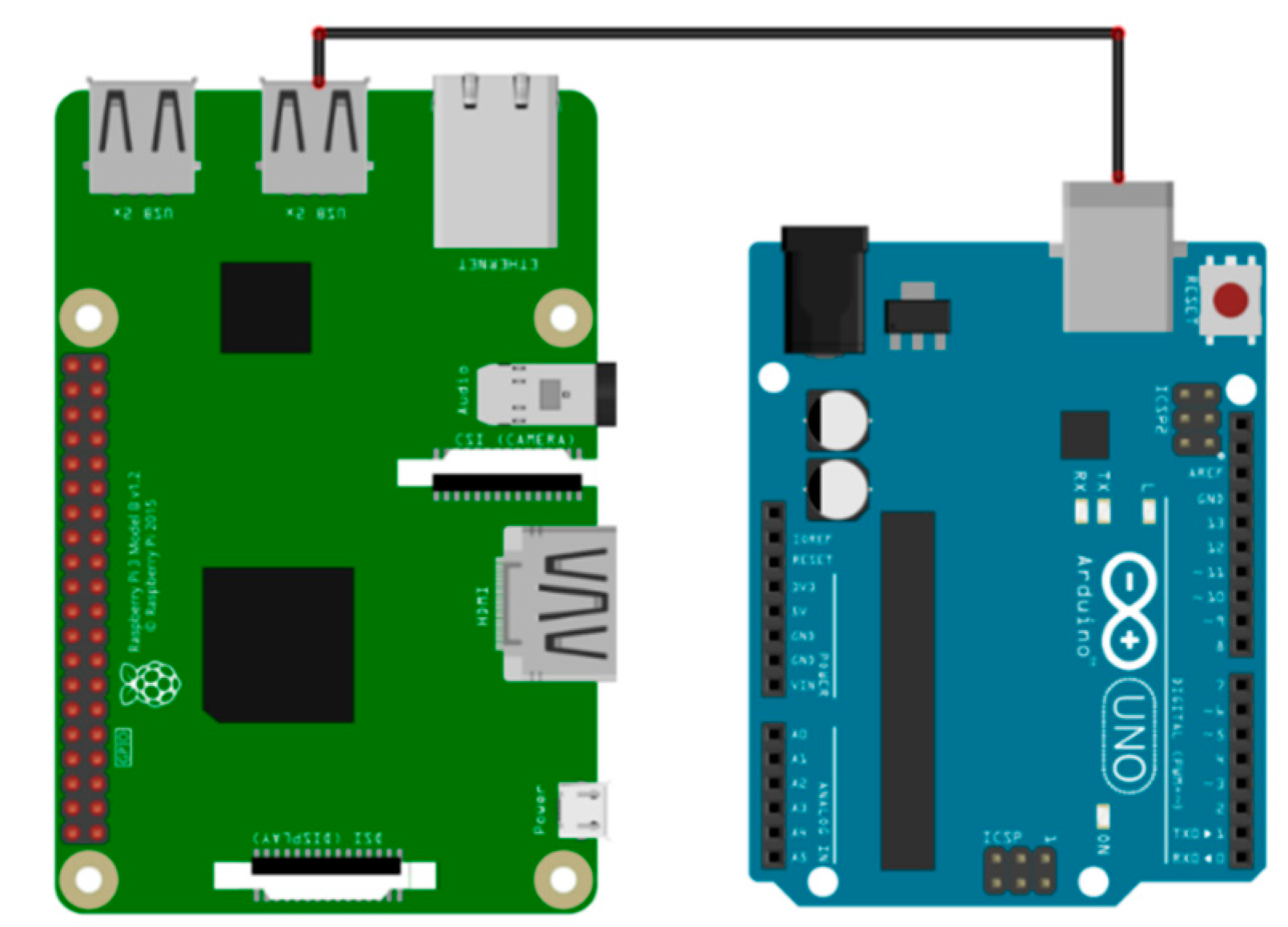
In order to make it easier to measure the detection data, we connected the Raspberry Pi to the Arduino unit through a USB connection, in which the detection data would be written to the Raspberry Pi for data processing and computation, as shown in Figure 1. The MQTT communication method was used for data analysis, which provides calculation results for prediction and verification to different nodes based on the calculation results of Raspberry Pi. In order to reduce the energy consumption and to obtain a better cycle of collecting and verifying the data during the searching process, we adjusted the wireless communication, which was sent to the Raspberry Pi, and a direct connection was used to write the data returned from the sensing device to the database. Finally, the data sampled in the database were computed and verified by Raspberry Pi, and the basic results were obtained by computing and analyzing the Long Short-Term Memory (LSTM) Recurrent Neural Network (RNN).

2.2. Data Collect and Analysis Architecture

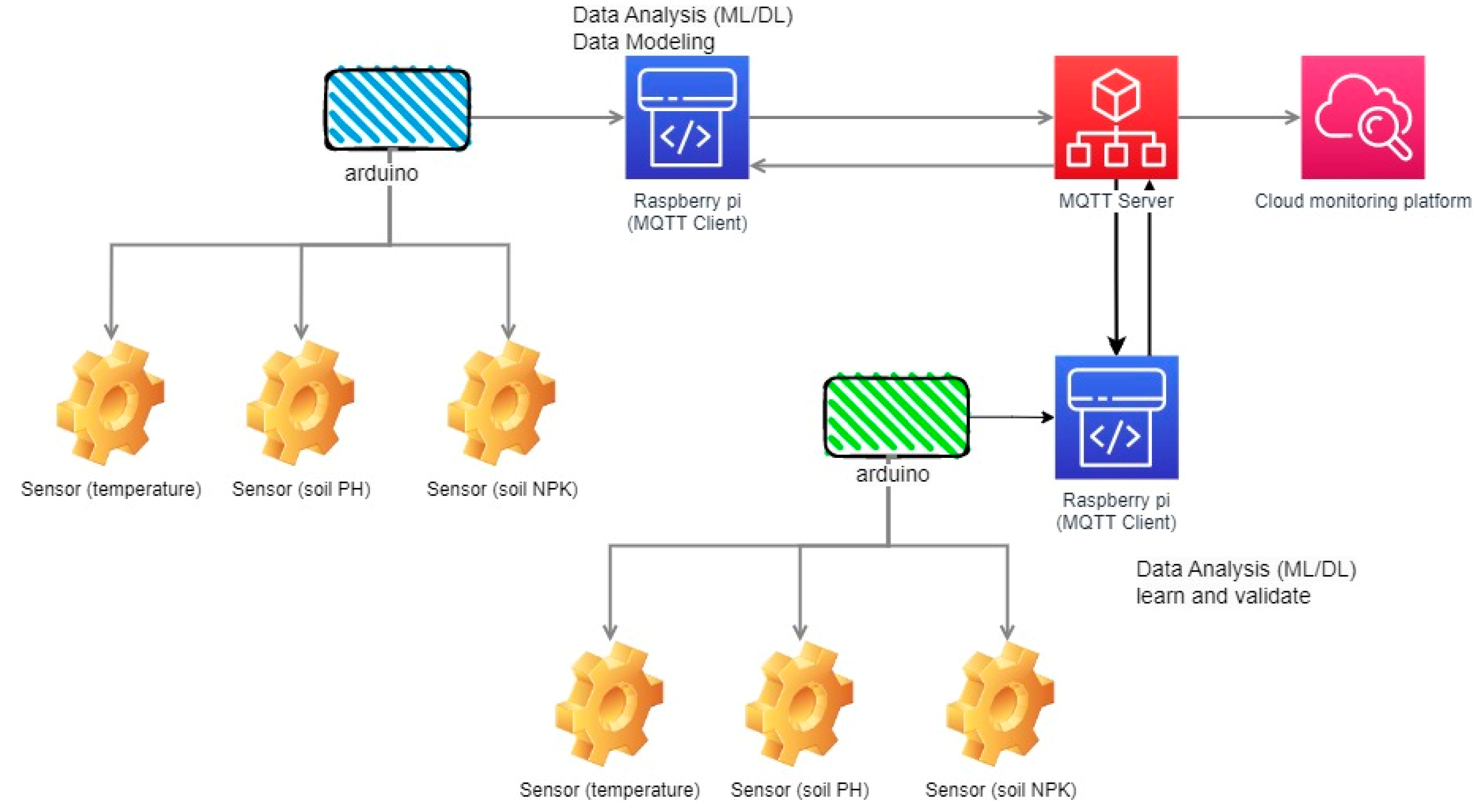
Taking the Arduino unit as the data collector, we conducted the measurements for 20 days by sampling data once per hour and by entering the constructed data for training into the database. The Long Short-Term Memory (LSTM) RNN model data training had been established, and the backhaul data based on time parameters had also been created. The Raspberry Pi creates data to shape the pattern. We set up five different tables for the calculation, including temperature, soil pH, nitrogen, phosphorous, potassium and leaf height. We used MQTT to apply the analysis model to another Raspberry Pi node, and the data model was sent to different experimental places and was used to verify the node status interactively, as shown in Figure 2.

Once the data are retrieved, we proceeded with a quantitative analysis of the data on the Raspberry Pi. The predictive growth trends had been established, and sophisticated depth learning models could be used to provide predictions of growth results. As the Chinese cabbage growing cycle is approximately 30 days, the value of the 20-day data is sufficient to shape and analyze the data, and the value of another node is used for prediction. In

Table 1. Data set collected from Arduino unit with Raspberry Pi.

	temp	ph	Nitrogen	Phosphorum	Potassium	Growth
0	18.0	5.8	54.0	8.2	73.0	0.000000
1	16.0	5.5	57.0	6.5	65.0	0.018780
2	17.0	5.0	42.0	4.1	57.0	0.033024
3	16.0	5.2	53.0	6.4	75.0	0.054930
4	17.0	5.4	57.0	8.0	84.0	0.065904
...	...	...	...	...	...	...
495	19.0	5.1	49.0	4.6	80.0	8.498526
496	20.0	5.1	53.0	6.8	79.0	9.645373
497	15.0	5.5	57.0	6.7	83.0	9.429895
498	19.0	5.0	45.0	5.0	65.0	10.655710
499	19.0	5.5	42.0	4.2	48.0	8.977325
500 rows × 6 columns

, we have extracted a part of the data.

The experiments were divided into three sections: training group, audit group and test group. In this study, the data are first collected and then validated. In parallel, training results are subject to model verification. We can see that the validated predictive formation model corresponds to the actual results. The test group then conducted post-test modeling forecasting experiments using control test groups at different locations. Prediction of the corresponding future growth rate and leaf length growth rate used preset factors such as temperature, soil pH, nitrogen, phosphorus and potassium.

2.3. Factor Calculation

With machine learning, it is possible that the models that build will fail to predict outcomes [20,21]; thus, a lot of work has been conducted on how to minimize the loss functions. In reality, the predicted value cannot be exactly the same as the real value. In principle, there will be a difference between the predicted value and the real value. Therefore, in machine learning, the mean square error can be used for computing and processing, and the expected mean absolute error can be obtained after correction. The obtained MSE can be squared plus the square root sign, and the error output can be corrected in the same units as the data. The value can be used for efficient training on prediction results and numerical verification. We also found that many studies have begun to use RMAE to calculate machine learning variables, such as soil acidity or foliar disease detection [22,23].

We evaluated the predictive power of the model by establishing the root mean square error (RMSE). The mean square error may be used to derive the regression loss function. The method of calculation is the sum of the squares of the distance between the forecast value and the true value.

$$RMSE=\sqrt{\frac{1}{N}{{\displaystyle \sum }}_{i=1}^N{\left(y_i-{\widehat{y}}_i\right)}^2}$$

(1)

We first read the data to generate the database’s expected analysis data form.

3. Results

In addition, the Arduino communication system is used as a data acquisition and communication system. Arduino is used to collect data from the sensor side and send information such as temperature, moisture, soil pH, etc., to the database of the Raspberry Pi device via a USB connection. Based on the collected data, Raspberry Pi builds a data learning model. In the modeling of data processing, the data are learned from different factors, and the system automatically compares them based on different vector factors and proposes appropriate suggestion results. For the MQTT participant, the Raspberry Pi machine will compare the collected data with the received data automatically. The simulation architecture of our experimental scenario is shown in Figure 3.

During data training and learning, we must select a communication protocol to verify the data training template. In our research, we use MQTT’s communication protocol to establish a recording and communication mechanism. The MQTT communication protocol was made publicly available by QASIS in 2013. It provides a publishing-subscription transmission protocol and provides the status of the mutual transmission data in M2M/IoT mode.

In this study, the model was built after the data are fed to the remote server by MQTT on the Raspberry Pi node. Along with another set of Raspberry Pi, hardware is used to check the training results. The audit results are sent to the cloud platform synchronously so that users can use them and see if the changing curves of different vegetable growth factors in different environments show different results.

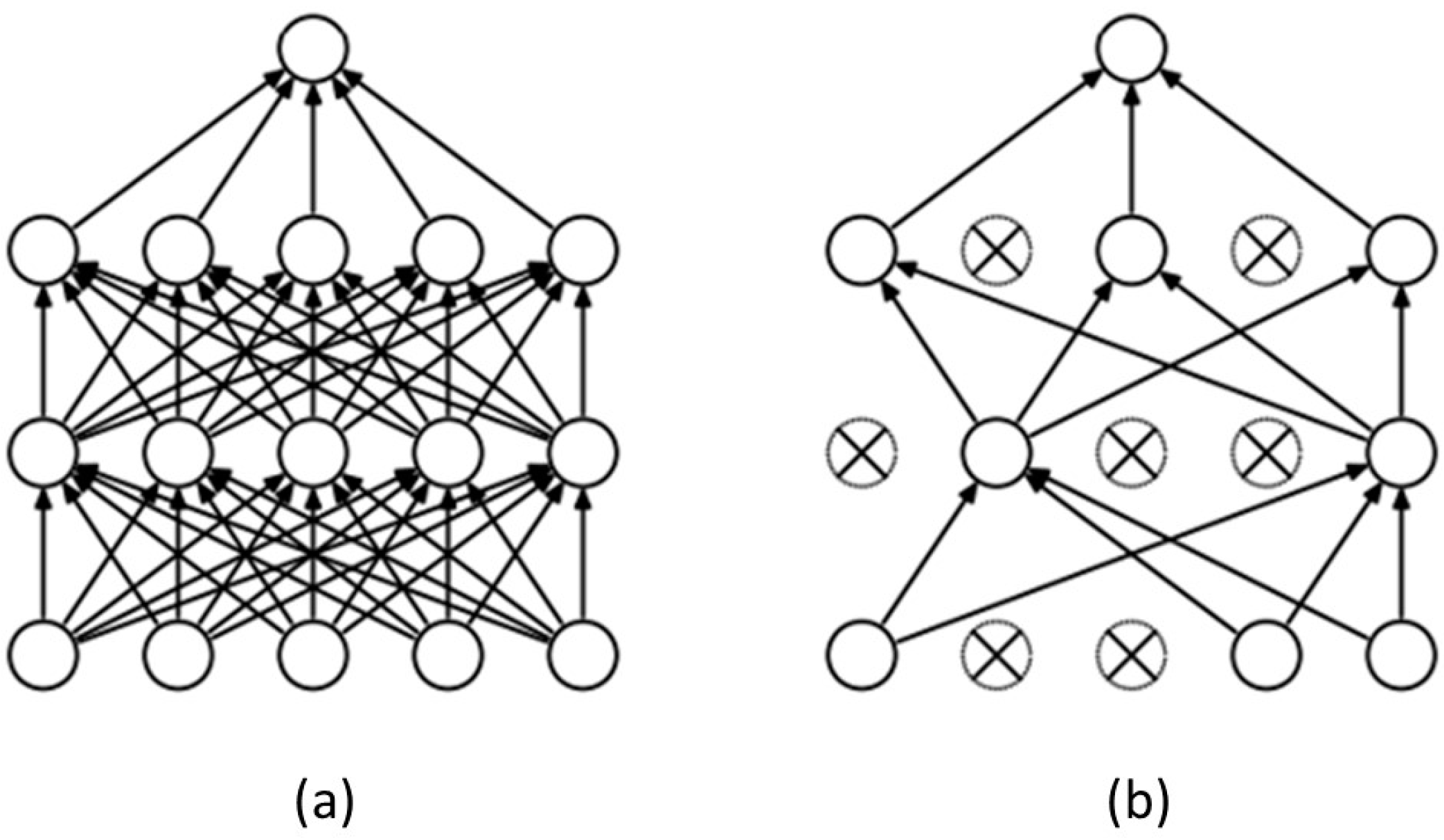
To make repetitive training results more accurate in a standard neural network, a probability representing the possibility of stopping each neuron is usually established in the exclusion layer. Its main goal is to stop that node and let another node conduct the computation (Figure 4).

Considering the data to avoid excessive simulation calculations and possible distortion in deep learning processing, the exclusion mechanism was added to construct each layer of the neural network and to fix the probability of elimination of the nodes in the neural network. Some content from each training course is extracted, giving the data back during the repeated workout and then extracting another portion of the data content to gradually increase the authenticity of its workout and to prevent overflow.

The model structure using dropout had been defined as listed in

Table 2. Setting dropout within d = 0.3.

def lstm_model0(input_length, input_dim):

d = 0.3

model = Sequential()

model.add(LSTM(32,input_shape = (input_length,input_dim),return_sequences = False))

model.add(Dropout(d))

model.add(Dense(1,activation = ‘linear’))

model.compile(loss = ‘mse’,optimizer = ‘adam’)

return model

.

Data Modeling

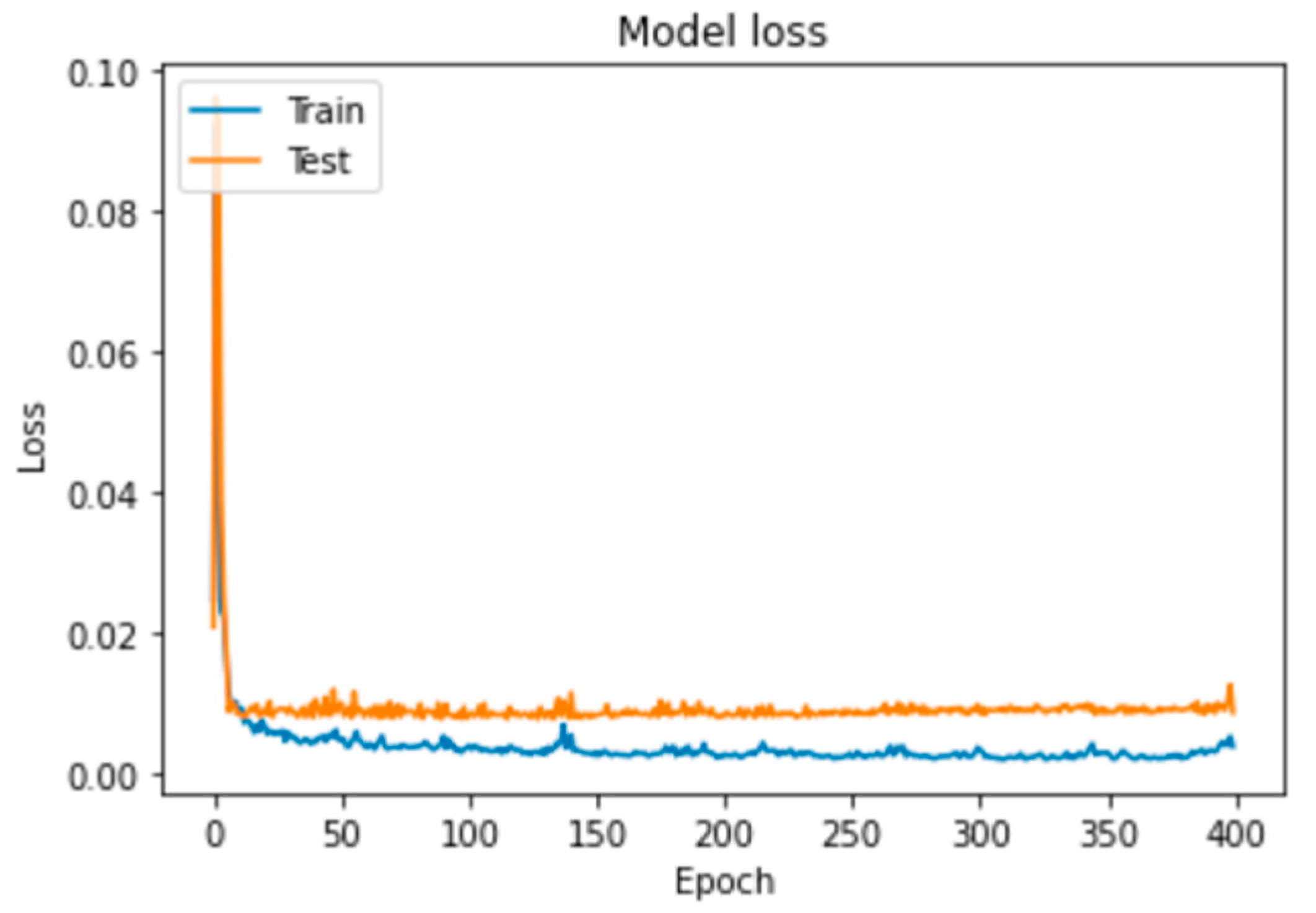
In the experiments, we initially formed the model based on the data collected. In the modeling approach, 30 sample data were taken each time for a total of 400 epochs. Only the models with better predicting results are acceptable. If this is not better than the outcome of the previous training, the outcome of the training is set aside.

The parts of output of the training processing are listed in

Table 3. The model is trained to access only the most specific outcomes.

Epoch 26/400

8/13 [=================>............]-ETA: 0s-loss: 0.0036

Epoch 26: val_loss did not improve from 0.00801

13/13 [==============================]-0s 11ms/step-loss: 0.0058-val_loss: 0.0090

Epoch 27/400

9/13 [===================>..........]-ETA: 0s-loss: 0.0049

Epoch 27: val_loss did not improve from 0.00801

13/13 [==============================]-0s 11ms/step-loss: 0.0058-val_loss: 0.0092

Epoch 28/400

8/13 [=================>............]-ETA: 0s-loss: 0.0034

Epoch 28: val_loss did not improve from 0.00801

13/13 [==============================]-0s 10ms/step-loss: 0.0061-val_loss: 0.0092

Epoch 29/400

9/13 [===================>..........]-ETA: 0s-loss: 0.0038

Epoch 29: val_loss did not improve from 0.00801

13/13 [==============================]-0s 9ms/step-loss: 0.0045-val_loss: 0.0090

. The numbers of trained parameters for different models, which were used on those experiments, are shown in

Table 4. Information was consolidated following the formation of the first layer.

Model: “sequential”
Layer (type)	Output Shape	Param #
lstm (LSTM)	(None, 32)	4992
dropout (Dropout)	(None, 32)	0
dense (Dense)	(None, 1)	33
Total params: 5025
Trainable params: 5025
Non-trainable params: 0

and

Table 5. Information following two training jobs.

Model: “sequential_1”
Layer (type)	Output Shape	Param #
lstm_1 (LSTM)	(None, 10, 128)	69,120
dropout_1 (Dropout)	(None, 10, 128)	0
lstm_2 (LSTM)	(None, 64)	49,408
dropout_2 (Dropout)	(None, 64)	0
dense_1 (Dense)	(None, 1)	65
Total params: 118,593
Trainable params: 118,593
Non-trainable params: 0

.

4. Discussion

Our experiments aim to learn and predict the growth data of two identical plants in different locations. The main reason for this is that the growth data are expected to be learned by planting outdoors. Once the model is established, it will be transferred via MQTT to another indoor planting location. Since the outdoor growth environment needs to be simulated indoors and the experimental parameters are set manually, in the future, more IoT devices can be combined to set the environmental conditions automatically and in the outdoor environment. Therefore, the outdoor growth model of this study is very important for the training of indoor plant growth trends. For this reason, in this study, we first modeled the results of outdoor training, and when the trained model was tested with the prediction results of plant growth in the same environment, the trained model and the prediction results agreed with the prediction results of plant growth in the same environment. However, if we change the test terminal and feed the model with indoor plant growth data to predict the next growth trend, we find that its accuracy in predicting growth decreases.

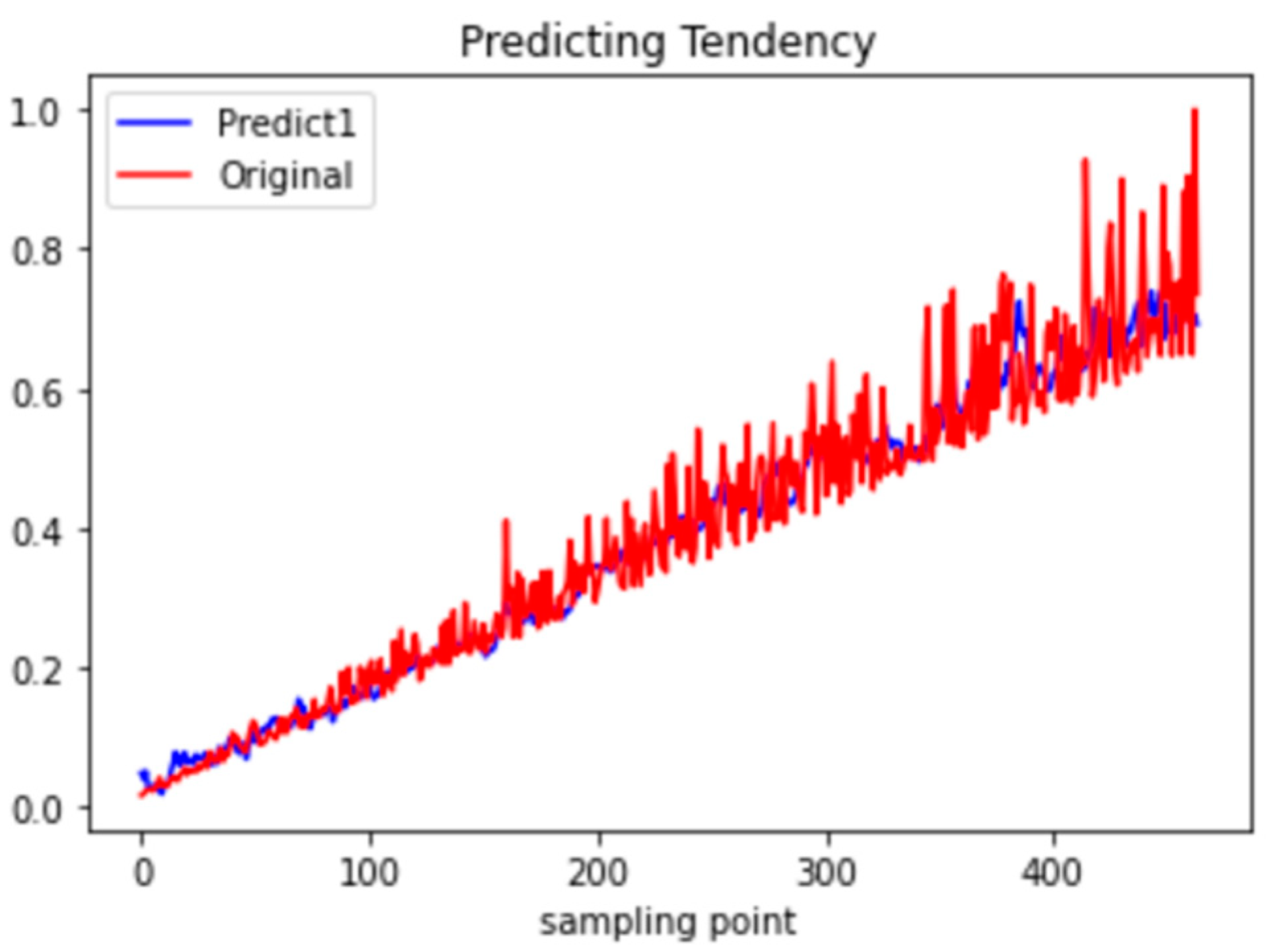
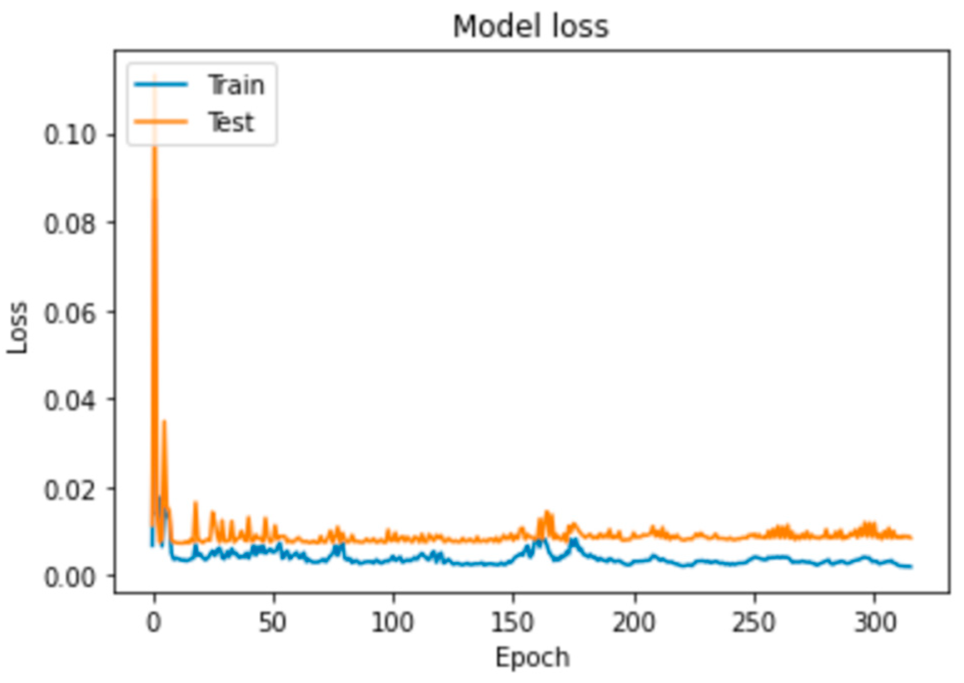
This section shows the parameter setting and discussion about the experimental results. Based on training data sets, we allowed the machine to perform 20 days of data training each time and learn the five factors that we collected at the same time. In the post-training results, as shown in Figure 5, Figure 6 and Figure 7, only the first layer serves for training and validation. The findings are presented in Figure 6, where predictive models vary greatly.

Retraining and learning on the same data set were performed in the experiments. The average difference was too large, even though the formation and prediction results of the same parent data were very accurate. While this may be due to the growth characteristics of the plant, the environment data may not have a direct correlation with the growth trend results. However, if the same data set is used, it is always possible to have an efficient prediction that the result is consistent with the original result. In the study, the predicted calculation results and actual data are shown in Figure 8, where the data set training result model was applied to the second non-homologous training test object. From comparing the linear difference, we can clearly see that there is a difference. Especially for the test data from 5 to 10, there is a significant difference in the linear results.

In Figure 7, the growth data of 25 experimental plants were randomly selected; the blue line represents the deep learning prediction, while the orange line represents the experimental data. In our study, we used the predicted size of the plant’s leaf growth as a benchmark. Most of the prediction models are able to predict that the average growth will be in the range of 8 to 10 mm. The training data set was calculated based on daily plant growth. Therefore, it includes temperature, pH, nitrogen, phosphorus, and potassium. We measured these according to the estimated growth rate. In this way, the same factors can occur but fall within different growth cycles, resulting in different growth values of the corresponding growing leaves. In the results of the prediction, we can observe more precisely that the difference in the prediction can be up to 2 mm. Previously, this discrepancy was not visible to the naked eye.

Therefore, in the research process, we adjusted and conducted as many secondary experiments as possible. We can consider that in a different growth information node, when there is a gap between its variation in growth and the result of the formation, the training model will perform another layer of improvement. In the case of the study, we observed that there was still a difference. The MSE was reduced from 7.8 to 0.09 when the training results were compared with the actual data. This means that the “deeper” the layer is in the model, the more the model’s prediction accuracy can improve.

Therefore, we can use the same data set for the second repetition of the training. The results of the training are shown in Figure 8. The findings show that the blue waveform has more vibrations after training. In comparison to Figure 5, the loss of the model has a higher accuracy after training and testing the same model. The experimental results were tested on the prediction results from the initial data, and it is still possible to see that the relevant values of plant growth are not fully compatible with the intended results. After the second training, the accuracy of the model was still good.

In the use of experimental training and testing of training results, it can be observed in the research that data from the data set can be validated by training on the data set itself. The experimental results shown in Figure 6 were highly efficient, which indicates that the construction of the predictive growth model succeeded. However, as shown by the results in Figure 8, when we apply the experimental results to the second edge design node, its computational prediction performance is significantly reduced. Figure 8 compares the expected trend adjustment of samples 5 to 10 with Figure 7, showing good correction performance due to repeated learning and modeling, reducing the expected bias rate and improving prediction accuracy. For this reason, the improvement of the accuracy of the experiment is an attempt to improve the accuracy of the training package data through two-stage learning, where we provided a second training on deep learning modeling. Show as Figure 9 and Figure 10.

5. Conclusions

In this study, we used a processor kernel in the Raspberry Pi environment based on an edge device to rebuild the IoT data collection and training model under advanced computing. In our experiments, we developed relevant data and results for leaf growth trend analysis using sensor data collection and simulation training. From the experiments, we can observe that in a single training model, the prediction results and the actual growth trend can be accurately predicted, but when the pattern of training is out of center, the prediction results and the actual growth trend can be out of center. However, when the pattern of training results is applied to another test node, the five relevant factors and the prediction results need to be further deep-structured to achieve more accurate predictions.

The current research on plant growth factors used only five elements selected for experiments; thus, the information on unobserved factors may be observed and discovered through experience, and other factors may be added in the future to improve forecast accuracy.

Edge computing is used to predict or calculate plant growth characteristics. The main purpose is to solve the problem of agricultural experts assessing and observing plant growth trends based on past experience. After global warming, environmental and climatic factors are more complex than before. Indoor planting has been popular in recent years, but the growth effect of plants is still limited. The main reason is that the past experience judgment is based on the agricultural experience of field planting, but after changing environmental information, it exceeds the experts’ past experience judgment results. Therefore, we have started to collect and monitor plant growth factors in our research and to predict trends that may affect plant growth according to different factors.

In this study, the training pattern is assigned to different nodes for experiments by combining IoT and machine learning modeling with the concept of cloud fog fusion. In the future, this search template can be used to perform more verification on many different edge nodes; thus, improving the accuracy of analytical data and predictive information could be enhanced.

Our research is limited to the corresponding analysis of the five proposed factors on plant leaf growth size, first verifying whether different factors can predict plant growth trends and the accuracy of growth prediction data. In the research, we took out five factors including temperature, soil pH, soil nitrogen, soil phosphorus and soil potassium and calculated them according to the growing length of the leaves. As there may be other factors such as air pollution, hours of sunlight, average air temperature and so on, these other variables may be used in future studies to add numeric information to the automatically collected and computed elements.