
Interference Suppression in EEG Dipole Source Localization through Reduced-Rank Beamforming


Abstract
1. Introduction
2. Materials and Methods
2.1. Data Model
2.2. Beamforming and Neural Indices
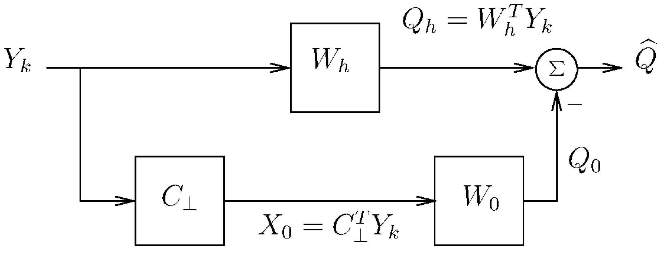
2.3. Generalized Sidelobe Canceler
2.4. Adaptive Blocking Matrix
2.5. Proposed Reduced-Rank Beamforming Scheme
2.6. EEG Data
2.6.1. Simulated Data
- signal-to-measurement-noise ratio, given bywhere denotes the Frobenius norm;
- signal-to-biological-noise ratio, given by
2.6.2. Real EEG Data
3. Results
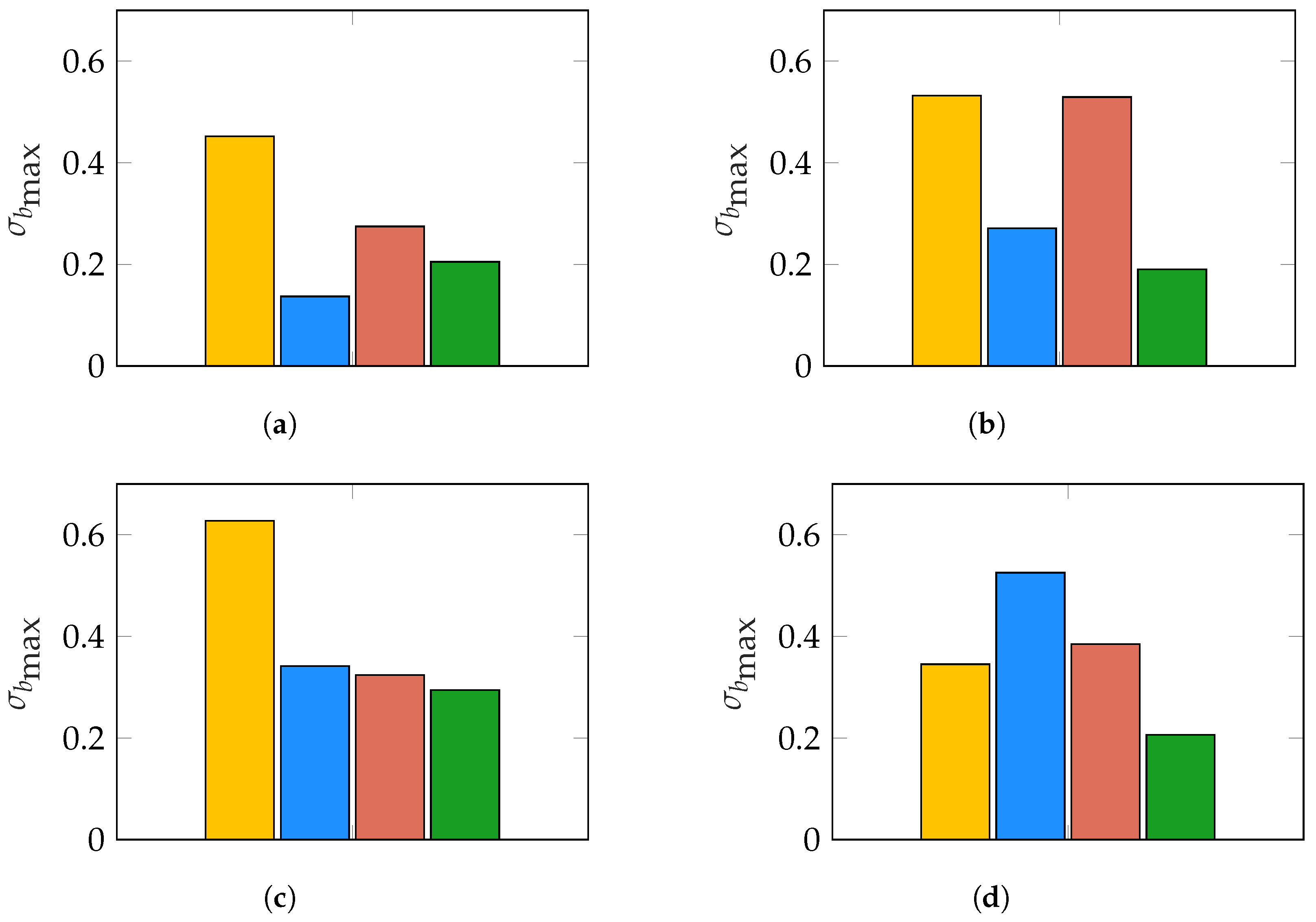
3.1. Evaluation of Performance under Different and Conditions
- the individual bias of the estimates, given by ;
- their sum-of-squares: ;
- the maximum bias: .
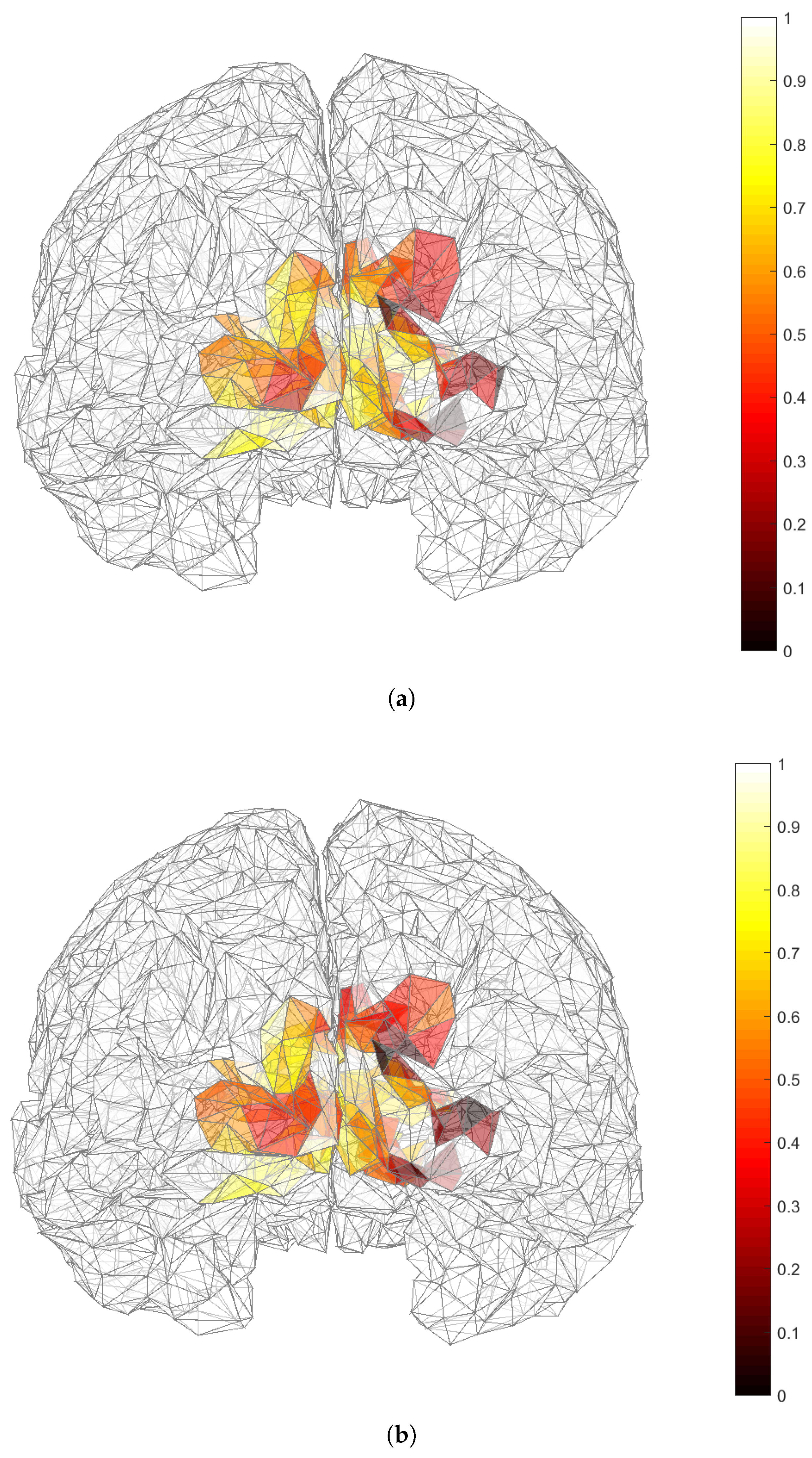
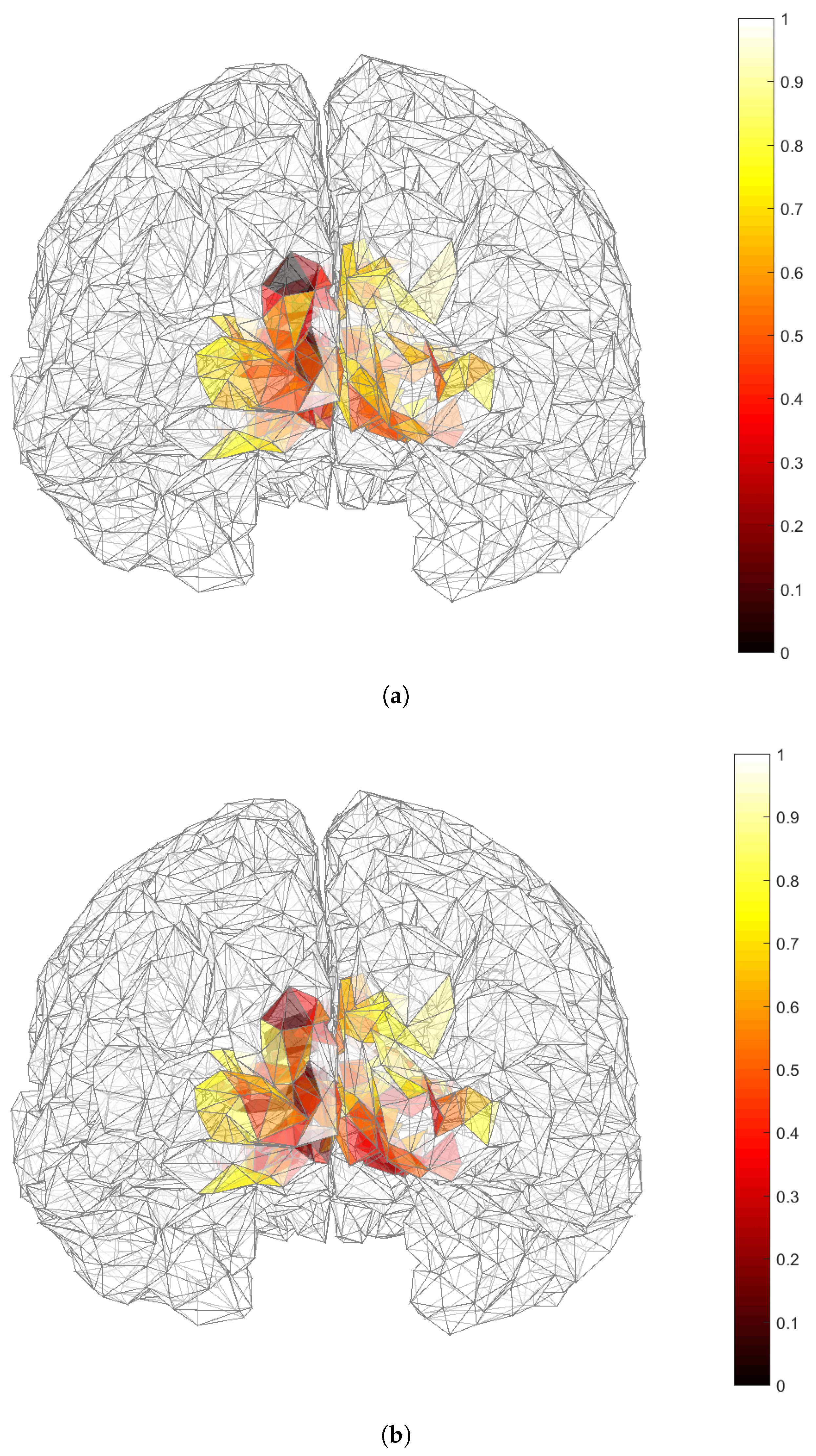
3.2. Applicability of and in Dipole Source Localization Using Real EEG Data
4. Discussion
5. Conclusions
Author Contributions
Funding
Institutional Review Board Statement
Informed Consent Statement
Data Availability Statement
Conflicts of Interest
References
- Asadzadeh, S.; Rezaii, T.Y.; Beheshti, S.; Delpak, A.; Meshgini, S. A systematic review of EEG source localization techniques and their applications on diagnosis of brain abnormalities. J. Neurosci. Methods 2020, 339, 108740. [Google Scholar] [CrossRef] [PubMed]
- Frost, O.T. An algorithm for linearly constrained adaptive array processing. Proc. IEEE 1972, 60, 926–935. [Google Scholar] [CrossRef]
- Van Veen, B.D.; van Drongelen, W.; Yuchtman, M.; Suzuki, A. Localization of Brain Electrical Activity via Linearly Constrained Minimum Variance Spatial Filtering. IEEE Trans. Biomed. Eng. 1997, 44, 867–880. [Google Scholar] [CrossRef]
- Sekihara, K.; Nagarajan, S.S. Adaptive Spatial Filters for Electromagnetic Brain Imaging; Springer Science & Business Media: Berlin, Germany, 2008. [Google Scholar]
- Belardinelli, P.; Ortiz, E.; Barnes, G.; Noppeney, U.; Preissl, H. Source reconstruction accuracy of MEG and EEG Bayesian inversion approaches. PLoS ONE 2012, 7, e51985. [Google Scholar] [CrossRef]
- Piotrowski, T.; Zaragoza-Martinez, C.C.; Gutiérrez, D.; Yamada, I. MV-PURE estimator of dipole source signals in EEG. In Proceedings of the 2013 IEEE International Conference on Acoustics, Speech and Signal Processing, Vancouver, BC, Canada, 26–31 May 2013; IEEE: New York, NY, USA, 2013. [Google Scholar]
- Gutiérrez, D.; Nehorai, A.; Dogandzic, A. Performance analysis of reduced-rank beamformers for estimating dipole source signals using EEG/MEG. IEEE Trans. Biomed. Eng. 2006, 53, 840–844. [Google Scholar] [CrossRef]
- Piotrowski, T.; Nikadon, J.; Moiseev, A. Localization of brain activity from EEG/MEG using MV-PURE framework. Biomed. Signal Process. Control 2021, 64, 102243. [Google Scholar] [CrossRef]
- Halder, T.; Talwar, S.; Jaiswal, A.K.; Banerjee, A. Quantitative evaluation in estimating sources underlying brain oscillations using current source density methods and beamformer approaches. Eneuro 2019, 6, 4. [Google Scholar] [CrossRef]
- Gaxiola-Tirado, J.A.; Salazar-Varas, R.; Gutiérrez, D. Using the partial directed coherence to assess functional connectivity in electroencephalography data for brain–computer interfaces. IEEE Trans. Cogn. Dev. Syst. 2017, 10, 776–783. [Google Scholar] [CrossRef]
- Piotrowski, T.; Nikadon, J.; Gutiérrez, D. MV-PURE spatial filters with application to EEG/MEG source reconstruction. IEEE Trans. Signal Process. 2018, 67, 553–567. [Google Scholar] [CrossRef]
- Chipman, J.S. Linear restrictions, rank reduction, and biased estimation in linear regression. Linear Algebra Its Appl. 1999, 289, 55–74. [Google Scholar] [CrossRef]
- Zaragoza-Martínez, C.C.; Gutiérrez, D. Electro/magnetoencephalography beamforming with spatial restrictions based on sparsity. Biomed. Signal Process. Control 2013, 8, 615–623. [Google Scholar] [CrossRef]
- Van Veen, B.D.; Buckley, K.M. Beamforming: A versatile approach to spatial filtering. IEEE ASSP Mag. 1988, 5, 4–24. [Google Scholar] [CrossRef] [PubMed]
- Jiménez-Cruz, E.; Gutiérrez, D. Reduced-rank beamforming for brain source localization in presence of high background activity. In Proceedings of the 2019 53rd Asilomar Conference on Signals, Systems, and Computers, Pacific Grove, CA, USA, 3–6 November 2019; IEEE: New York, NY, USA, 2019; pp. 2166–2170. [Google Scholar]
- Dogandzic, A. Minimum variance beamforming in low-rank interference. In Proceedings of the Thirty-Sixth Asilomar Conference on Signals, Systems and Computers, Pacific Grove, CA, USA, 3–6 November 2002; Volume 2, pp. 1293–1297. [Google Scholar]
- Herbordt, W.; Kellermann, W. Analysis of blocking matrices for generalized sidelobe cancellers for non-stationary broadband signals. In Proceedings of the 2002 IEEE International Conference on Acoustics, Speech, and Signal Processing, Orlando, FL, USA, 13–17 May 2002; IEEE: New York, NY, USA, 2002; Volume 4, p. IV–4187. [Google Scholar]
- Tivadar, R.I.; Murray, M.M. A primer on electroencephalography and event-related potentials for organizational neuroscience. Organ. Res. Methods 2019, 22, 69–94. [Google Scholar] [CrossRef]
- Muravchik, C.H.; Nehorai, A. EEG/MEC error bounds for a static dipole source with a realistic head model. IEEE Trans. Signal Process. 2001, 49, 470–484. [Google Scholar] [CrossRef]
- Van Trees, H.L. Optimum Array Processing. Detection, Estimation, and Modulation Theory; Wiley-Interscience: Hoboken, NJ, USA, 2002. [Google Scholar]
- Moiseev, A.; Gaspar, J.M.; Schneider, J.A.; Herdman, A.T. Application of multi-source minimum variance beamformers for reconstruction of correlated neural activity. NeuroImage 2011, 58, 481–496. [Google Scholar] [CrossRef] [PubMed]
- Gutiérrez, D.; Nehorai, A.; Dogandzic, A. MEG source estimation in the presence of low-rank interference using cross-spectral metrics. In Proceedings of the 26th Annual International Conference of the IEEE Engineering in Medicine and Biology Society, San Francisco, CA, USA, 1–5 September 2004; IEEE: New York, NY, USA, 2004; Volume 3, pp. 990–993. [Google Scholar]
- Goldstein, S.; Reed, I. Subspace selection for partially adaptive sensor array processing. IEEE Trans. Aerosp. Electron. Syst. 1997, 33, 539–544. [Google Scholar] [CrossRef]
- Bronez, T. Sector interpolation of non-uniform arrays for efficient high resolution bearing estimation. In Proceedings of the International Conference on Acoustics, Speech, and Signal Processing, New York, NY, USA, 11–14 April 1988; pp. 2885–2886. [Google Scholar]
- de Munck, J.C.; Vijn, P.C.; da Silva, F.L. A random dipole model for spontaneous brain activity. IEEE Trans. Biomed. Eng. 1992, 39, 791–804. [Google Scholar] [CrossRef]
- Dogandzic, A.; Nehorai, A. Estimating evoked dipole responses in unknown spatially correlated noise with EEG/MEG arrays. IEEE Trans. Signal Process. 2000, 48, 13–25. [Google Scholar] [CrossRef]
- Georgiadis, K.; Liaros, G.; Oikonomou, V.P.; Chatzilari, E.; Adam, K.; Nikolopoulos, S.; Kompatsiaris, I. Multimedia Authoring and Management EEG SSVEP Dataset I. 2016. Available online: https://figshare.com/articles/dataset/MAMEM_EEG_SSVEP_Dataset_I_256_channels_11_subjects_5_frequencies_/2068677 (accessed on 2 February 2023).
- Oikonomou, V.P.; Liaros, G.; Georgiadis, K.; Chatzilari, E.; Adam, K.; Nikolopoulos, S.; Kompatsiaris, I. Comparative evaluation of state-of-the-art algorithms for SSVEP-based BCIs. arXiv 2016, arXiv:1602.00904. [Google Scholar]
- Diwakar, M.; Huang, M.X.; Srinivasan, R.; Harrington, D.L.; Robb, A.; Angeles, A.; Muzzatti, L.; Pakdaman, R.; Song, T.; Theilmann, R.J.; et al. Dualcore beamformer for obtaining highly correlated neuronal networks in MEG. NeuroImage 2011, 54, 253–263. [Google Scholar] [CrossRef]
- Di Russo, F.; Pitzalis, S.; Aprile, T.; Spitoni, G.; Patria, F.; Stella, A.; Spinelli, D.; Hillyard, S.A. Spatiotemporal analysis of the cortical sources of the steady-state visual evoked potential. Hum. Brain Mapp. 2007, 28, 323–334. [Google Scholar] [CrossRef] [PubMed]
- Wu, Z. Physical connections between different SSVEP neural networks. Sci. Rep. 2016, 6, 22801. [Google Scholar] [CrossRef] [PubMed]
- Allison, B.Z.; Wolpaw, E.W.; Wolpaw, J.R. Brain–computer interface systems: Progress and prospects. Expert Rev. Med Devices 2007, 4, 463–474. [Google Scholar] [CrossRef] [PubMed]


| Variable/Notation | Description |
|---|---|
| lth dipole source | |
| L | number of dipoles |
| Q | matrix containing all dipole sources |
| time-varying magnitudes of lth dipole’s Cartesian components | |
| N | total number of time samples |
| vector representing a position (Cartesian coordinates) | |
| volume of the brain | |
| lth dipole’s position | |
| matrix containing all L dipole’s positions (parameter of interest) | |
| time-varying EEG measurement at the mth sensor | |
| M | total number of sensors |
| matrix with all EEG measurements at the kth experiment (trial) | |
| K | total number of independent trials |
| lth lead field matrix associated to the lth dipole’s position | |
| matrix comprising the L lead field matrices as a function of | |
| measurement noise realization in the mth sensor at time t | |
| variance of measurement noise | |
| matrix with all measurement noise at the kth trial | |
| indicates a consistent estimate of Z | |
| W | spatial filter (beamformer) |
| I | identity matrix |
| matrix full of zeros | |
| indicates an approximation of Q | |
| approximated dipoles at the kth trial | |
| lead field matrix as a function of | |
| beamformer as a function of | |
| linearly constrained minimum variance (LCMV) beamformer | |
| R | data covariance matrix |
| P | noise covariance matrix |
| LCMV-based neural activity index (NAI) as a function of | |
| multi-source activity index (MAI) as a function of | |
| reciprocal of the noise power as a function of | |
| reciprocal of the sources’ power as a function of | |
| generalized sidelobe canceler (GSC) | |
| quiescent component of the GSC | |
| noise-plus-interference components of the GSC | |
| blocking matrix | |
| projection matrix of A | |
| undesired measurement components | |
| autocorrelation matrix of the undesired signals | |
| Wiener filter that minimizes the mean-squares of | |
| matrix containing all undesired signals | |
| first proposed reduced-rank (RR) NAI a function of | |
| RR approximation of | |
| eigenvalues of | |
| orthonormal eigenvectors of | |
| second proposed RR-NAI as a function of | |
| cross-correlation of and | |
| matrix with all positions of interference sources | |
| lead field matrix as a function of | |
| matrix containing all interference dipole sources | |
| variance of biological noise | |
| signal-to-measurement-noise ratio | |
| signal-to-biological-noise ratio | |
| matrix containing candidate dipole’s positions | |
| bias of the estimate of at the kth trial | |
| sum-of-squares of at the kth trial | |
| maximum bias at the kth trial | |
| average sum-of-squares | |
| standard deviation of the maximum bias | |
| minimum power of |
Disclaimer/Publisher’s Note: The statements, opinions and data contained in all publications are solely those of the individual author(s) and contributor(s) and not of MDPI and/or the editor(s). MDPI and/or the editor(s) disclaim responsibility for any injury to people or property resulting from any ideas, methods, instructions or products referred to in the content. |
© 2023 by the authors. Licensee MDPI, Basel, Switzerland. This article is an open access article distributed under the terms and conditions of the Creative Commons Attribution (CC BY) license (https://creativecommons.org/licenses/by/4.0/).
Share and Cite
Jiménez-Cruz, E.; Gutiérrez, D. Interference Suppression in EEG Dipole Source Localization through Reduced-Rank Beamforming. Appl. Sci. 2023, 13, 3241. https://doi.org/10.3390/app13053241
Jiménez-Cruz E, Gutiérrez D. Interference Suppression in EEG Dipole Source Localization through Reduced-Rank Beamforming. Applied Sciences. 2023; 13(5):3241. https://doi.org/10.3390/app13053241
Chicago/Turabian StyleJiménez-Cruz, Eduardo, and David Gutiérrez. 2023. "Interference Suppression in EEG Dipole Source Localization through Reduced-Rank Beamforming" Applied Sciences 13, no. 5: 3241. https://doi.org/10.3390/app13053241
APA StyleJiménez-Cruz, E., & Gutiérrez, D. (2023). Interference Suppression in EEG Dipole Source Localization through Reduced-Rank Beamforming. Applied Sciences, 13(5), 3241. https://doi.org/10.3390/app13053241