Abstract
Excitation identification for nonlinear structures is still a challenging problem due to the convergence and accuracy in this process. In this study, a load estimation method is proposed with orthogonal decomposition, the order for which can be fairly accurately determined by a regression. In this process, the force time history is represented by the orthogonal basis and the coefficients of the orthogonal decomposition are taken as unknowns and augmented to the state variable, which can be identified recursively in state space. A general energy-conserving method is selected to a step-by-step integration to guarantee the convergence of this integration. The proposed method is first validated by numerical simulation studies of a truss structure considering its geometric property. The identification results of the numerical studies demonstrate that the proposed excitation identification method and the orthogonal decomposition order determination method work well for nonlinear structures. The laboratory work of a 7-story frame is investigated to consider the geometric nonlinearity in impact force identification. The results of experimental studies show that uncertainties such as measurement noise and model error are included in the investigation of the accuracy and robustness of the proposed force identification method, while the time history of external forces could be identified with promising results.
1. Introduction
Load estimation of severe environmental excitation, such as an earthquake or strong wind, is of great significance in structural design, health monitoring, and condition assessment. Under the practical condition, the external forces of structures cannot be directly measured with force transducers due to the limited number of sensors or an inaccessible force position [1]. Therefore, inverse dynamic analysis is an alternative tool to estimate an external force or excitation with structural response observation, which may be ill-conditioned [2,3]. Currently, investigations on the dynamic load estimation are being conducted more frequently, but it is still a difficult task for nonlinear structures due to nonlinearity, performance of time-step integration method, and the measurement noise.
Numerous indirect force re-construction or force identification methods have been developed for linear structures [4,5,6,7,8,9]. Force identification methods in time domain are actively studied in state space with the time history of structural response as the measured information which can be solved with iterative regularization methods, recursive estimation or some other optimization methods [10,11,12,13,14]. Force identification can also be viewed as an optimization problem the objective of which is to minimize the error between the measured and the estimated structural responses.
Compared to the force identification method arranged in one unknown vector solved with regularization method in state space [15], it has been argued that state variables estimated in state space recursively can identify the external force with far fewer unknowns in each time step as introduced in references [16,17,18,19]. The extended Kalman filter (EKF) has been developed as an effective estimation tool to identify the state variable, including the structural response, parameters, and external excitation [17,18]. This filter can also be applied and combined with least-square estimation to identify the structural parameter and external load recursively with an adaptive factor [20,21]. To improve accuracy of the nonlinear structural estimation, the unscented Kalman filter (UKF) was proposed with fewer deterministic samplings than the particle filters or other ensemble Kalman filters [19,22,23,24], which will improve computational efficiency. Compared to EKF, it is unnecessary to calculate the Jacobian matrix in the identification process with UKF. Therefore, UKF is a suitable tool to conduct a time-invariant constitutive parameter or nonlinear structural parameter identification for nonlinear civil buildings.
In the studies of force identification, the unknown time history of external force or ground motion can be augmented to a state variable [16,17,18,19]. UKF methods have been used for the augmented state variable estimation combined with response or structural parameters. It should be noted that UKF is not suitable for the identification of a time-variant parameter when the dynamic external force or ground motion is a time-variant series. The force identification with a directly augmented state variable may not be as accurate as the time-invariant structural parameter identification. The factor mentioned above could cause large errors in the identification result, especially considering the time-variant statistical characteristics of the external excitation. Chebyshev polynomial decomposition of the time history was proposed [25]. The force time history is assumed to be represented by the Chebyshev polynomials whose coefficients are arranged as a very large vector and identified in state space with regularization methods, as reported in reference [25]. However, it is difficult to determine the order of the polynomial when there is little information about an external excitation. Compared with the generally used Fourier decomposition, the Chebyshev basis would cover a wide range in frequency for each single basis, which could reduce the number of bases and the corresponding coefficients. Until now, only a fraction of force identification methods for nonlinear structures have been concerned with estimating the force identification or simultaneous identification problems for nonlinear structures based on nonlinear recursive estimation tools.
In the force identification process, a dynamic analysis with a finite element model of the structure is usually required to obtain numerical structural responses. The time integration method is an efficient numerical tool for the response simulation of a large-scale structural system and structural dyanmic testing [26,27,28,29,30,31]. The step-by-step integration method can also be divided into two classes: explicit and implicit methods. For instance, central differentiation method is a commonly used explicit integration method while it is conditionally stable. Implicit step-by-step integration method is an alternative tool to solve the equation of motion, which is unconditionally stable. It should be noted that the stability performance mentioned above is related to linear, but not nonlinear structures. The convergence performance of the implicit nonlinear dynamic analysis is totally different and it is difficult to guarantee convergence for the nonlinear dynamic analysis. Therefore, a forward and inverse dynamic analysis may be inaccurate or even unstable due to the nonlinearities, including hysteresis and geometric nonlinearity which exist in structures. Selecting a time integration method for the inverse dynamic analysis of a nonlinear structural system will also influence the accuracy and stability of the analysis. The energy-conserving integration method (ECIM), has been proposed [26,27,28,29], especially for geometric nonlinearity, but, until now, it has never been concerned about the inverse dynamic problem which renders the inverse analysis inaccurate.
In this paper, a force identification method is proposed for nonlinear structures. A general version of ECIM was developed and applied to the inverse dynamic analysis when considering structural nonlinearity. In the dynamic analysis of structures with geometric nonlinearity, the physical matrices of the structures are time variant, because the small deformation hypothesis cannot work in this condition. Without the optimization methods in this study, the convergence of the dynamic analysis would influence the inverse analysis adversely. ECIM was selected to solve the problem in this study to ensure convergence of the dynamic analysis. In the process of dynamic load identification, it is recognized that there are a large number of unknowns in force time history which could have an adverse effect on identification results. A Chebyshev polynomial decomposition method was utilized for the external force identification of nonlinear structures. The order of Chebyshev polynomials was determined using a practical method based on frequency analysis of the structural response, from which a formulation was obtained with regression to determine the decomposition order. Numerical simulation was conducted with a two-dimension truss structure and a base isolated building. The load identification method has also been validated by experimental studies of a seven-story plane frame, a series of quasi-static tests of full-scale rubber isolation and hybrid simulation of a nonlinear isolated structure. Structural uncertainties in materials, unexpected ground motion, and measurement noise are considered to validate the robustness of the proposed method.
2. Equation of Motion and Its Solution Considering Structural Nonlinearity
The equation of motion of an N degree-of-freedom damped linear structural system subjected to external excitation can be represented as
where M, C, and K are the mass, damping, and stiffness matrices of the structural system, respectively. F is the vector of external excitation forces on the structure and L is the mapping matrix for the input forces. , , and are vectors of acceleration, velocity, and displacement of the structural system, respectively. The Rayleigh damping model was used in this study and assumed with Equation (2)
where a1 and a2 are the Rayleigh damping coefficients.
When the structural system is nonlinear, the discrete equation of motion can be represented with
where Rk(x) is the restoring force of the structure which is a nonlinear function of the displacement and k represents the integration time step. When the structure is subjected to seismic excitation, the equation of motion for nonlinear structure becomes
where is the acceleration at ground level. The Newmark-β method can be used to solve the response of linear system shown in Equation (1) with the following assumption:
where represents the time interval in the integration.
The Newmark-β method for a linear structural system can be extended to solve Equations (3) and (4) representing a nonlinear system. The time-step solution with the Newmark-β method was commonly used, however, it was found that the Newmark-β method cannot guarantee stability in the case of geometric nonlinearity [26,27]. To improve the accuracy and stability of the dynamic analysis, a new equation of motion in discrete form is provided in the middle of each time step instead of Equation (3) or Equation (4) with the following assumption:
where Fm, vm, and Rm are the average external force, velocity, and resisting force between the k and k + 1 time step with the definition as follows
The new equation of motion in the mid-point between the time step of k and k + 1 for the structure subjected to the external force becomes
Based on the assumption in Equation (5), the following equation can be obtained:
Substitute Equation (11) into both sides of Equation (10) multiplied by the increment of the displacement , and a new equation will be obtained as follows.
Equation (12) makes the dynamic analysis relate to the energy of the structural system. Equation (12) illustrates the energy transfer and dissipation in the system. Based on Equation (12) it can be proved that with the assumptions shown in Equations (6) and (7), both the equation of motion and the energy conserving of the system considering the work of the input force or excitation will be satisfied. The ECIM was first proposed by Simo and Tarnow [26] to improve the implicit mid-point integration method for nonlinear structures with the characteristic that the term of Rn,m was calculated with a new version considering the concept of energy conserving for the structural system. Beam and truss structures were used as an example of ECIM for the dynamic analysis, [25,28] which is also applied in this paper when geometric nonlinearity is considered. The general version of the method is developed as Equation (12) which is applied to solve the equation of motion both for the forward and inverse dynamic problem.
3. Force Identification in State Space
3.1. Joint Estimation in State Space
In the forward dynamic analysis, the state space equation of the nonlinear structural system shown in Equation (3) can be expressed generally as Equation (13).
where X denotes the state vector including , u is the input of the system, wk−1 is the system process noise vector, and F is a nonlinear function of state vector X. It is noted that Equation (1) can also be expressed in state space as Equation (3). The discrete observed function can be written as
where v represents the observation noise assumed to follow a Gaussian white noise with zero mean and a covariance matrix R. The identification process can be initialized with the guess of X0 = E[X] and based on unscented Kalman filter or other nonlinear estimators [22,23,24].
External excitations are always unknown for practical inverse problems. When the external load is unknown, the state equation of nonlinear hysteresis structural system cannot be solved with Equation (13). It is always difficult to directly identify the external force of nonlinear structure with UKF since it may be nonstationary and time variant. It is also impossible to build a relationship between ‘fk’ and ‘fk−1′ of external excitation but the excitation F can be decomposed on a determined standard orthogonal basis. Since the orthogonal basis is known, the history of excitation will be re-constructed as if the coefficients of orthogonal basis can be identified. In this way, the external excitation identification is transformed to the identification of the coefficients of orthogonal decomposition. The excitation in Equation (1) can be decomposed as follows
in which is the weighing coefficient of polynomial . High order components in polynomials are ignored for the purpose of computational efficiency. Low frequency components in excitation would be a major contribution to the structural response for civil engineering structures. is the mth term orthogonal polynomial. Nm is the number of the term of input decomposition which is also derived from the order of the decomposition. The orthogonal polynomial and order of the decomposition Nm can affect the accuracy of input approximation. The order of input decomposition Nm is closely related to the input history length and concerned bandwidth of the external excitation in the frequency domain. The orthogonal polynomial can be determined with different kinds of decomposition methods. In this paper the Chebyshev orthogonal polynomial is utilized for the decomposition and can be written as follows.
where Nm is the order of decomposition. Based on the Chebyshev polynomial standard orthogonal polynomial decomposition, Equation (1) can be rewritten as follows:
where Nf is the number of the external excitation. The external excitation is approximated by the Chebyshev polynomial. To re-construct the external force accurately, the order of the Chebyshev polynomial should be determined and the polynomial parameter is required to be identified accurately. In the force identification problem, the state space equation of the nonlinear structural system with unknown input can then be rewritten as
where is a part of process noise. The coefficients of Chebyshev basis augmented in the state variable can be identified by the UKF introduced in references [17,19,22,23,24]. When the parameters of a nonlinear structural system must be identified, the unknown parameters can be augmented to the state variable of the state space as shown in Equation (18). In this paper, the accurate identification of the external force is the focus and the observability for the force identification can relate to reference [17].
3.2. Determination of the Order for the Orthogonal Decomposition
Before the identification of the coefficients of the Chebyshev basis, the determination of the Chebyshev polynomial order is of great importance. To discuss the order of the Chebyshev polynomial, the first two, six, ten, fifteen and twenty terms of Chebyshev polynomial for 3 s are first selected and shown in Figure 1. Here, it can be seen that the characteristics of the Chebyshev polynomials, including peaks and valleys, are a little similar to Fourier series, so this can be used to represent the periodic signal or the signal consisting of periodic components. It is also helpful to conduct a frequency analysis of the measured structural response which depends on the property of the external load.

Figure 1.
Re-construction of single frequency signals with Chebyshev polynomial.
An example is first provided to demonstrate that the periodic signal can be represented by the Chebyshev polynomials as follows. A one second sine wave with the frequency at 1 Hz is shown in Figure 2. To solve the coefficients for the re-construction of the signal, Equation (15) can be rewritten as follows:
where T represents the determined Chebyshev polynomial basis and W denotes the unknown vector of the Chebyshev polynomials. The coefficients vector can be solved with the following bounds to this re-construction problem as
where λ is the non-negative damping coefficient governing the participation of the least-squares error in the solution. Solving Equation (20) is equivalent to minimizing the following function
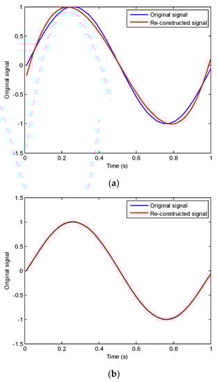

Figure 2.
Re-construction of single frequency signals with Chebyshev polynomial. (a) Re-construction with first five terms of Chebyshev polynomial. (b) Re-construction with first six terms of Chebyshev polynomial. (c) Re-construction with first nine terms of Chebyshev polynomial. (d) Re-construction with first ten terms of Chebyshev polynomial. (e) Re-construction with first forty terms of Chebyshev polynomial.
With the solution to Equation (21), the re-constructed signals are compared with the original signals as shown in Figure 2. First, the single period sine wave is constructed with the first five terms and six terms of Chebyshev polynomials. The re-construction results are shown in Figure 2a,b, where a one-period sine wave can be represented by the first sixth-term of Chebyshev polynomials accurately while the error is a little larger based on the five-term re-construction. Then, the re-construction of another sine wave is conducted the results of which are shown in Figure 2c,d. Here, we can see in the figure that ten terms of polynomials perform better than the nine-term Chebyshev polynomial re-construction. The conclusion is similar in that the bandwidth of the summation of the polynomials should cover the bandwidth of the original signal. Lastly, the investigation of a sine wave signal with 10 periods is conducted and decomposed by Chebyshev polynomials. The re-construction results are shown in Figure 2e, which clearly shows that the signal can be decomposed with 42-term Chebyshev polynomials accurately. The re-construction errors of the sine waves for the results in Figure 2 are listed in Table 1. From the results shown in Figure 2 and Table 1, it can be concluded that the order of Chebyshev polynomials is only related to the number of the period for the single frequency signal and the required number of order is nearly four times of the number of the period. It can also be deduced that there is a relation between the number of periods in signal and the number of terms in the Chebyshev polynomial decomposition. A brief conclusion can also be drawn that the combined bandwidth of the polynomials should cover the bandwidth of the original signal. In other words, the frequency of the higher order of Chebyshev polynomial decomposition should at least exceed the concerned upper limit of the bandwidth of the signal. In this way, the Fourier basis used for the decomposition compared to the polynomials will result in a large number of unknowns to cover the bandwidth of the excitation signal. This is also the reason the Chebyshev polynomial was selected to conduct the decomposition in this study.

Table 1.
Error of the Re-construction with different order Chebyshev polynomial.
Multi-frequency signal can also be decomposed with Chebyshev polynomials. The highest order of the polynomial used in the decomposition can be approximately determined by the highest frequency of the signal, which is similar to decomposition of the single frequency signal. The Chebyshev decomposition can be expanded to the random signals. Generally, a random signal can be taken as the summation of the periodic signals which can also be decomposed with Chebyshev polynomials. The order of the Chebyshev polynomial will depend on the highest frequency concerned and the length of the signal. Another example is provided to demonstrate the decomposition of multi-frequency signals. A four-second signal defined as a summation of sine waves F = 0.2 × sin(2πt) + 0.05 × sin(6πt) + 0.03 × sin(9πt) + 4. The frequency analysis based on fast Fourier transform is shown in Figure 3. The frequency analysis result is shown in Figure 3a. The highest frequency is 4.5 Hz and other two frequencies are approximately 2.93 Hz and 0.98 Hz. Therefore, the order of the highest Chebyshev polynomial can be determined as α × 4.5 × 4. The value of α can be determined through the inverse study as shown in Equation (22) and varies with the number of the periods ‘np’ in the signal. The formulation for α is shown as follows.
where α is obtained with the general curve fitting method based on the first order approximation. With the determined highest order of Chebyshev polynomial, the signal is re-constructed as shown in Figure 3b. The Chebyshev polynomial can accurately re-reconstruct the original signal. The weighing coefficients of the Chebyshev decomposition exist as long as the highest order of the polynomial can be stably determined. It is also expected that the coefficients of the Chebyshev polynomial can be identified with a suitable identification tool in the force identification problem. The random excitation is a special kind of multi-frequency load which may be applied on structures. Although it is difficult for the random signal to be represented by Chebyshev polynomials with only very few terms, this paper will provide an approximation method to evaluate the crucial component in the random excitation for the structure as introduced in the numerical study.
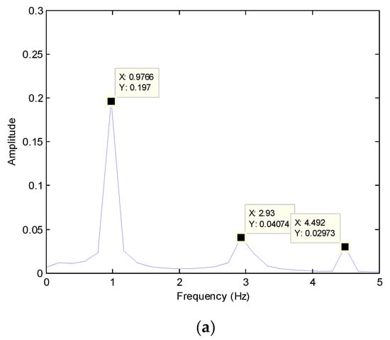

Figure 3.
Re-construction of multi-frequency signals with Chebyshev polynomial. (a) Frequency analysis of the signal. (b) Re-construction based on the frequency analysis.
4. Numerical Studies
In the numerical studies, structures with two typical nonlinearity will be investigated, namely, a truss structure considering the geometric nonlinear properties and a base isolated frame considering the nonlinear hysteretic property of the base isolation layer. The load identification error is defined in this paper as
where the subscript true represents the true load or ground motion, ‘id’ means the identification time history. The identification can be performed iteratively for better accuracy and the convergence criteria Tol in the iteration procedure is set as
where i denotes the number of the iteration and Tol is taken as 10−3.
A two-dimensional 40 m long truss structure is shown in Figure 4. The structural deformation is large, so the influence of a large deformation on internal force cannot be ignored. This truss structure consists of 161 truss elements and 82 nodes, each of which has two degrees of freedom. It is assumed that the two ends of each truss element are hinged and the boundary condition of this long span truss structure also supported at two end nodes with hinges. The length of chord members and the vertical web members is 1 m, while the length of other web members is m. Young’s modulus and the area of the truss element are E = 2 × 10⁵ Mpa and 100 mm2, respectively.

Figure 4.
Truss structure.
In the forward dynamic analysis of the truss structure, the initial vertical velocity of Nodes 39, 41, and 43 was set as 50 m/s and other initial responses of the structure as zero. The damping ratio of each mode was set as zero to validate the stability of the time integration method. The dynamic response analysis for the free vibration of the truss structure was studied. In the dynamic analysis process, the physical matrices, including mass matrix and stiffness matrix are time-variant matrices obtained based on finite element technology considering the large deformation caused by the large initial velocity. The structural response on Node 41 calculated with Newmark-β method is compared with the result from the ECIM as shown in Figure 5. Here, Figure 5 illustrates that the response solved by Newmark-β method diverges around 4.29 s while the response solved by ECIM converges, although in the result before 4 s the two responses nearly overlap. The energy of the system evaluated based on Equation (11) with different calculated structural responses is compared in Figure 6. Here, it is revealed that the energy of the system solved by ECIM is nearly a constant. The increasing energy is the reason for the divergence of the response solved by Newmark-β. Therefore, it is possible to use ECIM as an alternative method for the dynamic analysis of the forward and inverse problems.

Figure 5.
Displacement time history of the free vibration with different integration methods.

Figure 6.
Energy of the system with different time integration methods.
In the numerical study of the force identification for this nonlinear truss structure, a multi-frequency force was applied on the Node 39 which will be identified by the proposed identification method with orthogonal decomposition. The applied force is expressed as F = sin(6πt) + sin(11πt) and the lasting time for the external force is taken as 3 s. To simulate the effect of measurement uncertainty, Gaussian white noise was added to the uncorrupted acceleration time history computed from the finite element model.
Based on the frequency analysis of the structural response, the frequency of the highest most concerned frequency with peak picking method is 5.35 Hz with the fast Fourier transform. Under this condition the order of the Chebyshev polynomial is then 55, which is obtained with the approximation formulation of 3.37 × 5.35 × 3 ≈ 55. The vertical acceleration of Nodes 20 to 30 was used as measured data. The external force identification results are shown in Figure 7. It is demonstrated that the external load can be accurately identified when using the proposed methods, even considering the geometric nonlinearity. When 5% noise is factored into the measurement, the identification result is also fairly accurate even though more fluctuations exist in the peak. Due to its special requirements the error can also be mitigated by the higher order as is shown by the analysis results in Table 1. The proposed practical order selection method can work well based on the validation of this case.

Figure 7.
Identification of multi-frequency external force considering geometric nonlinearity. (a) Force identification result without measurement noise. (b) Force identification result with 5% measurement noise.
5. Laboratory Validation
Nonlinearity is considered in the experimental studies and validation. A 7-story plan frame considering geometric nonlinearity was studied with rigid boundary condition and the impact force on the top story identified. The vibration of a planar flexible seven-story steel frame was investigated considering the geometric nonlinearity. This frame was fabricated in the laboratory of the Hong Kong Polytechnic University [11] and the impact force identified based on the method proposed in Section 3. The height of each story is 300 mm and the length of the beam on each story is 500 mm. In this study, the displacement-based fiber element was used to model the beam and column components while geometric nonlinearity was factored in due to flexibility of the structure. During the test, the frame retained elastic performance because the impact force was not that large. Two lumped masses were placed on each story of the frame on the 1/4 length and 3/4 length of the beam to simulate the mass effect of the floor slab, and the weight of each lumped mass was around 3.95 kg. The ends of the columns in the first story were welded to a thick steel base plate which was connected rigidly to the ground. The planar frame was made of Q235 steel. The areas of the beam and column section are 49.98 mm × 8.92 mm and 49.89 mm × 4.85 mm, respectively. The primary parameters of the model consist of modulus of elasticity (E = 206 GPa), Poisson ratio (υ = 0.31), initial yield strength (fy = 235 MPa), post yield stiffness ratio (b = 0.02), and density (ρ = 7.85 g/cm3). All the parameters above are taken as known parameters in the force identification process and were obtained with material test data.
In the experimental study, the external force of this structure was a horizontal impact force on the plan of structure on the top floor with a force hammer. Acceleration responses of the frame were recorded by DEWESoft software and NI data acquisition with a sampling rate of 1000 Hz. The tested Young’ modulus of beam and column are 2.2 × 10¹¹ N/m2 and 1.9 × 10¹¹ N/m2, respectively. The horizontal acceleration responses recorded on the 1st, 3rd, 5th, 6th, and 7th stories were used to estimate the impact force based on ECIM. The first 300 sampling data performs as a window for the impact force estimation. Due to the large deformation caused by the impact force, the geometric property of the frame behavior is considered by the time-variant physical matrices of the frame.
The comparison of the measured impact force by force transducer and the identified force is shown in Figure 8 and Figure 9 with/without a time window to modify the identification results. When the time window is used, the time window is set as 0.1 s considering the very short interaction time. It is noted that the impact force can be represented by triangle signal or sine wave in previous studies which can determine the order of the decomposition directly in this special case. The 7th order of Chebyshev polynomial was used in the former case with a time window and 14th order used in latter identification case without a time window. These two figures show that the peaks of the identified impact force time are very close to the peak of the measured force, but the identification without a time window contains some fluctuations. The identification error in the comparison may also result from the direction of the impact force on the top story. The comparison of these two results indicates that a time window can improve the identification accuracy and reduce the number of unknowns in a state variable. The result also indicates that the identification result is more accurate when considering the geometric nonlinearity of these kinds of flexible frame, than the identification result that ignores the geometric nonlinearity in reference [11].

Figure 8.
Impact force identification with time window.

Figure 9.
Impact force identification without time window.
6. Conclusions
In this study a new force estimation method is proposed with orthogonal decomposition based on a UKF algorithm for geometric nonlinear structures. The practical method ECIM was selected and used to determine the decomposition order, and was also proposed to account for the regression error. The proposed method was verified with simulation and experimental studies. The results show that, compared to the traditional step-by-step integration method, the ECIM can guarantee the convergence of the dynamic inverse analysis process. With the frequency analysis of the measurement and the proposed load estimation method, the decomposition order for external force is reasonable as the external force can be identified accurately, even with the measurement noise. When geometric nonlinearity is considered in flexible structures, the load estimation result is more accurate. The initial value of orthogonal decomposition could also influence the identification result and this problem will be solved in future work.
Author Contributions
Conceptualization, L.G. and Y.D.; methodology, Y.D.; software, Y.D.; validation, L.G.; formal analysis, L.G.; investigation, L.G.; resources, Y.D.; data curation, L.G.; writing—original draft, L.G. and Y.D.; writing—review and editing, L.G.; supervision, L.G.; project administration, Y.D.; funding acquisition, Y.D. All authors have read and agreed to the published version of the manuscript.
Funding
The work in this paper was supported by the Scientific Research Fund of Institute of Engineering Mechanics, China Earthquake Administration (Grant No. 2019D24) and the 2018 Dongnong scholar program of Northeast Agricultural University: “Young Talents” (18QC31). The research is also supported by open subject of traffic Safety and Control lab in Hebei Province (No. JTKY2022002) and project (No. YC-201920) of the Transportation Department of Hebei Province.
Institutional Review Board Statement
Not applicable.
Informed Consent Statement
Not applicable.
Data Availability Statement
Not applicable.
Acknowledgments
Thanks to Y.Z. Zhang of Shijiazhuang Tiedao University, Z.G. Zhang, and J.J. Li of Yan Chong Highway Administration for their help, work, and contribution to this paper.
Conflicts of Interest
The authors declare no conflict of interest.
References
- Uhl, T. Identification of loads in mechanical structures-helicopter case study. Comput. Assist. Mech. Eng. Sci. 2002, 9, 151–160. [Google Scholar]
- Steltzner, A.D.; Kammer, D.C. Input force estimation using an inverse structural filter. In Proceedings of the 17th International Modal Analysis Conference, Kissimmee, FL, USA, 8–11 February 1999; pp. 954–960. [Google Scholar]
- Starkey, J.M.; Merrill, G.L. On the ill-conditioned nature of indirect force measurement techniques. Int. J. Anal. Exp. Modal Anal. 1989, 4, 103–105. [Google Scholar]
- Inoue, H. Review of inverse analysis for indirect measurement of impact force. Appl. Mech. Rev. 2001, 54, 503–524. [Google Scholar] [CrossRef]
- Uhl, T. The inverse identification problem and its technical application. Arch. Appl. Mech. 2007, 77, 325–337. [Google Scholar] [CrossRef]
- Green, M.F.; Cebon, D. Dynamic response of highway bridges to heavy vehicle loads: Theory and experimental validation. J. Sound Vib. 1994, 170, 51–78. [Google Scholar] [CrossRef]
- Chen, Z.; Chan, T. A truncated generalized singular value decomposition algorithm for moving force identification with ill-posed problems. J. Sound Vib. 2017, 401, 297–310. [Google Scholar] [CrossRef]
- Lai, T.; Yi, T.H.; Li, H.N. Parametric study on sequential deconvolution for force identification. J. Sound Vib. 2016, 377, 76–89. [Google Scholar] [CrossRef]
- Chan, T.; Yu, L.; Law, S.S. Comparative study on moving force identification: From bridge strains in laboratory. J. Sound Vib. 2002, 235, 87–104. [Google Scholar] [CrossRef]
- Liu, J.; Han, X.; Jiang, C.; Ning, H.; Bai, Y. Dynamic load identification for uncertain structures based on interval analysis and regularization method. Int. J. Comput. Methods 2011, 8, 667–683. [Google Scholar] [CrossRef]
- Ding, Y.; Law, S.S.; Wu, B.; Xu, G.X.; Lin, Q.; Jiang, H.B.; Miao, Q.S. Average acceleration discrete algorithm for force identification in state space. Eng. Struct. 2013, 56, 1880–1892. [Google Scholar] [CrossRef]
- Law, S.S.; Fang, Y.L. Moving force identification: Optimal state estimation approach. J. Sound Vib. 2001, 239, 233–254. [Google Scholar] [CrossRef]
- Busby, H.R.; Trujillo, D.M. Optimal regularization of an inverse dynamics problem. Comput. Struct. 1995, 63, 243–248. [Google Scholar] [CrossRef]
- Dobson, B.J.; Rider, E. A review of the indirect calculation of excitation forces from measured structural response data. Proc. Inst. Mech. Eng. Part C J. Mech. Eng. Sci. 1990, 204, 69–75. [Google Scholar] [CrossRef]
- Lourens, E.; Reynders, E.; DeRoeck, G.; Degrande, G.; Lombaert, G. An augmented Kalman filter for force identification in structural dynamics. Mech. Syst. Signal Process. 2012, 27, 446–460. [Google Scholar] [CrossRef]
- Ding, Y.; Zhao, B.Y.; Wu, B.; Xu, G.X.; Lin, Q.; Jiang, H.B.; Miao, Q.S. A Condition Assessment Method for Time-variant Structures with Incomplete Measurements. Mech. Syst. Signal Process. 2015, 58, 228–244. [Google Scholar] [CrossRef]
- Naets, F.; Cuadrado, J.; Desmet, W. Stable force identification in structural dynamics using Kalman filtering and dummy-measurements. Mech. Syst. Signal Process. 2015, 50–51, 235–248. [Google Scholar] [CrossRef]
- Radhikaa, B.; Manohar, C.S. Dynamic state estimation for identifying earthquake support motions in instrumented structures. Earthq. Struct. 2013, 5, 359–378. [Google Scholar] [CrossRef]
- Astroza, R.; Ebrahimian, H.; Li, Y.; Conte, J.P. Bayesian nonlinear structural FE model and seismic input identification for damage assessment of civil structures. Mech. Syst. Signal Process. 2017, 93, 661–687. [Google Scholar] [CrossRef]
- Li, Y.; Wu, Y.; Li, T. Identification of Nonlinear Structural Parameters Under Limited Input and Output Measurements. Int. J. Non-Linear Mech. 2012, 47, 1141–1146. [Google Scholar] [CrossRef]
- Yang, J.N.; Lin, S. On-line identification of non-linear hysteretic structures using an adaptive tracking technique. International. J. Non-Linear Mech. 2004, 39, 1481–1491. [Google Scholar] [CrossRef]
- Julier, S.J.; Uhlmann, J.K.; Durrant-Whyte, H.F. A new approach for filtering nonlinear systems. In Proceedings of the 1995 American Control Conference—ACC’95, Seattle, WA, USA, 21–23 June 1995; Volume 3, pp. 1628–1632. [Google Scholar]
- Julier, S.J.; Uhlmann, J.K.; Durrant-Whyte, H.F. A new method for the nonlinear transformation of means and covariances in filters and estimators. IEEE Trans. Autom. Control 1995, 45, 477–482. [Google Scholar] [CrossRef]
- Wu, M.; Smith, A. Real-time parameter estimation for degrading and pinching hysteretic models. Int. J. Non-Linear Mech. 2008, 43, 822–833. [Google Scholar] [CrossRef]
- Lu, Z.R.; Law, S.S. Identification of system parameters and input force from output only. Mech. Syst. Signal Process. 2007, 21, 2099–2111. [Google Scholar] [CrossRef]
- Simo, J.C.; Tarnow, N. The discrete energy-momentum method. Conserving algorithms for nonlinear elasto dynamics. Z. Angew. Math. Phys. ZAMP 1992, 43, 757–792. [Google Scholar] [CrossRef]
- Crisfield, M.A.; Shi, J. A co-rotational element/time-integration strategy for non-linear dynamics. Int. J. Numer. Methods Eng. 1994, 37, 1897–1913. [Google Scholar] [CrossRef]
- Galvanetto, U.; Crisfield, M.A. An Energy-Conserving Co-rotational Procedure for the Dynamics of Planar Beam Structures. Int. J. Numer. Methods Eng. 1996, 39, 2265–2282. [Google Scholar] [CrossRef]
- Pan, T.; Wu, B.; Chen, Y.; Xu, G. Application of the Energy-Conserving Integration Method to Hybrid Simulation of a Full-Scale Steel Frame. Algorithms 2016, 9, 35. [Google Scholar] [CrossRef]
- Wu, B.; Wang, Z.; Bursi, O.S. Actuator dynamics compensation based on upper bound delay for real-time hybrid simulation. Earthq. Eng. Struct. Dyn. 2013, 42, 1749–1765. [Google Scholar] [CrossRef]
- Julier, S.J.; Uhlmann, J.K. General decentralized data fusion with covariance intersection. In Handbook of Multisensor Data Fusion: Theory and Practice; CRC Press: Boca Raton, FL, USA, 2009; pp. 319–344. [Google Scholar]


Disclaimer/Publisher’s Note: The statements, opinions and data contained in all publications are solely those of the individual author(s) and contributor(s) and not of MDPI and/or the editor(s). MDPI and/or the editor(s) disclaim responsibility for any injury to people or property resulting from any ideas, methods, instructions or products referred to in the content. |
© 2023 by the authors. Licensee MDPI, Basel, Switzerland. This article is an open access article distributed under the terms and conditions of the Creative Commons Attribution (CC BY) license (https://creativecommons.org/licenses/by/4.0/).