


Evaluation of a Deep Learning Approach for Predicting the Fraction of Transpirable Soil Water in Vineyards

 ,
,  , ,
, ,  and
and 
Abstract
1. Introduction
2. Materials and Methods
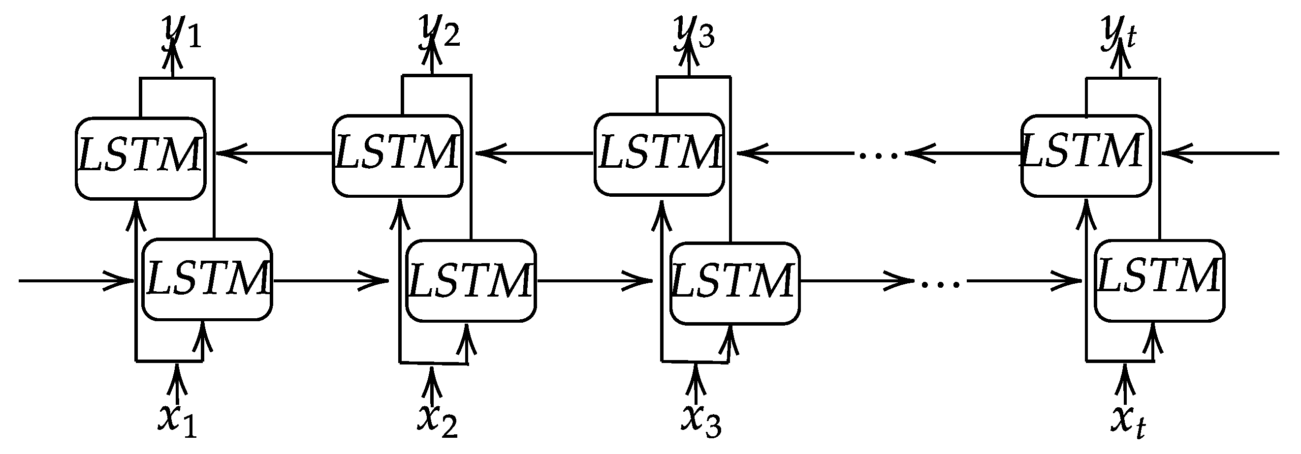
2.1. Recurrent Neural Network

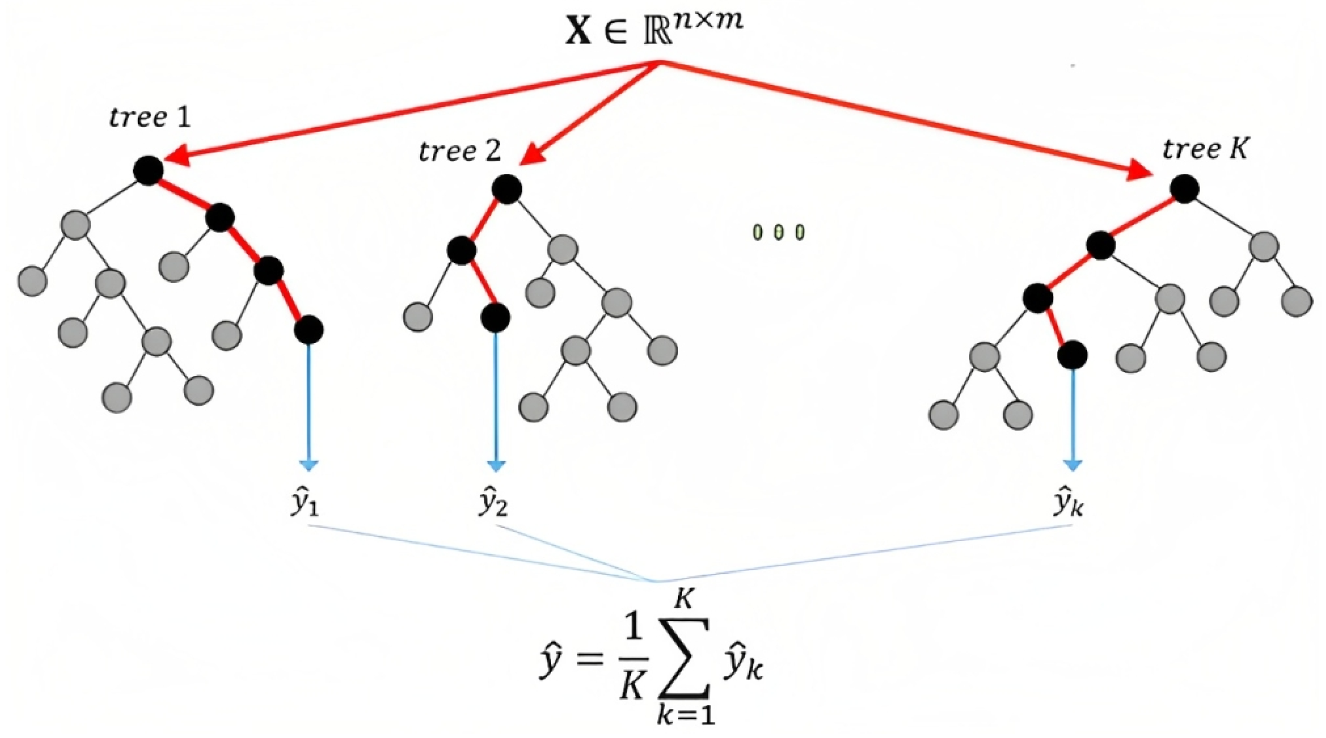
2.2. Random Forest

2.3. Support Vector Regression
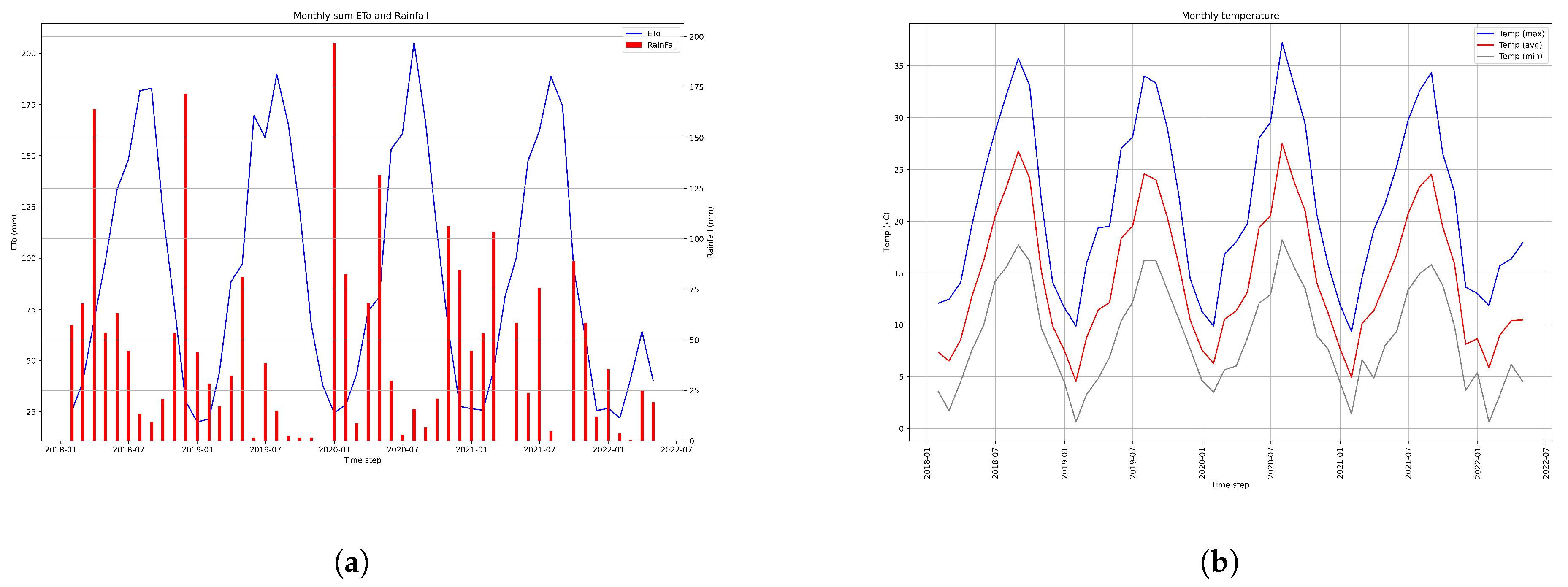
2.4. Datasets Used
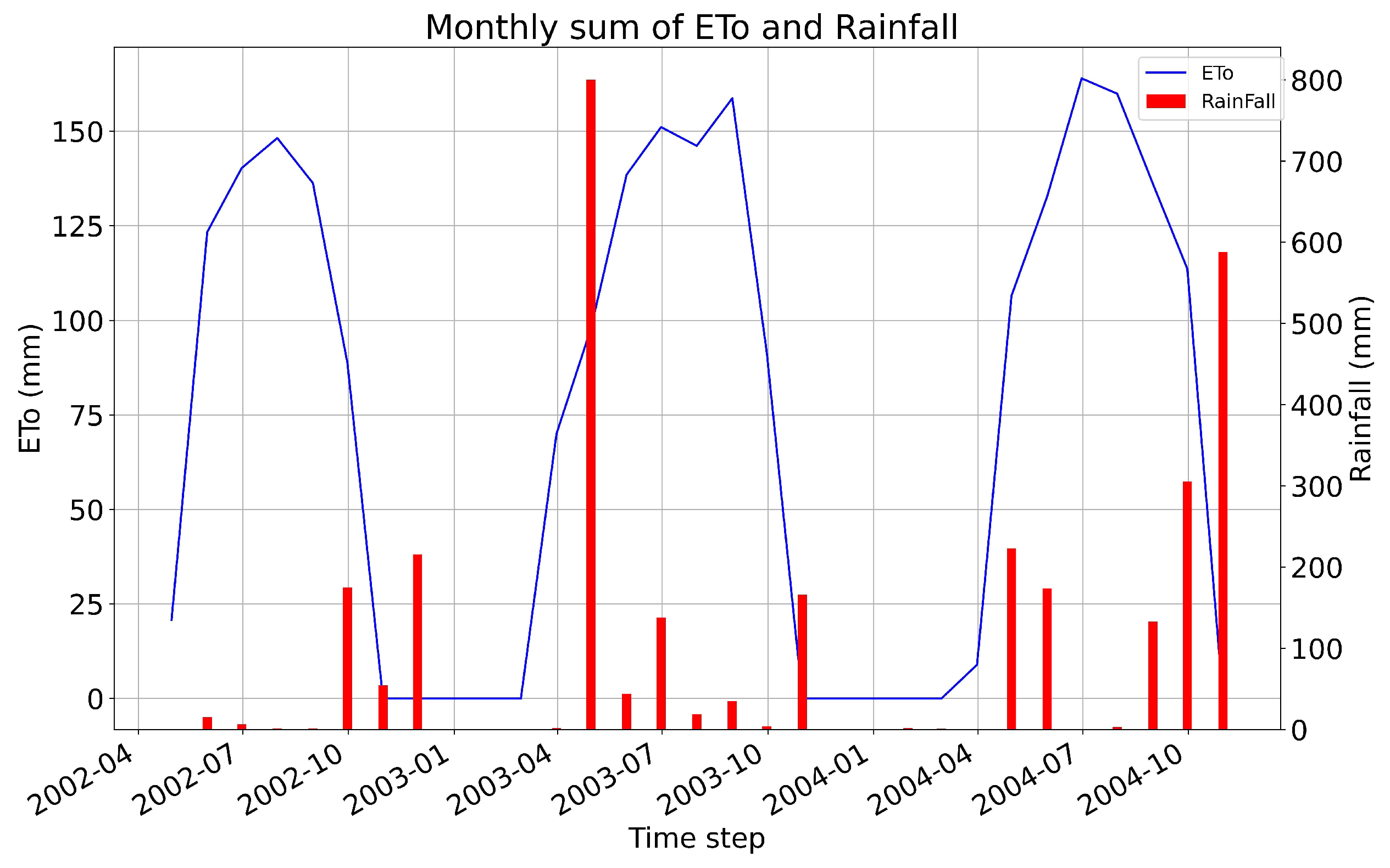
Test Dataset
2.5. Data Preprocessing
2.6. Training Configuration
Hyperparameters’ Selection
3. Results and Discussion
3.1. Training of the FTSW Prediction Model
3.2. Performance of the FTSW Prediction Model on Colinas do Douro Dataset
3.3. Performance of the FTSW Model on Quinta de Pancas Dataset
3.4. Comparison of FTSW Prediction Using the LSTM Model Performance with Other Models
4. Conclusions
Author Contributions
Funding
Institutional Review Board Statement
Informed Consent Statement
Data Availability Statement
Acknowledgments
Conflicts of Interest
References
- Clark, M.; Tilman, D. Comparative analysis of environmental impacts of agricultural production systems, agricultural input efficiency, and food choice. Environ. Res. Lett. 2017, 12, 064016. [Google Scholar] [CrossRef]
- Baiano, A. An Overview on Sustainability in the Wine Production Chain. Beverages 2021, 7, 15. [Google Scholar] [CrossRef]
- Rodrigo-Comino, J. Five decades of soil erosion research in “terroir”. The State-of-the-Art. Earth-Sci. Rev. 2018, 179, 436–447. [Google Scholar] [CrossRef]
- Sundmaeker, H.; Verdouw, C.N.; Wolfert, J.; Freire, L.P. Internet of Food and Farm 2020. In Digitising the Industry; Vermesan, O., Friess, P., Eds.; River Publishers: Gistrup, Denmark, 2016; pp. 129–150. [Google Scholar]
- Lohchab, V.; Kumar, M.; Suryan, G.; Gautam, V.; Das, R.K. A Review of IoT based Smart Farm Monitoring. In Proceedings of the 2018 Second International Conference on Inventive Communication and Computational Technologies (ICICCT), Coimbatore, India, 20–21 April 2018; pp. 1620–1625. [Google Scholar] [CrossRef]
- Nayyar, A.; Puri, V. Smart Farming: IoT Based Smart Sensors Agriculture Stick for Live Temperature and Moisture Monitoring Using Arduino, Cloud Computing & Solar Technology. In Proceedings of the The International Conference on Communication and Computing Systems (ICCCS-2016), Gurgaon, India, 9–11 September 2016; pp. 673–680. [Google Scholar] [CrossRef]
- De-Pablos-Heredero, C.; Montes-Botella, J.L.; García-Martínez, A. Sustainability in Smart Farms: Its Impact on Performance. Sustainability 2018, 10, 1713. [Google Scholar] [CrossRef]
- Said Mohamed, E.; Belal, A.; Kotb Abd-Elmabod, S.; El-Shirbeny, M.A.; Gad, A.; Zahran, M.B. Smart farming for improving agricultural management. Egypt. J. Remote Sens. Space Sci. 2021, 24, 971–981. [Google Scholar] [CrossRef]
- Verdouw, C.; Wolfert, S.; Tekinerdogan, B. Internet of Things in agriculture. CAB Rev. 2016, 11, 1–12. [Google Scholar] [CrossRef]
- Doshi, J.; Patel, T.; kumar Bharti, S. Smart Farming using IoT, a solution for optimally monitoring farming conditions. Procedia Comput. Sci. 2019, 160, 746–751, The 10th International Conference on Emerging Ubiquitous Systems and Pervasive Networks (EUSPN-2019) / The 9th International Conference on Current and Future Trends of Information and Communication Technologies in Healthcare (ICTH-2019) / AffiliatedWorkshops. [Google Scholar] [CrossRef]
- LeCun, Y.; Bengio, Y.; Hinton, G. Deep learning. Nature 2015, 521, 436–444. [Google Scholar] [CrossRef]
- Bengio, Y. Deep Learning of Representations for Unsupervised and Transfer Learning. In Proceedings of ICML Workshop on Unsupervised and Transfer Learning; Guyon, I., Dror, G., Lemaire, V., Taylor, G., Silver, D., Eds.; PMLR: Bellevue, WA, USA, 2012; Volume 27, Proceedings of Machine Learning Research; pp. 17–36. [Google Scholar]
- Kerkech, M.; Hafiane, A.; Canals, R. Vine disease detection in UAV multispectral images using optimized image registration and deep learning segmentation approach. Comput. Electron. Agric. 2020, 174, 105446. [Google Scholar] [CrossRef]
- Jiang, P.; Chen, Y.; Liu, B.; He, D.; Liang, C. Real-Time Detection of Apple Leaf Diseases Using Deep Learning Approach Based on Improved Convolutional Neural Networks. IEEE Access 2019, 7, 59069–59080. [Google Scholar] [CrossRef]
- Karthik, R.; Hariharan, M.; Anand, S.; Mathikshara, P.; Johnson, A.; Menaka, R. Attention embedded residual CNN for disease detection in tomato leaves. Appl. Soft Comput. 2020, 86, 105933. [Google Scholar]
- Silver, D.L.; Monga, T. In Vino Veritas: Estimating Vineyard Grape Yield from Images Using Deep Learning. In Advances in Artificial Intelligence; Meurs, M.J., Rudzicz, F., Eds.; Springer International Publishing: Cham, Switzerland, 2019; pp. 212–224. [Google Scholar]
- Aguiar, A.S.; Magalhães, S.A.; dos Santos, F.N.; Castro, L.; Pinho, T.; Valente, J.; Martins, R.; Boaventura-Cunha, J. Grape Bunch Detection at Different Growth Stages Using Deep Learning Quantized Models. Agronomy 2021, 11, 1890. [Google Scholar] [CrossRef]
- Ghiani, L.; Sassu, A.; Palumbo, F.; Mercenaro, L.; Gambella, F. In-Field Automatic Detection of Grape Bunches under a Totally Uncontrolled Environment. Sensors 2021, 21, 3908. [Google Scholar] [CrossRef]
- Assunção, E.; Gaspar, P.D.; Mesquita, R.; Simões, M.P.; Alibabaei, K.; Veiros, A.; Proença, H. Real-Time Weed Control Application Using a Jetson Nano Edge Device and a Spray Mechanism. Remote Sens. 2022, 14, 4217. [Google Scholar] [CrossRef]
- Wang, A.; Xu, Y.; Wei, X.; Cui, B. Semantic Segmentation of Crop and Weed using an Encoder-Decoder Network and Image Enhancement Method under Uncontrolled Outdoor Illumination. IEEE Access 2020, 8, 81724–81734. [Google Scholar] [CrossRef]
- Lottes, P.; Behley, J.; Milioto, A.; Stachniss, C. Fully Convolutional Networks With Sequential Information for Robust Crop and Weed Detection in Precision Farming. IEEE Robot. Autom. Lett. 2018, 3, 2870–2877. [Google Scholar] [CrossRef]
- Li, C.; Zhang, Y.; Ren, X. Modeling Hourly Soil Temperature Using Deep BiLSTM Neural Network. Algorithms 2020, 13, 173. [Google Scholar] [CrossRef]
- Yu, F.; Hao, H.; Li, Q. An Ensemble 3D Convolutional Neural Network for Spatiotemporal Soil Temperature Forecasting. Sustainability 2021, 13, 9174. [Google Scholar] [CrossRef]
- Saggi, M.K.; Jain, S. Reference evapotranspiration estimation and modeling of the Punjab Northern India using deep learning. Comput. Electron. Agric. 2019, 156, 387–398. [Google Scholar] [CrossRef]
- Loggenberg, K.; Strever, A.; Greyling, B.; Poona, N. Modelling Water Stress in a Shiraz Vineyard Using Hyperspectral Imaging and Machine Learning. Remote Sens. 2018, 10, 202. [Google Scholar] [CrossRef]
- Acharya, U.; Daigh, A.L.M.; Oduor, P.G. Machine Learning for Predicting Field Soil Moisture Using Soil, Crop, and Nearby Weather Station Data in the Red River Valley of the North. Soil Syst. 2021, 5, 57. [Google Scholar] [CrossRef]
- Fang, K.; Shen, C.; Kifer, D.; Yang, X. Prolongation of SMAP to Spatiotemporally Seamless Coverage of Continental U.S. Using a Deep Learning Neural Network. Geophys. Res. Lett. 2017, 44, 11030–11039. [Google Scholar] [CrossRef]
- Ek, M.B.; Mitchell, K.E.; Lin, Y.; Rogers, E.; Grunmann, P.; Koren, V.; Gayno, G.; Tarpley, J.D. Implementation of Noah land surface model advances in the National Centers for Environmental Prediction operational mesoscale Eta model. J. Geophys. Res. Atmos. 2003, 108, 1–12. [Google Scholar] [CrossRef]
- Paul, S.; Singh, S. Soil Moisture Prediction Using Machine Learning Techniques. In Proceedings of the 3rd International Conference on Computational Intelligence and Intelligent Systems, CIIS 2020, Tokyo, Japan, 13–15 November 2020; Association for Computing Machinery: New York, NY, USA, 2020; pp. 1–7. [Google Scholar] [CrossRef]
- Adeyemi, O.; Grove, I.; Peets, S.; Domun, Y.; Norton, T. Dynamic Neural Network Modelling of Soil Moisture Content for Predictive Irrigation Scheduling. Sensors 2018, 18, 3408. [Google Scholar] [CrossRef]
- Hajjar, C.S.; Hajjar, C.; Esta, M.; Chamoun, Y.G. Machine learning methods for soil moisture prediction in vineyards using digital images. E3S Web Conf. 2020, 167, 02004. [Google Scholar] [CrossRef]
- Zhang, J.; Zhu, Y.; Zhang, X.; Ye, M.; Yang, J. Developing a Long Short-Term Memory (LSTM) based model for predicting water table depth in agricultural areas. J. Hydrol. 2018, 561, 918–929. [Google Scholar] [CrossRef]
- Chen, M.; Cui, Y.; Wang, X.; Xie, H.; Liu, F.; Luo, T.; Zheng, S.; Luo, Y. A reinforcement learning approach to irrigation decision-making for rice using weather forecasts. Agric. Water Manag. 2021, 250, 106838. [Google Scholar] [CrossRef]
- Alibabaei, K.; Gaspar, P.D.; Assunção, E.; Alirezazadeh, S.; Lima, T.M. Irrigation optimization with a deep reinforcement learning model: Case study on a site in Portugal. Agric. Water Manag. 2022, 263, 107480. [Google Scholar] [CrossRef]
- Pellegrino, A.; Lebon, E.; Voltz, M.; Wery, J. Relationships between plant and soil water status in vine (Vitis vinifera L.). Plant Soil 2005, 266, 129–142. [Google Scholar] [CrossRef]
- Rallo, G.; Provenzano, G. Modelling eco-physiological response of table olive trees (Olea europaea L.) to soil water deficit conditions. Agric. Water Manag. 2013, 120, 79–88, Soil and Irrigation Sustainability Practices. [Google Scholar] [CrossRef]
- Lebon, E.; Dumas, V.; Pieri, P.; Schultz, H.R. Modelling the seasonal dynamics of the soil water balance of vineyards. Funct. Plant Biol. 2003, 30, 699. [Google Scholar] [CrossRef]
- Lopes, C.M.; Santos, T.P.; Monteiro, A.; Rodrigues, M.L.; Costa, J.M.; Chaves, M.M. Combining cover cropping with deficit irrigation in a Mediterranean low vigor vineyard. Sci. Hortic. 2011, 129, 603–612. [Google Scholar] [CrossRef]
- Phogat, V.; Petrie, P.R.; Collins, C.; Bonada, M. Plant available water capacity of soils at regional scale: Analysis of fixed and dynamic field capacity. Pedosphere 2022, in press. [Google Scholar] [CrossRef]
- Ramos, M.; Casasnovas, J.M. Soil water variability and its influence on transpirable soil water fraction with two grape varieties under different rainfall regimes. Agric. Ecosyst. Environ. 2014, 185, 253–262. [Google Scholar] [CrossRef]
- Valdés-Gómez, H.; Celette, F.; García de Cortázar-Atauri, I.n.; Jara-Rojas, F.; Ortega-Farías, S.; Gary, C. Modelling soil water content and grapevine growth and development with the stics crop-soil model under two different water management strategies. Oeno One 2009, 43, 13–28. [Google Scholar] [CrossRef]
- Marhon, S.A.; Cameron, C.J.F.; Kremer, S.C. Recurrent Neural Networks. In Handbook on Neural Information Processing; Bianchini, M., Maggini, M., Jain, L.C., Eds.; Springer: Berlin/Heidelberg, Germany, 2013; pp. 29–65. [Google Scholar] [CrossRef]
- Hochreiter, S.; Schmidhuber, J. Long Short-Term Memory. Neural Comput. 1997, 9, 1735–1780. [Google Scholar] [CrossRef]
- Alibabaei, K.; Gaspar, P.D.; Lima, T.M. Modeling Soil Water Content and Reference Evapotranspiration from Climate Data Using Deep Learning Method. Appl. Sci. 2021, 11, 5029. [Google Scholar] [CrossRef]
- Breiman, L. Random Forests. Mach. Learn. 2001, 45, 5–32. [Google Scholar] [CrossRef]
- Dang, V.H.; Hoang, N.D.; Nguyen, L.M.D.; Bui, D.T.; Samui, P. A Novel GIS-Based Random Forest Machine Algorithm for the Spatial Prediction of Shallow Landslide Susceptibility. Forests 2020, 11, 118. [Google Scholar] [CrossRef]
- Allen, R.G.; Pereira, L.S.; Raes, D.; Smith, M. Crop Evapotranspiration—Guidelines for Computing Crop Water Requirements FAO Irrigation and Drainage Paper 56; FAO—Food and Agriculture Organization of the United Nations: Rome, Italy, 1998. [Google Scholar]
- Sinclair, T.; Ludlow, M. Influence of Soil Water Supply on the Plant Water Balance of Four Tropical Grain Legumes. Funct. Plant Biol. 1986, 13, 329. [Google Scholar] [CrossRef]
- Monteiro, A.; Lopes, C.M. Influence of cover crop on water use and performance of vineyard in Mediterranean Portugal. Agric. Ecosyst. Environ. 2007, 121, 336–342. [Google Scholar] [CrossRef]
- Hargreaves, G.H.; Samani, Z.A. Reference Crop Evapotranspiration from Temperature. Appl. Eng. Agric. 1985, 1, 96–99. [Google Scholar] [CrossRef]
- Rodrigues, G.C.; Braga, R.P. Estimation of Reference Evapotranspiration during the Irrigation Season Using Nine Temperature-Based Methods in a Hot-Summer Mediterranean Climate. Agriculture 2021, 11, 124. [Google Scholar] [CrossRef]
- Schmidhuber, J. Deep learning in neural networks: An overview. Neural Netw. 2015, 61, 85–117. [Google Scholar] [CrossRef]
- Hsu, C.W.; Chang, C.C.; Lin, C.J. A Practical Guide to Support Vector Classification; Technical Report; Department of Computer Science, National Taiwan University: Taibei, Taiwan, 2003. [Google Scholar]
- Bergstra, J.; Bengio, Y. Random Search for Hyper-Parameter Optimization. J. Mach. Learn. Res. 2012, 13, 281–305. [Google Scholar]
- Bergstra, J.; Bardenet, R.; Bengio, Y.; Kégl, B. Algorithms for Hyper-Parameter Optimization. In Proceedings of the 24th International Conference on Neural Information Processing Systems, NIPS’11, Granada, Spain, 12–15 December 2011; Curran Associates Inc.: Red Hook, NY, USA, 2011; pp. 2546–2554. [Google Scholar]
- Molnar, C. A Guide for Making Black Box Models Explainable. In Interpretable Machine Learning, 2nd ed.; Lulu Press, Inc.: Morrisville, NC, USA, 2022. [Google Scholar]
- Wei, P.; Lu, Z.; Song, J. Variable importance analysis: A comprehensive review. Reliab. Eng. Syst. Saf. 2015, 142, 399–432. [Google Scholar] [CrossRef]
- James, G.; Witten, D.; Hastie, T.; Tibshirani, R. An Introduction to Statistical Learning: With Applications in R; Springer Publishing Company, Incorporated: Berlin/Heidelberg, Germany, 2014. [Google Scholar]
- Prechelt, L. Early Stopping—But When? In Neural Networks: Tricks of the Trade: Second Edition; Montavon, G., Orr, G.B., Müller, K.R., Eds.; Springer: Berlin/Heidelberg, Germany, 2012; pp. 53–67. [Google Scholar]
- Brocca, L.; Morbidelli, R.; Melone, F.; Moramarco, T. Soil moisture spatial variability in experimental areas of central Italy. J. Hydrol. 2007, 333, 356–373. [Google Scholar] [CrossRef]
- Cosh, M.H.; Stedinger, J.R.; Brutsaert, W. Variability of surface soil moisture at the watershed scale. Water Resour. Res. 2004, 40, 1–9. [Google Scholar] [CrossRef]


| Variables | Year | ||||||||
|---|---|---|---|---|---|---|---|---|---|
| 2018 | 2019 | 2020 | 2021 | ||||||
| Mean | Std | Mean | Std | Mean | Std | Mean | Std | ||
| Temp (C) | Avg | 14.97 | 7.59 | 14.86 | 7.05 | 15.58 | 7.16 | 14.87 | 6.79 |
| Max | 21.79 | 9.38 | 22.09 | 8.84 | 22.56 | 9.24 | 21.96 | 8.65 | |
| Min | 9.43 | 5.9 | 8.95 | 5.64 | 9.8 | 5.35 | 8.96 | 5.54 | |
| RH(%) | Avg | 64.72 | 17.88 | 63.14 | 17.43 | 65.08 | 19.03 | 63.97 | 16.15 |
| Max | 85.05 | 12.06 | 84.6 | 11.86 | 85.83 | 13.75 | 85.57 | 10.18 | |
| Min | 41.2 | 20.34 | 38.73 | 20.77 | 41.32 | 21.59 | 39.82 | 19.32 | |
| WS (m/s) | Avg | 1.63 | 1.16 | 1.64 | 1.23 | 1.52 | 1.1 | 1.43 | 1.06 |
| Max | 4.3 | 2.21 | 4.14 | 2.17 | 3.98 | 2.11 | 3.8 | 2.04 | |
| VPD (kPa) | Avg | 0.9 | 0.85 | 0.89 | 0.73 | 0.93 | 0.9 | 0.86 | 0.72 |
| Min | 0.23 | 0.27 | 0.21 | 0.22 | 0.23 | 0.29 | 0.2 | 0.2 | |
| Rainfall (mm) | Sum | 2.1 | 5.2 | 1.14 | 5.22 | 1.65 | 5.11 | 1.41 | 4.23 |
| ETo (mm) | Daily | 3.1 | 2.03 | 3.26 | 2.09 | 3.13 | 2.09 | 3.11 | 2.03 |
| Variables | Temporal | Year | ||||||||
|---|---|---|---|---|---|---|---|---|---|---|
| Resolution | 2018 | 2019 | 2020 | 2021 | ||||||
| Max | Min | Max | Min | Max | Min | Max | Min | |||
| VSM (%) | 20 cm | Daily | 31.56 | 10.85 | 31.82 | 11.16 | 32.52 | 10.86 | 32.40 | 11.18 |
| 40 cm | Daily | 28.96 | 10.89 | 28.06 | 10.64 | 29.75 | 10.62 | 29.83 | 12.01 | |
| 60 cm | Daily | 31.68 | 11.05 | 27.39 | 10.96 | 31.93 | 11.24 | 29.99 | 12.27 | |
| 80 cm | Daily | 33.43 | 12.56 | 27.53 | 12.56 | 33.29 | 12.79 | 28.29 | 13.43 | |
| VSM (mm) | summed | Daily | 209.11 | 81.15 | 190.04 | 84.52 | 217 | 79.33 | 202.19 | 85.66 |
| Model | Batch Size | Dropout Size | Learning Rate | Decay | No. of Units |
|---|---|---|---|---|---|
| FTSW prediction model | 40 | 0.09313 | 0.003968 | 0.003456 | 158 |
| Input Variables | Input Length (Look-back) | Output Length |
|---|---|---|
| Month, ETo, RH (avg), rainfall | 3, 5,7 | 1 |
| Month, ETo, rainfall RH (avg), VPD (min) | 3, 5, 7 | 1 |
| Month, ETo, rainfall, RH (avg), VPD (min), irr | 3, 5, 7 | 3, 5, 7 |
| Input Variables | Look-Back (Days) | Colinas do Douro | |||
|---|---|---|---|---|---|
| Validation Set | Test Set | ||||
| -Score | RMSE (Normalized) | -Score | RMSE | ||
| Month, ETo, RH (avg), rainfall, | 3 | 0.75 | 0.6 | 0.75 | 16.6 |
| 5 | 0.81 | 0.56 | 0.81 | 14.4 | |
| 7 | 0.87 | 0.54 | 0.90 | 10.75 | |
| Month, ETo, rainfall RH (avg), VPD (min) | 3 | 0.77 | 0.50 | 0.79 | 15.39 |
| 5 | 0.83 | 0.53 | 0.85 | 12.78 | |
| 7 | 0.92 | 0.41 | 0.93 | 8.98 | |
| Month, ETo, rainfall, RH (avg), VPD (min), irr | 3 | 0.75 | 0.51 | 0.79 | 15.34 |
| 5 | 0.87 | 0.46 | 0.86 | 12.53 | |
| 7 | 0.96 | 0.31 | 0.94 | 8.03 | |
| Input Variables | Look-Back | Output | Colinas do Douro | |||
|---|---|---|---|---|---|---|
| Validation Set | Test Set | |||||
| -Score | RMSE | -Score | RMSE | |||
| Month, ETo,RH (avg), rainfall, irr | 3 | 3 | 0.61 | 0.60 | 0.58 | 21.37 |
| 5 | 5 | 0.80 | 0.46 | 0.74 | 16.77 | |
| 7 | 7 | 0.32 | 0.89 | 0.90 | 10.35 | |
| Month, ETo, RH (avg), rainfall, irr VPD (min) | 3 | 3 | 0.69 | 0.57 | 0.64 | 19.68 |
| 5 | 5 | 0.44 | 0.80 | 0.81 | 14.54 | |
| 7 | 7 | 0.31 | 0.88 | 0.92 | 9.19 | |
| Location | RMSE | -Score |
|---|---|---|
| Quinta de pancas | 10.22 | 0.87 |
| Colinas do Douro | 8.43 | 0.93 |
| SVR | RF | ||
|---|---|---|---|
| Hparam | Value | Hparam | Value |
| C | 1.83 | n_estimators | 118 |
| kernel | RBF | bootstrap | False |
| bootstrap | False | ||
| gamma | scale | max depth | 110 |
| epsilon | 0.26 | max_features | Sqrt |
| - | - | Min samples leaf | 2 |
| - | - | Min samples split | 2 |
| Model | Quinta de Pancas | Colinas do Douro | ||
|---|---|---|---|---|
| RMSE | -Score | RMSE | -Score | |
| BiLSTM | 10.36 | 0.87 | 8.3 | 0.93 |
| RF | 16.8 | 0.67 | 12.88 | 0.85 |
| SVR | 19.43 | 0.58 | 14.15 | 0.82 |
| LR | 22.5 | 0.43 | 18.68 | 0.69 |
Disclaimer/Publisher’s Note: The statements, opinions and data contained in all publications are solely those of the individual author(s) and contributor(s) and not of MDPI and/or the editor(s). MDPI and/or the editor(s) disclaim responsibility for any injury to people or property resulting from any ideas, methods, instructions or products referred to in the content. |
© 2023 by the authors. Licensee MDPI, Basel, Switzerland. This article is an open access article distributed under the terms and conditions of the Creative Commons Attribution (CC BY) license (https://creativecommons.org/licenses/by/4.0/).
Share and Cite
Alibabaei, K.; Gaspar, P.D.; Campos, R.M.; Rodrigues, G.C.; Lopes, C.M. Evaluation of a Deep Learning Approach for Predicting the Fraction of Transpirable Soil Water in Vineyards. Appl. Sci. 2023, 13, 2815. https://doi.org/10.3390/app13052815
Alibabaei K, Gaspar PD, Campos RM, Rodrigues GC, Lopes CM. Evaluation of a Deep Learning Approach for Predicting the Fraction of Transpirable Soil Water in Vineyards. Applied Sciences. 2023; 13(5):2815. https://doi.org/10.3390/app13052815
Chicago/Turabian StyleAlibabaei, Khadijeh, Pedro D. Gaspar, Rebeca M. Campos, Gonçalo C. Rodrigues, and Carlos M. Lopes. 2023. "Evaluation of a Deep Learning Approach for Predicting the Fraction of Transpirable Soil Water in Vineyards" Applied Sciences 13, no. 5: 2815. https://doi.org/10.3390/app13052815
APA StyleAlibabaei, K., Gaspar, P. D., Campos, R. M., Rodrigues, G. C., & Lopes, C. M. (2023). Evaluation of a Deep Learning Approach for Predicting the Fraction of Transpirable Soil Water in Vineyards. Applied Sciences, 13(5), 2815. https://doi.org/10.3390/app13052815