Classification of the Central Effects of Transcutaneous Electroacupuncture Stimulation (TEAS) at Different Frequencies: A Deep Learning Approach Using Wavelet Packet Decomposition with an Entropy Estimator

Abstract

The field of signal processing using machine and deep learning algorithms has undergone significant growth in the last few years, with a wide scope of practical applications for electroencephalography (EEG). Transcutaneous electroacupuncture stimulation (TEAS) is a well-established variant of the traditional method of acupuncture that is also receiving increasing research attention. This paper presents the results of using deep learning algorithms on EEG data to investigate the effects on the brain of different frequencies of TEAS when applied to the hands in 66 participants, before, during and immediately after 20 min of stimulation. Wavelet packet decomposition (WPD) and a hybrid Convolutional Neural Network Long Short-Term Memory (CNN-LSTM) model were used to examine the central effects of this peripheral stimulation. The classification results were analysed using confusion matrices, with kappa as a metric. Contrary to expectation, the greatest differences in EEG from baseline occurred during TEAS at 80 pulses per second (pps) or in the ‘sham’ (160 pps, zero amplitude), while the smallest differences occurred during 2.5 or 10 pps stimulation (mean kappa 0.414). The mean and CV for kappa were considerably higher for the CNN-LSTM than for the Multilayer Perceptron Neural Network (MLP-NN) model. As far as we are aware, from the published literature, no prior artificial intelligence (AI) research appears to have been conducted into the effects on EEG of different frequencies of electroacupuncture-type stimulation (whether EA or TEAS). This ground-breaking study thus offers a significant contribution to the literature. However, as with all (unsupervised) DL methods, a particular challenge is that the results are not easy to interpret, due to the complexity of the algorithms and the lack of a clear understanding of the underlying mechanisms. There is therefore scope for further research that explores the effects of the frequency of TEAS on EEG using AI methods, with the most obvious place to start being a hybrid CNN-LSTM model. This would allow for better extraction of information to understand the central effects of peripheral stimulation.

1. Introduction

‘Signals due to rhythmic stimulation... appear to reach parts of the central nervous system which are inaccessible to impulses set up by non-rhythmic stimuli, however intense’ (William Grey Walter) [1].

Transcutaneous electroacupuncture stimulation (TEAS), a non-invasive variant of the ancient method of acupuncture that has been used since the 1990s. It is increasingly used in clinical practice, most commonly for pain management and in a range of musculoskeletal presentations, predominantly in China [2]. TEAS has also been shown, for example, to be effective in the treatment of stroke [3], post-operative nausea and vomiting [4], and for improving symptoms of insomnia and anxiety in opioid use disorder [5].

In contrast to classical acupuncture, TEAS does not involve any puncture of the skin or the use of any needles. It is therefore potentially advantageous for any patient who has a fear of needles (so-called needle phobia) or for whom skin puncture might be considered an unacceptable clinical risk. Ulett et al. (1998) [6] identified that the effects of classic electroacupuncture (via needles) are stronger and more profound than those achieved with manual acupuncture (employing a needle but with no electrical stimulation). Furthermore, electroacupuncture with surface electrodes was demonstrated to be as effective as needle-based electroacupuncture.

In functional magnetic resonance imaging (fMRI) studies, electroacupuncture has been shown to generate more widespread cerebral and sub-cortical changes than manual acupuncture [7,8], and thus, the use of TEAS may have real physiological advantages over classical manual acupuncture.

The safety concerns associated with acupuncture [9], although largely theoretical, can be ameliorated through the use of a surface electrode stimulating system (i.e., TEAS).

The potential for home-based, patient-delivered acupuncture may have significant advantages (reduced cost, and a lower clinical burden for both the patient and the clinician). TEAS makes a home-based delivery system a realistic proposition [10].

Based on a series of several small pilot studies conducted between 2011 and 2015, in 2016–2017, a larger study was conducted (N = 66) with the same primary objective, namely, to ascertain if electroacupuncture stimulation—whether applied using needles or transcutaneously—has frequency-specific effects on electroencephalography (EEG) and other physiological signals. In the current study, we also expect to see differences in the effects depending on participant age, gender, personality and mood, as well as in the subjectively reported intensity of stimulation. Our objective in this first neuroimaging report is to determine if there is a difference between the EEG at baseline (before stimulation), during transcutaneous electroacupuncture stimulation (TEAS) and after stimulation, and whether these differences vary with stimulation frequency.

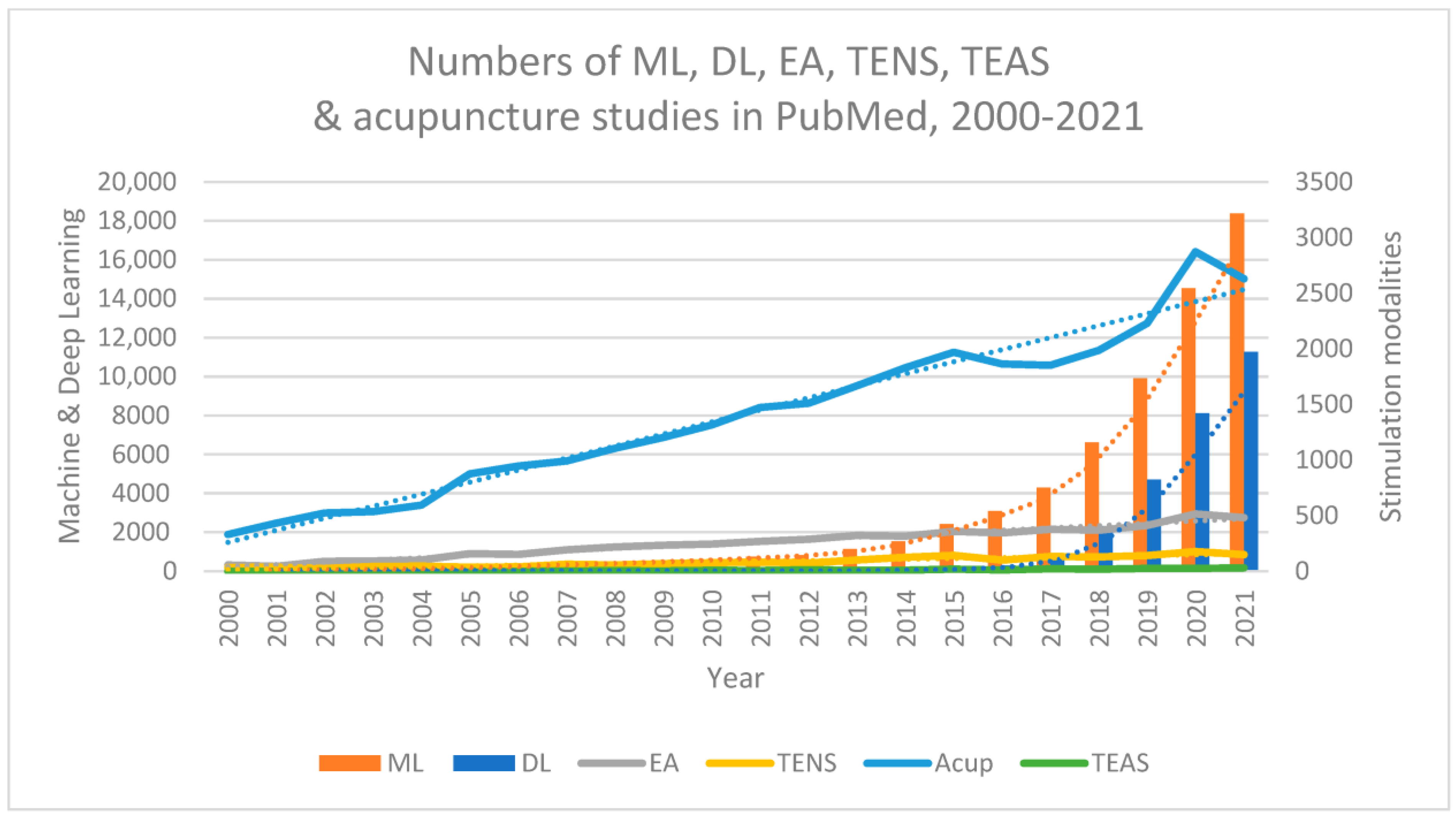
To try to answer our research question, we decided to use deep learning (DL), a twenty-first-century method of data analysis that has evolved from machine learning (ML). The application of both of these artificial intelligence (AI) methods of data analysis has been increasing exponentially over the past decade, whereas research on acupuncture-related stimulation methods has grown steadily and more or less linearly over the same period (Figure 1).

1.1. A Brief Overview of AI: Machine Learning (ML) and Deep Learning (DL) in EEG Analysis

As an experiment in learning, a series of nested literature reviews were conducted on or around the 5 December 2021. In the first of these, 2118 papers were located on PubMed.gov by using the search string ‘EEG AND (“machine learning” OR “deep learning”)’. Of the 2118 hits, almost a quarter (473, or 22.3%) included the terms ‘epilepsy OR seizure*’. 138 (6.5%) of this subset of papers were reviewed, and 47 of these (34.1%, or more than a third) were on epilepsy or seizures.

In contrast, only one of the 2118 papers found was on acupuncture [11], and none were on transcutaneous electrical nerve stimulation (TENS), although one was located that mentioned transcutaneous vagal stimulation [12]. Widening the search strategy to locate acupuncture or TENS studies using ML or DL methods, but not necessarily applying them primarily to EEG, a further useful review paper on acupuncture, ML and neuroimaging (including EEG) was located on PubMed [13]. Only one paper on electroacupuncture (EA) and ML was located [14], but ML was used here as a method of predicting clinical outcomes, not in the analysis of physiological signals. For bibliometric comparison, comparable searches were also made using SCOPUS, Elsevier’s citation database [15] and the resources of CNKI (China National Knowledge Infrastructure, 中国知网) (https://cnki.net/) (accessed on 17 February 2023), although the results of the latter appeared somewhat variable, depending on when the searches were conducted.

Based on the literature located using PubMed and other online sources, a brief overview of ML and DL methods used for EEG data analysis is provided in the online Supplementary Materials, Section SM1. It is not exhaustive and is intended simply to provide enough background information for those unfamiliar with the language of AI to understand the methods and results of our analysis.

1.2. Literature Review and Resulting Proposed Strategy

Combinations and comparisons of ML and DL algorithms were located in PubMed-indexed papers using the search terms ‘EEG AND [ML A] AND [DL A],’ where [ML A] and [DL A] are the standard acronyms for the DL and ML algorithms, respectively. The exceptions were PCA (Principal Component Analysis) and RF (Random Forest), which were searched using their full names. The results of the searches conducted on 5 December 2021 are shown in

Table 1. Combinations and comparisons of ML and DL algorithms (A) located in PubMed-indexed papers using the search terms ‘EEG AND [ML A] AND [DL A].’ Combination and comparison counts were taken from study abstracts. Where this classification was not obvious, counts are included in the ‘Other/Unclear’ column. Abbreviations used: CNN: Convolutional Neural Network; DNN: Deep Neural Network; LDA: Linear Discriminant Analysis; LR: Logistic Regression; LSTM: Long Short-Term Memory; PCA: Principal Component Analysis; RNN: Recurrent Neural Network; SVM: Support Vector Machine. These terms are explained in more detail in the online Supplementary Materials (SM1).

DL Algorithm	ML Algorithm	Counts (All)	Combinations	Comparisons	Other/Unclear
CNN	SVM	29	9	20	0
	RF	17	4	10	3
	LDA	7	0	0	0
	LR	5	1	0	1
	Clustering	10	3	0	6
	PCA	1	0	0	0
Sum		69	17	30	10
LSTM	SVM	15	5	10	0
	RF	7	1	6	0
	LDA	3	1	2	0
	LR	0	0	0	0
	Clustering	2	n/a	n/a	2
	PCA	2	1	1	0
Sum		29	8	19	2
RNN	SVM	6	1	3	2
	RF	5	1	3	1
	LDA	1	0	1	0
	LR	0	0	0	0
	Clustering	1	n/a	n/a	1
	PCA	0	0	0	0
Sum		14	2	7	4
DNN	SVM	6	4	2	0
	RF	2	1	1	0
	LDA	2	1	1	0
	LR	0	0	0	0
	Clustering	2	2	0	0
	PCA	0	0	0	0
Sum		11	8	4	0
	SVM	56	19	35	2
	RF	31	7	20	4
	LDA	13	2	11	0
	LR	5	1	3	1
	Clustering	15	5	1	9
	PCA	3	1	2	0

Note: Clustering (or obvious synonyms) did not appear in some papers located in PubMed when using the search term ‘cluster*,’ while in some papers that did include clustering, it did not appear to be used as an ML method. For Logistic Regression (LR), one study did not provide results for either the combination or comparison of methods [16] NB: Not all (non-feature-based) DL methods outperformed (feature-based) ML methods (see some of the Support Vector Machine vs. Convolutional Neural Network (SVM vs. CNN) studies, for example).

.

Table 2. Results of PubMed searches for combinations or comparisons of two DL algorithms (for abbreviations, see caption of previous table).

DL Algorithm	ML Algorithm	Counts (All)	Combinations	Comparisons/Other
CNN	[CNN]
	LSTM	44	14	30
	RNN	13	4	9
	DNN	11	0	11
Sum		68	18	50
LSTM	CNN	44	2	42
	[LSTM]
	RNN	17	4	13
	DNN	7	0	7
Sum		68	6	62
RNN	CNN	13	0	13
	LSTM	17	1	16
	[RNN]
	DNN	1	1	0
Sum		31	2	29
DNN	CNN
	LSTM	11	0	11
	RNN	7	0	7
	[DNN]	1	1	0
Sum		19	1	18

shows the results of the PubMed searches for combinations or comparisons of the two DL algorithms, carried out on 5 December 2021.

CNN-LSTM models are thus relatively common hybrids and are more common than LSTM-CNN, the inverse combination. CNN-RNN and LSTM-RNN are the next most common hybrid models. This was confirmed for DL algorithms in general (i.e., not restricted to EEG studies), using Google Scholar instead of PubMed (the abbreviations are defined in the caption of Table 1, and explained in the online Supplementary Materials, SM1). CNN-LSTM thus appears to be an appropriate hybrid model for the current study. For those unfamiliar with CNN and LSTM, a description is provided in the online Supplementary Materials (SM2.1 and SM2.2).

1.3. Literature Review of AI, Acupuncture and EEG

A brief review was conducted of studies indexed in three major online databases—PubMed, SCOPUS and CNKI—on machine learning (ML), Support Vector Machines (SVM), deep learning (DL) or Convolutional Neural Networks (CNN) and electroencephalography (EEG), acupuncture (Acup) or electroacupuncture (EA). SVM and CNN were selected as frequently used exemplars of ML and DL, respectively. The results are shown in

Table 3. Numbers of studies located on 5 December 2021 in PubMed, SCOPUS and CNKI on machine learning (ML), Support Vector Machines (SVM), deep learning (DL) or Convolutional Neural Networks (CNN) and electroencephalography (EEG), acupuncture (Ac) or electroacupuncture (EA).

	PubMed				SCOPUS				CNKI
	ALL	EEG	Ac	EA	ALL	EEG	Ac	EA	ALL	EEG	Ac	EA
Machine learning 机器学习	60,085	1711	30	1	315,567	3957	38	3	290,855	1516	34	2
Support Vector Machine 支持向量机	18,367	1277	15	0	145,475	4617	37	2	114,018	583	14	2
Deep learning 深度学习	25,456	627	5	0	165,435	1982	2	1	213,990	786	28	7
Convolutional Neural Network 卷积神经网络	13,580	480	4	0	102,937	1659	5	2	125,390	676	8	0
Acupuncture 针刺	34,611	309			50,417	288			194,603	463
Electroacupuncture 电针	6350	69			9267	62			44,088	122

.

The percentage of all ML studies that mention SVM was thus lowest in PubMed (30.57%) and highest in SCOPUS (46.10%). Similarly, the percentage of all DL studies that mention CNN was lowest in PubMed (53.35%) and highest in SCOPUS (62.22%). In both PubMed and SCOPUS, a greater percentage of EEG studies mentioned SVM than CNN, but this was reversed in CNKI, suggesting geographical bias.

1.3.1. Neuroimaging and the Neurochemical Model of EA, TEAS and Acupuncture

The effects of EA, TEAS (and, indeed, acupuncture) are usually explained using neurochemical models, in which different regions of the brain play key roles [17,18]. In particular, stimulation at low, medium and high frequencies, or low or high amplitudes, may activate different pathways in the spinal cord and brain [18]. In brief, low-frequency stimulation (at 2–4 Hz) activates both large- and small-diameter afferents, and thus, has both segmental and supraspinal effects, with the release of enkephalin and beta-endorphin in the brain (less so in the spinal cord). These central effects may mean that any resulting analgesia has a slow onset and outlasts the stimulation itself. In contrast, high-frequency stimulation (at 50–200 Hz) activates predominantly the large-diameter afferents, so that the effects are segmental (associated with the release of dynorphin in the spinal cord), not supraspinal. Analgesia thus has a rapid onset but does not last long. Stimulation frequencies of 10–20 Hz may activate both mechanisms [19]. Numerous functional magnetic imaging (fMRI) studies have been conducted to explore these connections, but far less research has investigated the effects of acupuncture, EA or TEAS on EEG (315, 69 and 2 studies are currently indexed in PubMed, respectively), despite the advantages of EEG over other forms of neuroimaging, such as fMRI and magnetoencephalography (MEG) in terms of cost, portability and/or temporal resolution and usefulness for frequency analysis.

1.3.2. EEG Studies on Acupuncture and Related Modalities

Using the search string ‘EEG AND (acupuncture OR transcutaneous) NOT (“vagal stimulation” OR “vagus nerve stimulation”),’ about 500 studies were identified in PubMed. Of these, around 147, published between 1986 and 2022, were easily retrieved and could be examined in depth. Here, we consider those on steady-state EEG rather than evoked potentials. Of these, 56 (around 38%) were from China, 15 from Korea, 13 from the US, 11 from Japan and 10 from Taiwan. Other countries were represented by fewer than 10 studies each. Of the Chinese studies, 25 (more than 44%), or almost half, were from Hebei University of Technology (Tianjin University).

Most of these EEG studies were on manual acupuncture, and it should be remembered that ‘TEAS is different from insertive electroacupuncture in many ways, and the results from these studies may not apply to acupuncture’ [20]. In the acupuncture-related studies, the points most commonly used—as noted in a 2018 systematic review of 19 EEG acupuncture studies [21]—were ST36 (zusanli, 足三里, Zúsānlǐ), on the leg below the knee and lateral to the anterior crest of the tibia; LI4 (hegu, 合谷, Hégǔ), located in the area covered by the superficial branch of the radial nerve, and close to the radial artery or first dorsal metacarpal artery, i.e., on the back of the hand between the first and second metacarpals; and P6 (neiguan, 内关, Nèiguān), on the anterior surface of the forearm, proximal to the wrist crease between the palmaris longus and flexor carpi radialis tendons.

Methods of analysing changes in EEG were varied. Measures based on EEG power occurred in similar numbers of studies published before and after 2013, the median year of publication for the 147 studies located, as did nonlinear entropy and complexity measures. Only one study on cordance was located. Functional connectivity measures based on a graph or network theory—i.e., quantifying relationships between EEG at different electrodes [22]—were found in only one study before 2013, but in 13 of the 72 studies published since then.

Of the Tianjin studies located, 14 were on manual acupuncture, 10 on non-invasive magnetic stimulation (TMS—transcranial magnetic stimulation), one on moxibustion and one on 100 Hz microcurrent TEAS. Half the Tianjin acupuncture studies, published between 2010 and 2021, investigated the effects of different frequencies of needle-twirling at ST36 in EEG. Participants were lying down with their eyes closed in a darkened room. Three different frequencies were used in the same session, with between 4 and 10 min rests between them, depending on the study. In contrast, only one upper limb TENS study, a BSc thesis from Holland, investigated the effects of stimulation frequency on EEG and did not use low-frequency stimulation.

As yet, there are only two studies in PubMed on artificial intelligence (whether machine learning or deep learning), EEG and acupuncture or transcutaneous stimulation (TENS or TEAS), with one of these being from Tianjin, as mentioned above [11]. Seven studies were also located in a separate PubMed search for ‘acupuncture’ AND ‘wavelet’ AND ‘EEG’. Of these, four were on wavelet packet decomposition (WPD). Three of them were from Tianjin [23,24,25], and one from Shenyang [26]. A further study investigating the effects of 20–100 Hz transcutaneous brachial stimulation on EEG wavelet entropy was noted [27], but it did not involve AI or explore the effects of different stimulation frequencies. Thus, no prior AI research appears to have been conducted on the effects of different frequencies of stimulation (whether EA or TEAS) on EEG.

2. Materials and Methods

2.1. The Experiment

Ethics approval for the study was granted by the Health and Human Sciences Ethics Committee with the Delegated Authority of the University of Hertfordshire (UH)—Protocol number HSK/SF/UH/00124.

Sixty-six participants were recruited as a convenience sample from among healthy staff and students at the University, local complementary health practitioners and other contacts. After the completion of some online questionnaires and an explanation of the procedures to be followed, participants attended their first session. They attended four sessions in all, a week or more apart (except for four participants who dropped out after only one session, and another who only completed three sessions). All sessions were conducted in the University Physiotherapy Laboratory, although despite our best efforts, this could not be completely soundproofed, or temperature controlled.

Participants were seated upright in a comfortable chair, with both forearms supported. Informed consent was obtained, further paper questionnaires were completed, and the participants were then prepared for the session. This preparation, which took around 15 min, involved fitting an EEG cap with head movement sensors attached, and affixing electrocardiogram (ECG) electrodes to the forearms, as well as other sensors to the fingers of both hands. The EEG cap, ECG electrodes and other sensors were worn for the remainder of the session (usually around 60 to 90 min).

Following an initial 5 min Baseline recording (‘time slot 1’), TEAS was applied for 20 min to each hand, with a short pause halfway through to allow for further questionnaires to be completed and participants to rest briefly (Figure 2). Otherwise, during the whole procedure, participants were asked to keep their eyes open and focus gently on an object in front of them (to reduce eye movement artefacts). EEG recording continued during stimulation (Stim1–Stim4, or ‘time slots 2–5’), which was between the acupuncture point LI4 (hegu), located on the dorsum of the hand between the 1st and 2nd metacarpal bones, and the ulnar border of the same hand. In other words, the current only passed between the electrodes on each hand, and did not flow through the arms and torso, so that, in principle, it should not affect the heart—or brain—directly.

After stimulation (and the completion of other questionnaires), the recording was continued for a further 15 min (Post1–Post3, or ‘slots 6–8’) to assess post-stimulation changes (Figure 2). The electrodes and sensors were then removed, and further questionnaires were filled out before the participant left. After the laboratory experiment, 47 of the 66 participants completed further online questionnaires on several personality traits.

A charge-balanced Equinox E-T388 stimulator was used in all four sessions (Figure 3), and in each session, was set at one of four different frequencies—2.5 alternating monophasic pulses per second (pps), 10 pps, 80 pps or 160 pps (the frequency or number of cycles of stimulation per second, in Hertz, was at half these values). For the three lower frequencies, the output amplitude was set to provide a ‘strong but comfortable’ sensation for the participant. In contrast, 160 pps was applied as a ‘sham’ treatment, with the device switched on (and a flashing light visible), but the output amplitude remaining at zero throughout—although a pretence was made of turning up the amplitude, out of sight of the participants. Nonetheless, the stimulation (at 80 and 160 pps) was visible as an interference pattern (envelope) on one of the screens, showing the recorded ECG (although hidden from participants’ view so as not to distract them), and some participants were aware of a sensation in their hands at some moments during their sham session. The different stimulation frequencies for each participant were applied in a semi-randomised balanced order.

2.2. Data Collection

EEG data were collected for forty minutes (8 × 5-min ‘slots’) in each session. The 10/20 system of electrode location was used (19 electrodes with linked ears as reference and ground anterior to Fz). The data collection followed standard EEG procedures using Electro Cap International (ECI) caps (size selected individually for maximum comfort, according to participants’ head dimensions), a Mitsar EEG-202 amplifier and WinEEG software (v2.91.54) (Mitsar Ltd., St. Petersburg, Russia). The sampling rate was 500 Hz.

2.3. Data Analysis

2.3.1. Data Pre-Processing

Data were recorded initially in WinEEG (‘.eeg’) format (one file per session) and saved in ‘.edf’ format, and then, each separate session file was cut into eight separate ‘.mat’ files (one for each 5 min ‘slot’).

Data were first filtered between 0.5 and 45 Hz using Matlab 2nd order Butterworth filters (‘butter’ and ‘filtfilt’ functions). Mains power in the UK is supplied at 50 Hz, so for higher-frequency signals, a second-order 50 Hz Butterworth notch filter was also used (49–51 Hz). Independent Component Analysis (ICA) was then conducted using the extended Infomax algorithm [28] to reject non-neural artifacts, together with the multiple artifact rejection algorithm (MARA) [29]. Components were labelled and artefactual components removed in conjunction with ICLabel [30], an EEGLab plug-in [31]. Subsequently, the Trimoutlier EEGLab plug-in [32] was used to remove epochs exceeding an individual amplitude threshold defined as +/− 3 SD (standard deviation) above the mean amplitude across all channels. Finally, data were re-montaged with the CSD Toolbox (ExtractMontage.m function) [33], using the Laplacian form of local average reference.

At this stage, data from several participants were excluded, either because of inadvertent differences in sampling rate (for four participants, in four sessions), missing or poor-quality data or because recordings were cut short for one reason or another (e.g., discomfort from wearing the cap or having to take a trip to the bathroom). Files for 48 participants remained—192 for each ‘slot’, in .mat format—resulting in 1536 files in total. Figure 4 shows the data collection and pre-processing pipeline.

2.3.2. AI Analysis

The analysis was divided into two parts.

In Part A, wavelet packet decomposition (WPD), i.e., frequency decomposition of the wavelet packet transform (WPT) [34], was used to break down the EEG signal into eight (non-standard) bands, and the wavelet entropy features were extracted.

In Part B, the analysis was more exploratory. DL algorithms—CNN-LSTM in Phases 1, 2 and 4, and MLP-NN in Phase 3—were applied with the features from Part A as inputs. The algorithms used were determined by the objective for each phase: to explore changes over time (either baseline to stimulation slots, or baseline/stimulation/post-stimulation) or differences among the standard EEG bands (delta, theta, alpha, beta, and gamma).

In general terms, the study used the Python-based ‘TensorFlow’ framework, which is popular and widely used for the training and inference of Deep Neural Networks. This framework provides an optimised environment for executing large-scale computations and can handle the complexities of training DL models.

The choice of hardware is dependent on the computational requirements of the deep learning models being studied and the resources available. Here, we used either a high-performance GPU (Graphical Processing Unit) or a TPU (Tensor Processing Unit). GPUs have been shown to significantly speed up the training time of deep learning algorithms compared to traditional CPUs (Central Processing Units). TPUs are custom-built by Google for deep learning and provide even faster training times compared to GPUs.

2.3.3. Methodology: Part A

Fast Fourier transform (FFT) is traditionally used to convert a time-domain signal (time series)—such as EEG—into a frequency domain signal. However, as is well known, FFT is not suitable for the analysis of non-stationary, non-Gaussian and nonlinear signals such as EEG. WPD, although less frequently used in ML EEG studies, is one of several methods that are more appropriate for such data [35], and is capable of dealing with both low- and high-frequency signal components (unlike the wavelet transform itself, which has good temporal resolution but poor frequency resolution at high frequencies, and good frequency but poor time resolution at low frequencies [36]). Using WPD, the EEG signal is decomposed into a pre-selected number of frequency bands using multiple mirror filters in a binary tree structure. Different algorithms are possible when implementing WPD. In all four phases of our analysis, we chose to use a cost function based on ‘energy entropy’ to quantify the error between predicted values and expected values in the algorithm.

Wavelet packet transform was applied for each group of data, adopting a MATLAB (Matrix Laboratory) multisignal WPD feature extraction code developed by Khushaba et al. [37,38,39]. Since the acquired EEG signals were sampled at 500 Hz, the number of samples selected per window to extract features was 500, and the spacing of the windows (the increments between them) was chosen to be 25. The decomposition level used was 7 [40]. For a full tree topology at this level, for each of the 19 EEG electrodes, 255 features were extracted in total using a high–low bandpass filter bank [41], resulting in a WPT feature matrix (n, (255 × 19)). Wavelet entropies were then evaluated from the WPT feature matrix to reduce the size of the data and obtain a strong biomarker for classification. At this stage, the feature matrix was separated into fractions, with 255 samples for each of the 19 electrodes. The size of each of the 19 resulting submatrices was thus [n,255]. The parameter-free wavelet entropy code used here is based on that developed by Rosso et al. [42]. The wavelet filter selected was ‘Coiflet-4’, and the decomposition level was 7, based on results from our previous study on discrete wavelet transform (DWT), in which we found that Coiflet performance was better when compared to that of other wavelet families [43]. When the wavelet entropy algorithm was applied to these matrices, (255*19)-sized feature matrices, containing the entropy values, were acquired for every two classes. Finally, these feature matrices were fed into a 1D CNN-LSTM hybrid classifier to generate the classification model (Phases 1, 2 and 4).

In our EEG study, four different frequencies of peripheral electrical stimulation were used: a ‘sham’ at 160 Hz but a very low amplitude (‘0’), and 2.5 Hz, 10 Hz and 80 Hz at above the sensory threshold. For the wavelet packet decomposition of signals for the four types of stimulation frequency (SF), 100 non-overlapping samples were extracted from the EEG data for each type of SF, with each sample containing 5000 data points (recordings for each class were cropped and data sizes balanced). One sample for each type of SF was processed with WPD, using the Daubechies 2 (DB2) wavelet basis function [44]. Each sample was decomposed into eight frequency bands (FB), from FB1 to FB8. Finally, these feature matrices were fed into a Multilayer Perceptron Neural Network (MLP-NN) classifier to generate the classification model in Phase 3.

2.3.4. Methodology: Part B

We divided our exploratory DL analysis into four phases, each designed with a particular objective in mind:

• To determine whether EEG during TEAS differed from EEG at baseline, and whether such differences were dependent on stimulation frequency;
• To investigate how EEG differed before, during and following TEAS, and whether such differences were dependent on stimulation frequency;
• To determine whether differences among the EEG bands vary with both time (baseline, stimulation or post-stimulation) and stimulation frequency;
• The objective here was the same as in Phase 3, but with the addition of comparing how the MLP-NN and CNN-LSTM models performed.

Methodology: Part B, Phase 1

For our analyses, here, we only processed data recorded at 500 Hz, although this did include some quite noisy recordings, resulting in 1806 or 1807 files for each filtered EEG band (delta to gamma). In this phase, the data from all five EEG bands were considered together rather than separately. The data were then standardised using the StandardScaler() command in the Python scikit-learn library [45]. Our objective was to determine whether EEG during TEAS differed from EEG at baseline, and whether such differences were dependent on stimulation frequency.

The initial analysis was conducted using a Sequential Application Programming Interface (API) in the ‘Keras’ DL framework [46], and a hybrid CNN-LSTM model similar to that illustrated in Figure S5 in the online Supplementary Materials, as shown in

Table 4. Model summary for Phase 1, including two 1-dimensional convolutional layers and two stacked LSTM layers, two Dropout layers and a final Dense layer. Terms are explained in the online Supplementary Materials. The Output Shape defines the size of the output matrix. ‘None’ is a placeholder for the size of the dataset so that it is not fixed but can be varied; the following numbers within parentheses indicate the batch size and time steps used. The number of parameters required for each layer is also shown.

Test–Train Data Shape
Train Data Shape	[10,800, 25/50, 19]
Test Data Shape	[1200, 25/50, 19]
Train Label Shape	[10,800, 2]
Test Label Shape	[1200, 2]
Model Architecture
Model: “sequential”
Layer (type)	Output Shape	Parameters
Conv1d_1	(None, 17, 32)	2464
Dropout_1	(None, 17, 32)	0
Conv1d_2	(None, 14, 16)	2064
Dropout_2	(None, 14, 16)	0
LSTM_1	(None, 14, 25)	4200
LSTM_2	(None, 5)	620
Dense	(None, 2)	12
Total parameters:	9360
Trainable parameters:	9360
Non-trainable parameters:	0
Model Specifications
Conv1d	activation: relu, padding: valid, l2 regularization: 0.001
LSTM	activation: tanh, recurrent_activation: tanh, dropout: 0.2, recurrent_dropout: 0.2
Dense	activation: sigmoid
Compiler	number of epochs: 100, batch_size: 32, loss: binary_crossentropy, optimizer: adam

.

The outputs were evaluated using standard confusion matrix metrics, of which sensitivity and specificity are probably the best known. Here, we focused on accuracy, kappa and the area under the ‘receiver operating characteristic’ curve’ (ROC curve), known as the AUC or ROC-AUC [47]. If the mean overall accuracy was <0.33, the results were considered non-significant.

Sixteen models were created, to examine changes over time (Slots 2, 3, 4 and 5) relative to the baseline (Slot 1), for each of the four stimulation frequencies.

Methodology: Part B, Phase 2

The feature extraction methodology utilised here is based on a combination of the methods used in our previously published papers [41,48,49], with data standardised using the StandardScaler() command in the Python scikit-learn library. Standardising the input data can help to reduce the effect of outliers or extreme values and improve the performance of the machine learning model. Some algorithms are particularly sensitive to the scale of the input data (see Supplementary Materials), and thus, may perform better when the data are standardised. Our objective was to investigate how EEG differed before, during and following TEAS, and whether such differences were dependent on stimulation frequency.

As in Phase 1, the analysis was conducted using a Sequential API in Keras and a hybrid CNN-LSTM model, but this time, omitting the Dropout layers and adding a further LSTM layer (

Table 5. Model summary for Phase 2. Note that 3-fold cross-validation was used, and SoftMax was used rather than the Sigmoid activation function in Phase 1, with a far greater number of parameters for each layer than before (these terms are explained in the online Supplementary Materials).

Model Architecture
Model: “sequential”
Layer (type)	Output Shape	Parameters
Conv1d_1	(None, 125, 128)	9856
Conv1d_2	(None, 122, 64)	32,832
Conv1d_3	(None, 119, 32)	8224
LSTM_1	(None, 119, 250)	283,000
LSTM_2	(None, 119, 100)	140,400
LSTM_3	(None, 50)	30,200
Dense	(None, 3)	153
Total parameters:	504,665
Trainable parameters:	504,665
Non-trainable parameters:	0
Model Specifications
Conv1d	activation: relu, padding: valid, l2 regularization: 0.001
LSTM	activation: tanh, recurrent_activation: tanh, dropout: 0.2, recurrent_dropout: 0.2
Dense	activation: softmax
Compiler	number of epochs: 50, batch_size: 128, loss: categorical_crossentropy, optimizer: adam, 3-fold cross-validated

). Omitting the Dropout layers and adding a further LSTM layer can potentially improve a model’s performance on the training data (but can also lead to overfitting if the model is not properly regularised). It is generally considered good practice to try a variety of different model architectures and regularisation techniques to find the best balance between model complexity and generalisation to new data.

Twenty models were created, to examine changes over time (baseline (Slot 1), stimulation (Slots 2–5) and Post-stimulation (Slots 6–8)) in each of the five EEG bands (delta, theta, alpha, beta and gamma) for the four stimulation frequencies.

Methodology: Part B, Phase 3

Here, we did not use Keras and the DL hybrid CNN-LSTM algorithm, but a (relatively) shallow learning method based on Multilayer Perceptron (MLP), a scaled conjugate backpropagation MLP Neural Network (NN) with 10 hidden layers, available as standard in the MATLAB Deep Learning toolbox [50]. Inputs were taken from the 19 electrodes, and the output was provided as a 5 × 5 confusion matrix for the five EEG bands. Our objective here was to determine whether differences among the EEG bands vary with both time (baseline, stimulation or post-stimulation) and stimulation frequency.

Figure 5 shows the model architecture for Phase 3. Features extracted from WPD and wavelet entropy analysis were selected as inputs. ‘W’ and ‘b’ are learnable parameters; ‘W’ corresponds to the weights of the Neural Network, and ‘b’ to the bias values [51]. The data were randomly divided into training, validation and test sets using the MATLAB ‘dividerand’ function. The Scaled Conjugate Gradient training method was applied (using the MATLAB ‘trainscg’ function), and cross-entropy was used to evaluate performance. Information was also provided on algorithm performance: the number of iterations required, processing time, performance, gradient, and the maximum number of validation checks to be conducted (held at 6, the default). If the gradient was <10′5, or the number of checks reached 6, training was stopped.

Methodology: Part B, Phase 4

In our final experiment, we reverted to using the CNN-LSTM model in Keras, as in Phase 1, but this time, replacing the Dropout layers with max pooling (downsampling) layers, with three LSTM layers (as in Phase 2) and 5-fold rather than 3-fold cross-validation (see the online Supplementary Materials for an explanation of these terms). The objective was the same as in Phase 3, but we also wished to compare how the MLP-NN and CNN-LSTM models performed.

Different DL models were developed for each phase to accommodate the different numbers of classes in the models, which were used for different purposes in each phase. Our overall aim was to produce useful solutions to problems rather than developing models and making comparisons.

3. Results

3.1. Results: Part A

The feature extraction results from Part A were provided as inputs to the CNN-LSTM hybrid classifier (Part B, Phases 1,2 and 4) and to the MLP-NN algorithm (Part B, Phase 3). These results are therefore not reported separately.

3.2. Results: Part B

3.2.1. Part B, Phase 1

As a summary metric, the values of kappa were calculated based on the binary confusion matrix results obtained. The results are shown in

Table 6. Confusion matrix results (kappa) for the 16 models in Phase 1. Values in bold are in the upper quartile of all 16 values, and those in red in the lower quartile.

Change from Slot 1	Sham	10 pps	2.5 pps	80 pps
Slot 2	0.439 (Model 1)	0.413 (Model 2)	0.409 (Model 3)	0.462 (Model 4)
Slot 3	0.480 (Model 5)	0.327 (Model 6)	0.367 (Model 7)	0.478 (Model 8)
Slot 4	0.465 (Model 9)	0.339 (Model 10)	0.332 (Model 11)	0.437 (Model 12)
Slot 5	0.485 (Model 13)	0.360 (Model 14)	0.464 (Model 15)	0.440 (Model 16)

. These were based on a multi-class evaluation [52], considering each class as a separate binary classification problem, and then, combining the results to give an overall evaluation of the classifier’s performance on the multi-class task. Thus, the results differ from those obtained using Vanetti’s online calculator.

The CV (Coefficient of Variation) (i.e., SD/mean) for kappa is 0.134, and the mean 0.419 (SD 0.056). Thus, disregarding any effects on the individual EEG bands, both the greatest and smallest differences from baseline occurred in Slots 3, 4 and 5; the greatest differences occurred during 80 pps or sham stimulation, and the smallest differences during 2.5 or 10 pps. According to the guidelines suggested by Landis and Koch [53], values of kappa between 0.21 and 0.40 could be considered as ‘fair’, those between 0.41 and 0.60 as ‘moderate’, those between 0.61 and 0.80 as ‘substantial’, and those between 0.81 and 1.00 as ‘perfect’. Here, more than half could be considered as ‘moderate,’ but none as ‘substantial.’ In other words, the model performs reasonably well, although it does not provide detailed information about the EEG changes that occur. The processing time for Phase 1 was approximately 5 h.

3.2.2. Part B, Phase 2

As a summary metric, the values of kappa were calculated based on the 3 × 3 confusion matrix results obtained (Slot1/Slots 2–5/Slots 6–8) for each of the 20 (5 band × 4 stimulation frequency) models. The results are shown in

Table 7. Confusion matrix results (kappa) for the 20 models in Phase 2. Values in bold are in the upper quartile of all 16 values, and those in red in the lower quartile (‘ns’ indicates mean overall accuracy < 0.33).

Band	Sham	10 pps	2.5 pps	80 pps
Alpha	0.563 (Model 1)	0.165 (Model 2)	0.763 (Model 3)	0.906 (Model 4)
Beta	0.180 (Model 5)	0.281 (Model 6)	0.474 (Model 7)	0.496 (Model 8)
Delta	ns (Model 9)	0.352 (Model 10)	0.316 (Model 11)	0.296 (Model 12)
Gamma	ns (Model 13)	ns (Model 14)	0.803 (Model 15)	ns (Model 16)
Theta	0.457 (Model 17)	0.748 (Model 18)	0.789 (Model 19)	0.508 (Model 20)

.

The CV (Coefficient of Variation) for kappa is 0.467, and the mean 0.506 (SD 0.236). Thus, when taking the EEG bands into account, the greatest differences among Slot 1/Slots 2–5/Slots 6–8 occurred for 2.5 pps in the Theta, Alpha and Gamma bands, and 80 pps in Alpha. The smallest differences occurred for the sham in the Delta, Beta and Gamma bands, for 10 pps in the Alpha, Beta and Gamma bands, and for 80 pps in Delta. Here, five values of kappa could be considered moderate, three as substantial, and two as very good indeed (‘perfect’). The processing time for Phase 2 was approximately 8 h.

3.2.3. Part B, Phase 3

As a summary metric, the values of kappa were calculated based on the 5 × 5 confusion matrix results obtained (Alpha, Beta, Delta, Gamma and Theta) for each of the 12 (3 time (Slot 1/Slots 2–5/Slots 6–8) × 4 stimulation frequency) models. The results are shown in

Table 8. Confusion matrix results (kappa) for the 12 models in Phase 3. Values in bold are in the upper quartile of all 16 values, and those in red in the lower quartile.

Time	Sham	2.5 pps	10 pps	80 pps
Baseline (Slot 1)	0.698 (Model 1)	0.680 (Model 2)	0.679 (Model 3)	0.658 (Model 4)
Stim (Slots 2–5)	0.667 (Model 5)	0.642 (Model 6)	0.639 (Model 7)	0.666 (Model 8)
Post (Slots 6–8)	0.666 (Model 9)	0.718 (Model 10)	0.634 (Model 11)	0.577 (Model 12)

.

The CV for kappa is 0.054, and the mean 0.660 (SD 0.036). Differences among the EEG bands are marginally greater for 2.5 pps at baseline and post-stimulation, as well as the sham at baseline, and marginally less for 10 pps during and post-stimulation, as well as for 80 pps post-stimulation. According to the guidelines of Landis and Koch [52], these differences are all ‘substantial’, apart from those for 80 pps post-stimulation, which are ‘moderate’. The processing time for Phase 3 is estimated to be around 5 h.

3.2.4. Part B, Phase 4

As a summary metric, the values of kappa were calculated based on the 5 × 5 confusion matrix results obtained (Alpha, Beta, Delta, Gamma and Theta) for each of the 12 (3 time (Slot1/Slots 2–5/Slots 6–8) × 4 stimulation frequency) models. The results are shown in

Table 9. Confusion matrix results (kappa) for the 12 models in Phase 4. Values in bold are in the upper quartile of all 16 values, and those in red in the lower quartile.

Time	Sham	2.5 pps	10 pps	80 pps
Baseline (Slot 1)	0.868 (Model 1)	0.969 (Model 2)	0.847 (Model 3)	0.912 (Model 4)
Stim (Slots 2–5)	0.765 (Model 5)	0.739 (Model 6)	0.990 (Model 7)	0.945 (Model 8)
Post (Slots 6–8)	0.862 (Model 9)	0.683 (Model 10)	0.650 (Model 11)	0.968 (Model 12)

.

The CV for kappa is 0.137, and the mean 0.850 (SD 0.116). Using this approach rather than the MLP-NN algorithm, differences among the EEG bands are again greater for 2.5 pps at baseline and less for 10 pps post-stimulation, but otherwise, there is little agreement between the two methods. Kappa is greatest for the sham and 2.5 pps at baseline, for 10 pps during stimulation, and for 80 pps post-stimulation. According to the guidelines of Landis and Koch [53], 8 of the differences are ‘perfect’ (>0.81) and the remainder ‘substantial’. The processing time for Phase 1 is again estimated to be around 5 h.

Figure 6, Figure 7, Figure 8 and Figure 9 provide examples of outputs (train and test accuracy or ROC plots, and confusion matrices) for the models in each phase with the highest value of kappa. Graphs of model accuracy and loss are shown over 100 epochs, where each epoch represents a full pass through the training dataset. Test loss is a measure of how well the model can make predictions on data it has not seen before (i.e., the test set). Ideally, the test loss will decrease over time, and the accuracy will increase, indicating that the model is learning and improving.

Each confusion matrix evaluates the performance of a classification algorithm, with each row representing instances in a predicted class, and each column instances in an actual class. The entry in the top-left corner represents the number of instances that were correctly predicted to be in the first class, and so forth.

The receiver operating characteristic (ROC) curves show the performance of binary classifiers as their discrimination thresholds are varied. The ROC curve plots the true-positive rate (also called sensitivity or recall) on the y-axis and the false-positive rate (1—specificity) on the x-axis. A classifier with a higher true-positive rate and a lower false-positive rate will be higher and further to the left on the curve. The area under the curve (AUC) is a measure of the classifier’s performance (the AUC ranges in value from 0 to 1, with a higher value indicating a better classifier).

4. Discussion

Deep learning (DL) methods have been widely used in various fields, including medical research. In recent years, DL has been applied to acupuncture-related research, providing new insights and understanding into the effects of acupuncture on the human body. The application of DL to acupuncture-related research presents several unique challenges, such as the limited availability of high-quality data, the complex and nonlinear relationships between acupuncture points and physiological responses, and the need to consider the potential biases and confounding factors in the data.

Despite these challenges, the application of DL to acupuncture-related research has the potential to greatly advance our understanding of the mechanisms and effects of acupuncture, as well as its clinical applications. By leveraging the power of DL algorithms, researchers can analyse and model large, complex datasets, identify patterns and relationships in the data that are not easily apparent through traditional statistical methods, and make predictions about the effects of acupuncture on various physiological responses.

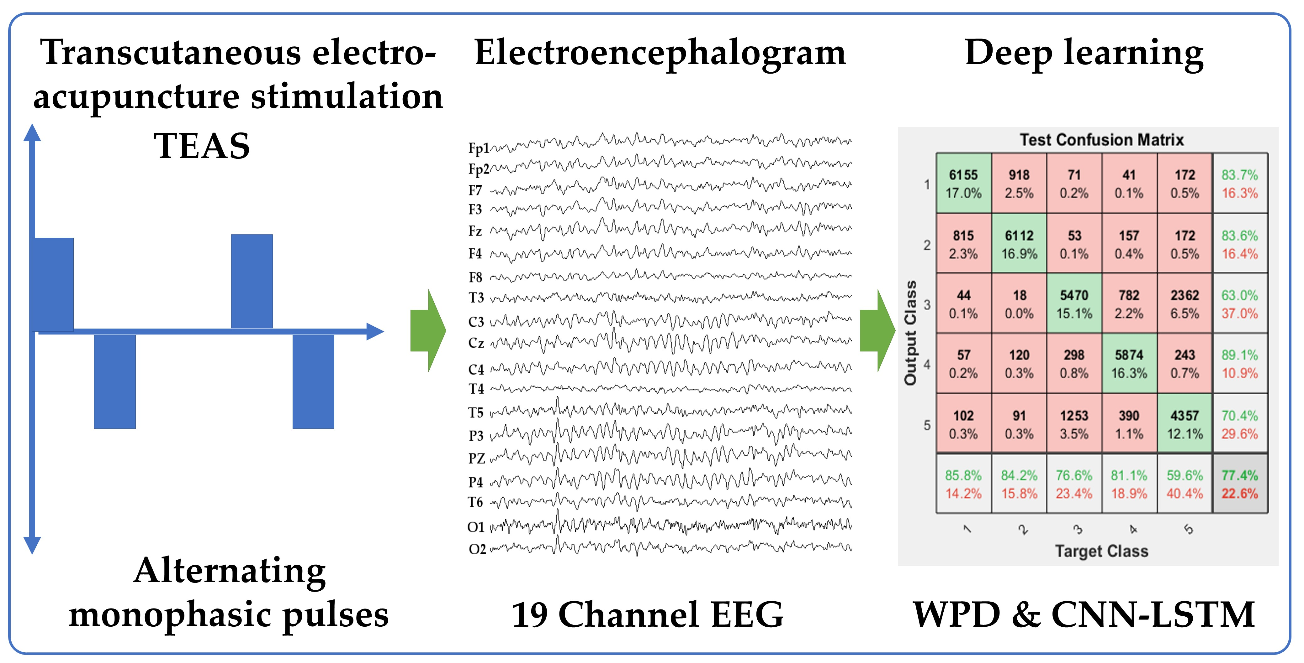
Based on a literature review, the authors of this study provide background information on artificial intelligence as used in EEG analysis, with an introduction to machine learning and deep learning methods for those—especially clinicians such as acupuncturists and physiotherapists—who may be unfamiliar with them. Summaries of the advantages and disadvantages of both ML and DL approaches are included, and also of some of their more commonly used algorithms. In addition, a literature review of EEG studies on acupuncture and related modalities was conducted. Based on these reviews, which, in themselves, provide a useful contribution to the literature, the authors used a combination of CNN (Convolutional Neural Network) and LSTM (Long Short-Term Memory) algorithms, as well as WPD (wavelet packet decomposition) for feature extraction.

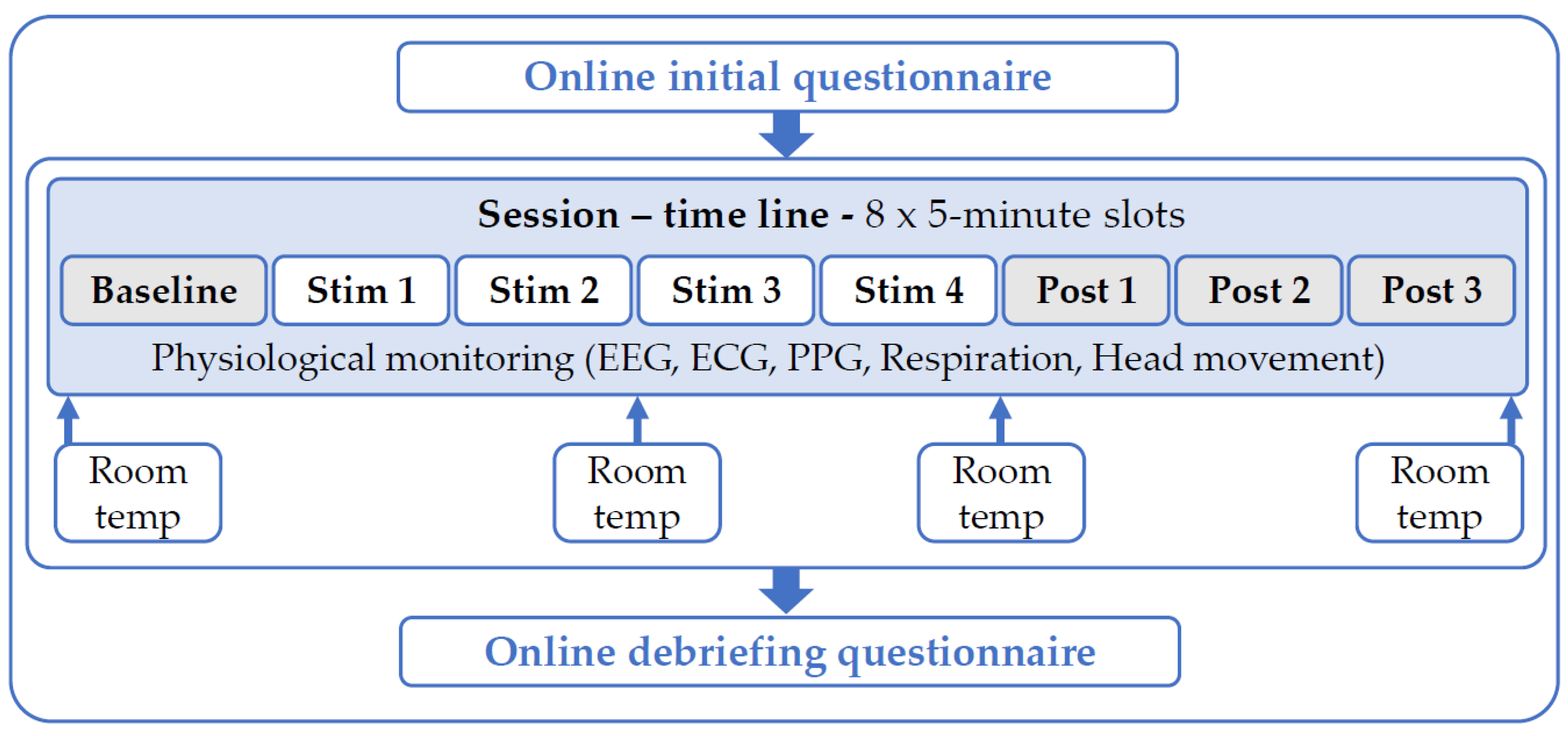
The experimental set-up was described, including TEAS, EEG data collection and pre-processing. We analysed the EEG data collected in four different ways (Phases 1 to 4):

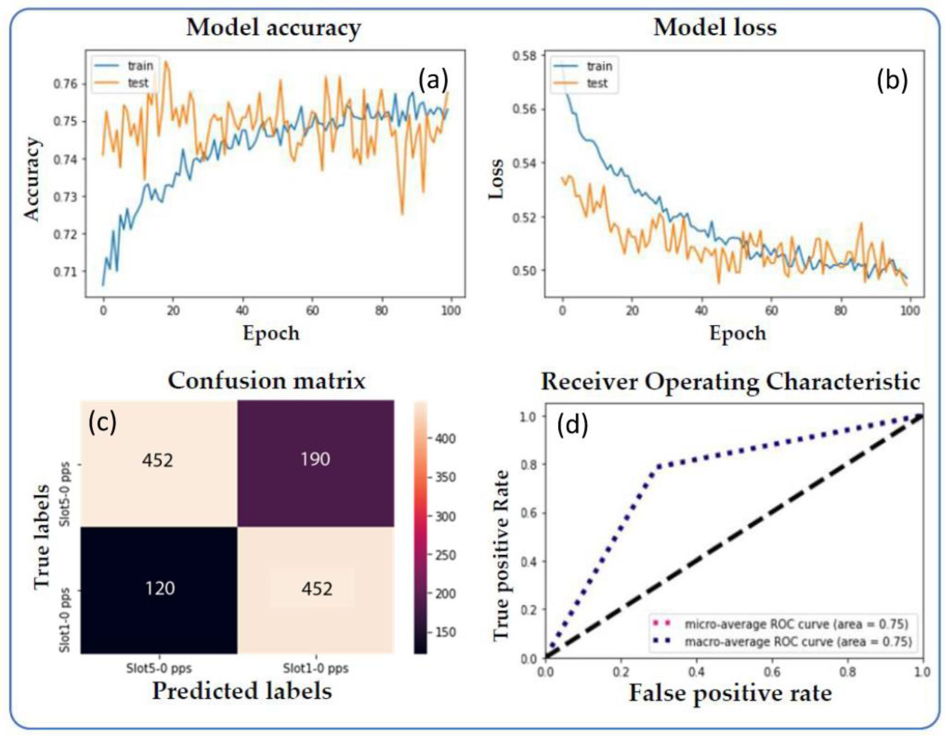
Phase 1. Sixteen hybrid CNN-LSTM models were created in Keras, to examine changes over time during stimulation (Slots 2, 3, 4 and 5) relative to the baseline (Slot 1), for each of the four stimulation frequencies, but without examining the filtered EEG bands separately. This resulted in 2 × 2 confusion matrices.

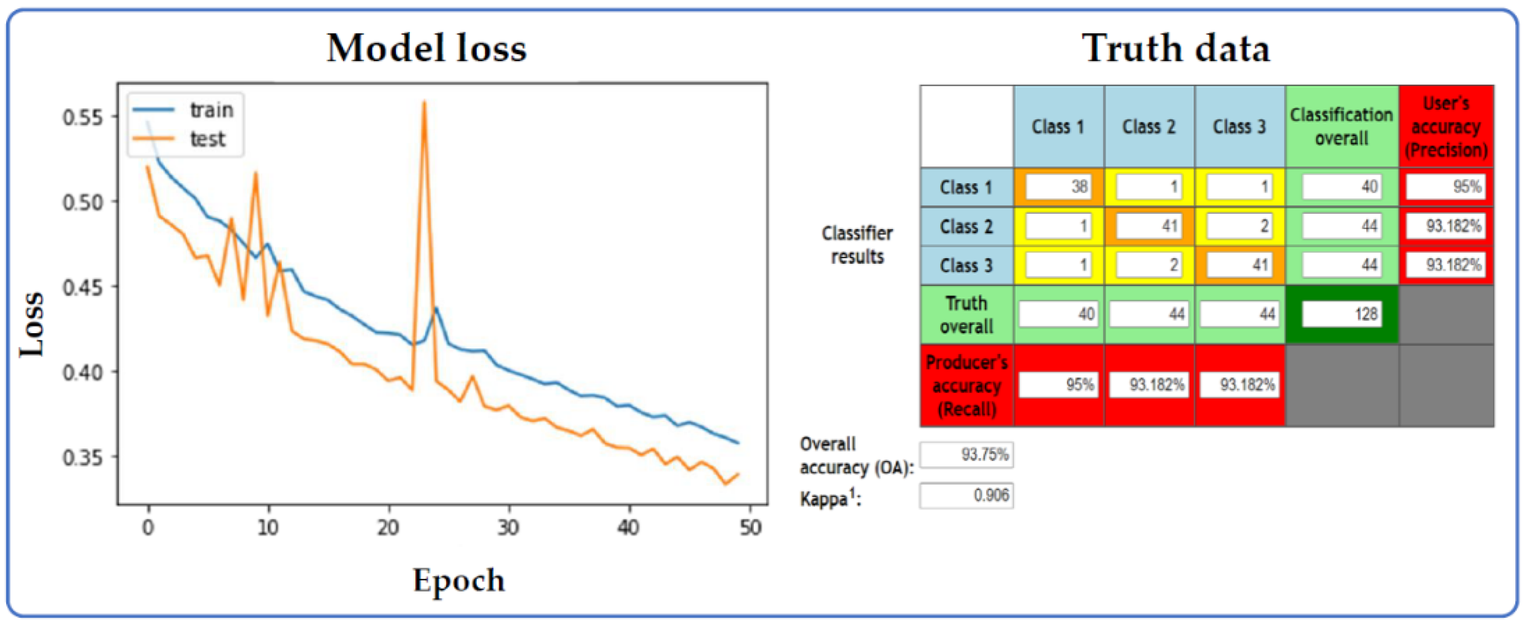
Phase 2. Twenty hybrid CNN-LSTM models were created in Keras, to examine changes over time (baseline (Slot 1), stimulation (Slots 2–5) and post-stimulation (Slots 6–8)) in each of the five EEG frequency bands (delta, theta, alpha, beta and gamma) for the four stimulation frequencies. This resulted in 3 × 3 confusion matrices.

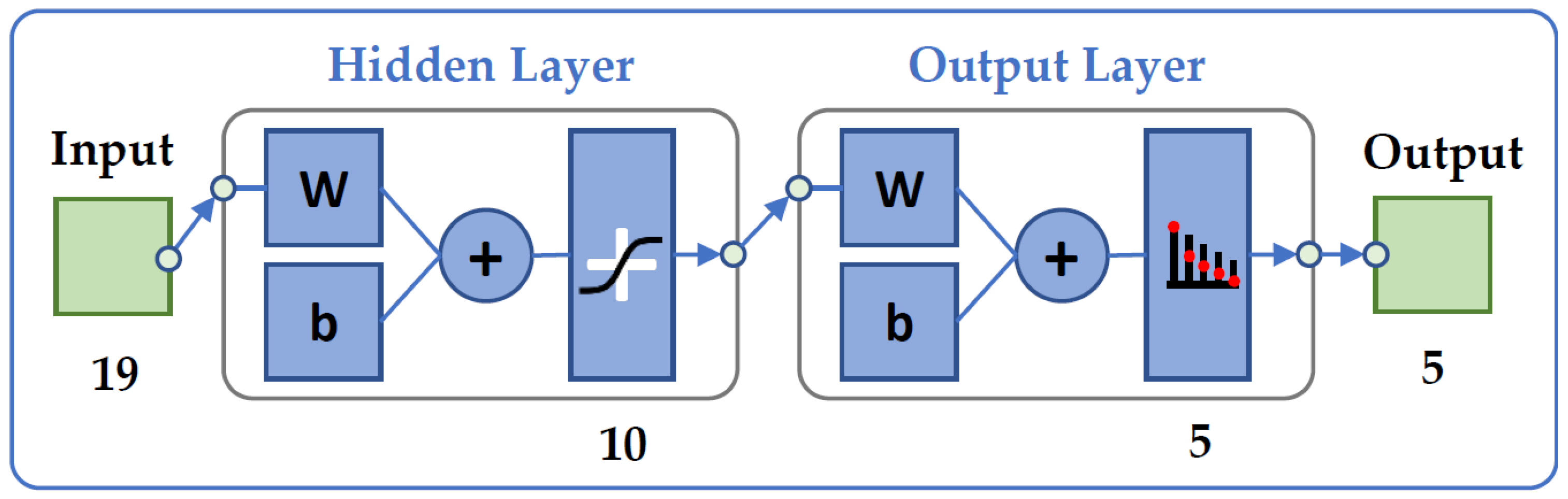
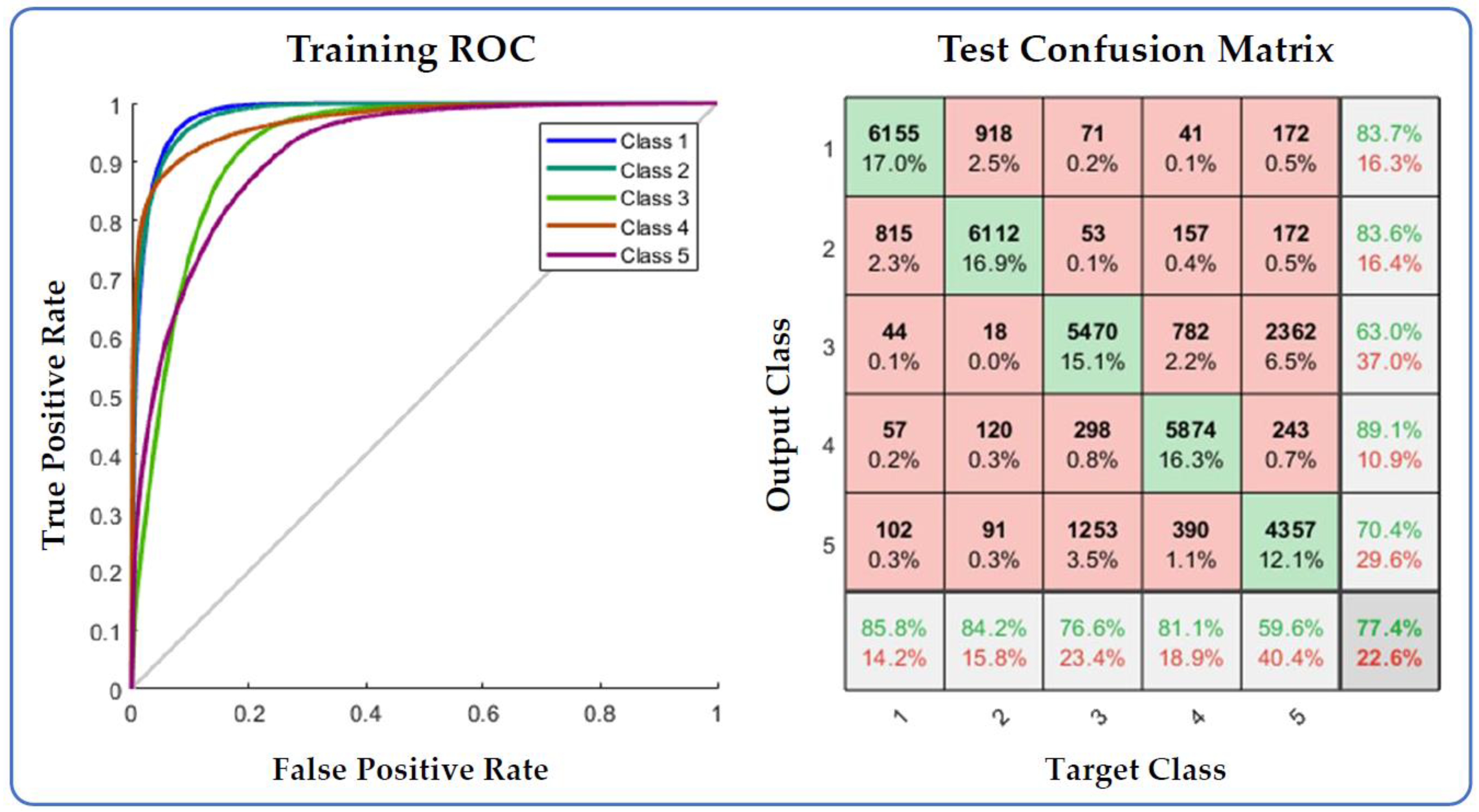
Phase 3. Twelve scaled conjugate backpropagation MLP-NN models with 10 hidden layers were created using MATLAB, to examine differences between the EEG bands at baseline, and during and following stimulation, for the four stimulation frequencies. This resulted in 5 × 5 confusion matrices.

Phase 4. Here, we reverted to using the CNN-LSTM model in Keras, rather as in Phase 1, but with more LSTM layers. The objective was to examine the same differences as in Phase 3, so that the two very different methods could be compared. Again, this resulted in 5*5 confusion matrices.

As with all (unsupervised) DL methods, however useful they may be in identifying and classifying differences, the results are not easy to interpret due to the complexity of the algorithms and the lack of a clear understanding of underlying mechanisms. This can be a major challenge in any study. Another potential challenge is that models may be prone to bias if the training data reflect biased patterns. A third challenge is in determining how to achieve computational efficiency.

The Phase 1 analysis appears to show that the greatest differences from the baseline occurred during 80 pps or sham stimulation, and the smallest differences during 2.5 or 10 pps stimulation. These results are plausible, if diametrically opposed to those that might be expected from the literature [17,18,19].

The phase 2 analysis suggests that differences between baseline, stimulation and post-stimulation EEG are greatest for 80 pps TEAS in the alpha band, and for 2.5 pps TEAS in the gamma band, with the smallest effect for 10 pps in alpha. The values of kappa showed greatest variance in Phase 2 analysis. Without knowing whether (and at which electrodes) these differences indicate increases or decreases in band power, or some other associated feature, these findings are hard to interpret. Would 2.5 pps TEAS be experienced as more stressful than 80 pps, for example, so that gamma power might increase with 2.5 pps stimulation, but alpha power with 80 pps? Further research is required to disentangle questions such as this.

The results of the Phase 3 analysis do not indicate major differences between any of the models, with the greatest differences among EEG bands at baseline for the sham and 2.5 pps TEAS, as well as for 2.5 pps post-stimulation. The Phase 4 results are quite different, with greatest differences among EEG bands, again, at baseline for 2.5 Hz TEAS, during stimulation for 10 pps and post-stimulation for 80 pps. However, differences among bands are to be expected, are not necessarily the result of stimulation and could be explained in many ways. None of the results from Phases 3 or 4 shed any light on the effects of stimulation frequency. It is of interest, though, that the mean and CV for kappa were considerably higher for the CNN-LSTM than for the MLP-NN model.

This assemblage of results provides a further useful contribution to the literature. However, in a world of limited resources that are increasingly under stress on many levels, an important general question is whether greater accuracy and precision should be prioritised over the energy-information costs incurred (solving a problem with a shallow structured network is always more advantageous in terms of computational burden if it can be solved). In what circumstances is a slightly fuzzy classification ‘good enough’? Here, the two models give different results, so perhaps, regardless of cost, those from the more computationally demanding model (CNN-LSTM) should be adopted, although which represents ‘ground truth’ is still a moot point. This may not always be the appropriate decision, and some may consider that the outcomes of this study do not justify the amount of energy and time it has taken to complete (almost 24 h in computation time for the AI algorithms alone, with another 12 h, approximately, for additional computation conducted using Google Colab in the cloud network). In conclusion, the software and hardware platforms used in deep learning operation are critical. Here, they were carefully selected to ensure accurate and reliable results. The inevitable human ‘wear-and-tear’ toll taken by intensive, collaborative research work should also be considered.

Some Limitations

The data were recorded in imperfect circumstances, in a laboratory that was not sound-proofed or temperature-controlled. Nonetheless, external noise was minimised as far as possible, and an attempt was made to keep the space at a comfortable temperature over the course of the year during which data were collected.

Our ‘sham’ (160 pps) TEAS was not completely without physiological effect, which may have biased our results. In retrospect, although various sham stimulation methods have been explored over the years by different researchers, some subthreshold and some suprathreshold [54,55,56], we should have amended our own experimental set-up to ensure no current whatsoever reached the participants. Unfortunately, we made a false assumption based on initial pilot experiments in which sham stimulation was, indeed, subthreshold for the test participants. This was not so for all those who took part in our final study. Nonetheless, the output was set to ‘zero’ on the Equinox device, so considerably lower during this imperfect sham stimulation than during the ‘active’ stimulations.

Only 66 participants took part in this study—a small dataset for a DL study. However, the use of training, validation and test sets, and of 5-fold validation, should have compensated for this.

In this paper, we did not tackle the question of whether our findings were the result of neural or volume conduction, or whether they indicated a central frequency-following response to peripheral stimulation. Moreover, our analysis did not investigate the EEG electrode-specific effects of TEAS, nor, indeed, the effects over different scalp regions. In addition, we did not explore how EEG might change during and following TEAS at different frequencies.

Unsupervised DL methods suffer from the problem of interpretability. This was exacerbated in the present study by communication difficulties between the clinicians and computer scientists involved, whom all had very different skills, mindsets, interests and languages. This project provided us all with a challenging and immersive learning experience. We hope not too many misinterpretations remain.

5. Conclusions

The application of DL to acupuncture-related research is a step change in the field and has the potential to greatly advance our understanding of the mechanisms and effects of acupuncture, as well as its clinical applications. By leveraging the power of DL algorithms, researchers can analyse and model large, complex datasets, identify patterns and relationships in the data that are not easily apparent through traditional statistical methods, and make predictions about the effects of acupuncture on various physiological responses.

This study is the first of its kind to use artificial intelligence to explore the effects of TEAS frequencies on EEG. From the published literature, no AI research appears to have been conducted into the effects on EEG of different frequencies of electroacupuncture-type stimulation (whether EA or TEAS), although there are several studies on the effects of manual needle rotation frequency from Tianjin University. Additionally, from the published literature, both WPD and the hybrid CNN-LSTM model appear to be appropriate methods of examining the central (EEG) effects of peripheral stimulation (TEAS). Using these methods, we found—contrary to expectation—that the greatest differences in EEG from baseline occurred during 80 pps or the ‘sham’ (160 pps) TEAS applied to the hands), with a mean kappa of 0.454 and 0.467, respectively, while the smallest differences occurred during 2.5 or 10 pps stimulation (mean kappa: 0.393 and 0.360). On the other hand, when taking the EEG bands into account, the greatest differences among Slot 1 (baseline)/Slots 2–5 (stimulation)/Slots 6–8 (post-stimulation) occurred for 2.5 pps TEAS in the Theta, Alpha and Gamma bands, and for 80 pps TEAS in Alpha (mean kappa 0.506). Even higher values of kappa were obtained from differences among the EEG bands before, during and after TEAS at different frequencies, but this result was difficult to interpret and explain, and warrants further exploration in future studies.

Future Directions

There are many potential avenues for further research based on the findings of this paper. Possible approaches could include conducting additional experiments to confirm or refute the findings of this study, as well as using different algorithms, different frequencies of TEAS, or different subject populations. Further research is planned using conventional methods of EEG analysis, different frequency bands (e.g., narrow bands centred on the stimulation frequencies), as well as ML methods based on careful feature selection, in order to see if the results obtained here can be replicated or improved—or, indeed, explained. Such features will include several connectivity (or graph theoretical) measures, including those of a source localisation method such as sLORETA (standardised low-resolution brain electromagnetic tomography), to investigate whether findings are due to neural or volume conduction, or, indeed, both. Changes over time both during and after stimulation should also be investigated for different TEAS frequencies. Changes due to volume conduction effects would only occur during, not after stimulation.

Because of the potentially large number of features that could be examined, automated feature selection is an option for use in this further investigation. EEG cordance and some topological measures have been computed for the current dataset. Although these results remain unpublished as yet, they may also be useful in guiding feature studies.

Furthermore, particular attention could be paid to entropy measures, whether in the time, frequency or spatial domain, as well as wavelet-based entropy using different entropy estimators, such as discrete wavelet entropy or permutation entropy. These entropy measures could potentially provide useful insights into the effects of different frequencies of TEAS on the brain, by quantifying the changes in the degree of disorder or uncertainty in the EEG signal.

Furthermore, future research protocols (1) could use EEG with a greater numbers of electrodes, (2) should ensure that ‘sham’ treatment is genuinely sham, and (3) could make use of further methods of data augmentation to strengthen effects. There is therefore scope for new research, such as that published here, that explores the effects of the frequency of TEAS on EEG using AI methods, with the most obvious place to start being a hybrid CNN-LSTM model. WPD also appears potentially suitable as a feature extraction method that could be used in conjunction with this type of DL model, if required (although, of course, one of the advantages of CNN is that feature extraction is performed by the algorithm itself, without prior handcrafting of features).

References

1. Walter, W.G.; Cooper, R.; Aldridge, V.J.; McCallum, W.C.; Winter, A.L. Contingent Negative Variation: An Electric Sign of Sensori-Motor Association and Expectancy in the Human Brain. Nature 1964, 203, 380–384. [Google Scholar] [CrossRef] [PubMed]
2. Mayor, D.; Bovey, M. An international survey on the current use of electroacupuncture. Acupunct. Med. 2017, 35, 30–37. [Google Scholar] [CrossRef] [PubMed]
3. Tang, Y.; Wang, L.; He, J.; Xu, Y.; Huang, S.; Fang, Y. Optimal Method of Electrical Stimulation for the Treatment of Upper Limb Dysfunction after Stroke: A Systematic Review and Bayesian Network Meta-Analysis of Randomized Controlled Trials. Neuropsychiatr. Dis. Treat. 2021, 17, 2937–2954. [Google Scholar] [CrossRef] [PubMed]
4. Chen, J.; Tu, Q.; Miao, S.; Zhou, Z.; Hu, S. Transcutaneous Electrical Acupoint Stimulation for Preventing Postoperative Nausea and Vomiting after General Anesthesia: A Meta-Analysis of Randomized Controlled Trials. Int. J. Surg. 2020, 73, 57–64. [Google Scholar] [CrossRef]
5. Chen, Z.; Wang, Y.; Wang, R.; Xie, J.; Ren, Y. Efficacy of Acupuncture for Treating Opioid Use Disorder in Adults: A Systematic Review and Meta-Analysis. Evid.-Based Complement. Altern. Med. 2018, 2018, 3724708. [Google Scholar] [CrossRef] [Green Version]
6. Ulett, G.A.; Han, S.; Han, J.S. Electroacupuncture: Mechanisms and Clinical Application. Biol. Psychiatry 1998, 44, 129–138. [Google Scholar] [CrossRef]
7. Napadow, V.; Makris, N.; Liu, J.; Kettner, N.W.; Kwong, K.K.; Hui, K.K.S. Effects of Electroacupuncture versus Manual Acupuncture on the Human Brain as Measured by fMRI. Hum. Brain Mapp. 2005, 24, 193–205. [Google Scholar] [CrossRef]
8. Wang, S.M.; Kain, Z.N.; White, P. Acupuncture Analgesia: I. The Scientific Basis. Anesth. Analg. 2008, 106, 602–610. [Google Scholar] [CrossRef]
9. Cummings, M. Safety Aspects of Electroacupuncture. Acupunct. Med. 2011, 29, 83–85. [Google Scholar] [CrossRef]
10. Tu, J.F.; Wang, L.Q.; Liu, J.H.; Qi, Y.S.; Tian, Z.X.; Wang, Y.; Yang, J.W.; Shi, G.X.; Kang, S.B.; Liu, C.Z. Home-based Transcutaneous Electrical Acupoint Stimulation for Hypertension: A Randomized Controlled Pilot Trial. Hypertens. Res. 2021, 44, 1300–1306. [Google Scholar] [CrossRef]
11. Yu, H.; Li, X.; Lei, X.; Wang, J. Modulation Effect of Acupuncture on Functional Brain Networks and Classification of Its Manipulation with EEG Signals. IEEE Trans. Neural Syst. Rehabil. Eng. 2019, 27, 1973–1984. [Google Scholar] [CrossRef] [PubMed]
12. Carraro, U. Thirty Years of Translational Research in Mobility Medicine: Collection of Abstracts of the 2020 Padua Muscle Days. Eur. J. Transl. Myol. 2020, 30, 3–47. [Google Scholar] [CrossRef] [PubMed]
13. Yin, T.; Ma, P.; Tian, Z.; Xie, K.; He, Z.; Sun, R.; Zeng, F. Machine Learning in Neuroimaging: A New Approach to Understand Acupuncture for Neuroplasticity. Neural Plast. 2020, 2020, 8871712. [Google Scholar] [CrossRef]
14. Kong, J.-T. Electroacupuncture for Treating Chronic Low-Back Pain: Preliminary Research Results. Med. Acupunct. 2020, 32, 396–397. [Google Scholar] [CrossRef] [PubMed]
15. Falagas, M.E.; Pitsouni, E.I.; Malietzis, G.A.; Pappas, G. Comparison of PubMed, Scopus, Web of Science, and Google Scholar: Strengths and Weaknesses. FASEB J. 2008, 22, 338–342. [Google Scholar] [CrossRef]
16. Boonyakitanont, P.; Lek-Uthai, A.; Songsiri, J. ScoreNet: A Neural Network-Based Post-Processing Model for Identifying Epileptic Seizure Onset and Offset in EEGs. IEEE Trans. Neural Syst. Rehabil. Eng. 2021, 29, 2474–2483. [Google Scholar] [CrossRef]
17. Han, J.S. Acupuncture: Neuropeptide Release Produced by Electrical Stimulation of Different Frequencies. Trends Neurosci. 2003, 26, 17–22. [Google Scholar] [CrossRef]
18. Mayor, D.F. How Electroacupuncture Works. I. Observations from Experimental and Animal Studies. In Electroacupuncture. A Practical Manual and Resource; Elsevier: Amsterdam, The Netherlands, 2007; pp. 59–76. [Google Scholar]
19. Mayor, D. An Exploratory Review of the Electroacupuncture Literature: Clinical Applications and Endorphin Mechanisms. Acupunct. Med. 2013, 31, 409–415. [Google Scholar] [CrossRef]
20. Dhond, R.P.; Kettner, N.; Napadow, V. Neuroimaging Acupuncture Effects in the Human Brain. J. Altern. Complement. Med. 2007, 13, 603–616. [Google Scholar] [CrossRef] [PubMed]
21. Rastiti, I.A.; Zheng, H.L.; Chen, C.L. Electroencephalogram Brain Connectome: An Approach in Research to Identify the Effect of Acupuncture on Human Brain Wave. World J. Tradit. Chin. Med. 2018, 4, 127–133. [Google Scholar] [CrossRef]
22. Gonzalez-Astudillo, J.; Cattai, T.; Bassignana, G.; Corsi, M.C.; De Vico Fallani, F. Network-Based Brain-Computer Interfaces: Principles and Applications. J. Neural Eng. 2021, 18. [Google Scholar] [CrossRef]
23. Li, N.; Wang, J.; Deng, B.; Dong, F. An Analysis of EEG When Acupuncture with Wavelet Entropy. In Proceedings of the 30th Annual International Conference of the IEEE Engineering in Medicine and Biology Society, EMBS’08—“Personalized Healthcare through Technology”, Vancouver, BC, Canada, 20–25 August 2008; pp. 1108–1111. [Google Scholar] [CrossRef]
24. Yi, G.; Wang, J.; Bian, H.; Han, C.; Deng, B.; Wei, X.; Li, H. Multi-Scale Order Recurrence Quantification Analysis of EEG Signals Evoked by Manual Acupuncture in Healthy Subjects. Cogn. Neurodynam. 2013, 7, 79–88. [Google Scholar] [CrossRef] [Green Version]
25. Pei, X.; Wang, J.; Deng, B.; Wei, X.; Yu, H. WLPVG Approach to the Analysis of EEG-Based Functional Brain Network under Manual Acupuncture. Cogn. Neurodynam. 2014, 8, 417–428. [Google Scholar] [CrossRef] [Green Version]
26. Wang, F.; Wang, H. Study of Driving Fatigue Alleviation by Transcutaneous Acupoints Electrical Stimulations. Sci. World J. 2014, 2014, 450249. [Google Scholar] [CrossRef] [PubMed] [Green Version]
27. Liu, Y.; Wu, X.; Feng, M. Extraction and Analysis of EEG Features under Electric Stimulation. In Proceedings of the ICMIPE 2013—2013 IEEE International Conference on Medical Imaging Physics and Engineering, Shenyang, China, 19–20 October 2013; IEEE Computer Society: Washington, DC, USA, 2013; pp. 254–258. [Google Scholar] [CrossRef]
28. Lee, T.W.; Girolami, M.; Sejnowski, T.J. Independent Component Analysis Using an Extended Infomax Algorithm for Mixed Subgaussian and Supergaussian Sources. Neural Comput. 1999, 11, 417–441. [Google Scholar] [CrossRef] [PubMed]
29. Winkler, I.; Haufe, S.; Tangermann, M. Automatic Classification of Artifactual ICA-Components for Artifact Removal in EEG Signals. Behav. Brain Funct. 2011, 7, 30. [Google Scholar] [CrossRef] [PubMed] [Green Version]
30. Pion-Tonachini, L.; Kreutz-Delgado, K.; Makeig, S. ICLabel: An Automated Electroencephalographic Independent Component Classifier, Dataset, and Website. Neuroimage 2019, 198, 181–197. [Google Scholar] [CrossRef] [Green Version]
31. Delorme, A.; Makeig, S. EEGLAB: An Open Source Toolbox for Analysis of Single-Trial EEG Dynamics Including Independent Component Analysis. J. Neurosci. Methods 2004, 134, 9–21. [Google Scholar] [CrossRef] [Green Version]
32. Lee, C.; Miyakoshi, M. TrimOutlier. 2022. Available online: https://github.com/sccn/trimOutlier (accessed on 17 December 2022).
33. Kayser, J.; Tenke, C.E. Principal Components Analysis of Laplacian Waveforms as a Generic Method for Identifying ERP Generator Patterns: I. Evaluation with Auditory Oddball Tasks. Clin. Neurophysiol. 2006, 117, 348–368. [Google Scholar] [CrossRef]
34. Chen, J.; Dou, Y.; Li, Y.; Li, J. Application of Shannon Wavelet Entropy and Shannon Wavelet Packet Entropy in Analysis of Power System Transient Signals. Entropy 2016, 18, 437. [Google Scholar] [CrossRef] [Green Version]
35. Saeidi, M.; Karwowski, W.; Farahani, F.V.; Fiok, K.; Taiar, R.; Hancock, P.A.; Al-Juaid, A. Neural Decoding of Eeg Signals with Machine Learning: A Systematic Review. Brain Sci. 2021, 11, 1525. [Google Scholar] [CrossRef] [PubMed]
36. Polikar, R. The Wavelet Tutorial Part III: Multiresolution Analysis & the Continuous Wavelet Transform; Iowa State University: Ames, IA, USA, 2004; pp. 1–28. Available online: http://cs.ucf.edu/courses/cap5015/WTpart3.pdf (accessed on 17 December 2022).
37. Khushaba, R.N.; Al-Jumaily, A.; Al-Ani, A. Novel Feature Extraction Method Based on Fuzzy Entropy and Wavelet Packet Transform for Myoelectric Control. In Proceedings of the ISCIT 2007—2007 International Symposium on Communications and Information Technologies Proceedings, Sydney, Australia, 17–19 October 2007; pp. 352–357. [Google Scholar] [CrossRef]
38. Khushaba, R.N.; Kodagoda, S.; Lal, S.; Dissanayake, G. Driver Drowsiness Classification Using Fuzzy Wavelet-Packet-Based Feature-Extraction Algorithm. IEEE Trans. Biomed. Eng. 2011, 58, 121–131. [Google Scholar] [CrossRef] [PubMed] [Green Version]
39. Khushaba, R. Feature Extraction Using Multisignal Wavelet Packet Decomposition. Available online: https://ch.mathworks.com/matlabcentral/fileexchange/33146-feature-extraction-using-multisignal-wavelet-packet-decomposition (accessed on 17 December 2022).
40. Amin, H.U.; Malik, A.S.; Ahmad, R.F.; Badruddin, N.; Kamel, N.; Hussain, M.; Chooi, W.T. Feature Extraction and Classification for EEG Signals Using Wavelet Transform and Machine Learning Techniques. Australas. Phys. Eng. Sci. Med. 2015, 38, 139–149. [Google Scholar] [CrossRef] [PubMed]
41. Uyulan, C.; Ergüzel, T.T.; Tarhan, N. Entropy-Based Feature Extraction Technique in Conjunction with Wavelet Packet Transform for Multi-Mental Task Classification. Biomed. Eng. Biomed. Tech. 2019, 64, 529–542. [Google Scholar] [CrossRef]
42. Rosso, O.A.; Blanco, S.; Yordanova, J.; Kolev, V.; Figliola, A.; Schürmann, M.; Başar, E. Wavelet Entropy: A New Tool for Analysis of Short Duration Brain Electrical Signals. J. Neurosci. Methods 2001, 105, 65–75. [Google Scholar] [CrossRef]
43. Uyulan, C.; Erguzel, T. Comparison of Wavelet Families for Mental Task Classification. J. Neurobehav. Sci. 2016, 3, 59. [Google Scholar] [CrossRef]
44. Daubechies, I. Orthonormal Bases of Compactly Supported Wavelets. Commun. Pure Appl. Math. 1988, 41, 909–996. [Google Scholar] [CrossRef] [Green Version]
45. Pedregosa, F.; Weiss, R.; Brucher, M.; Varoquaux, G.; Gramfort, A.; Michel, V.; Thirion, B.; Grisel, O.; Blondel, M.; Prettenhofer, P.; et al. Scikit-Learn: Machine Learning in Python. J. Mach. Learn. Res. 2011, 12, 2825–2830. [Google Scholar]
46. Géron, A. Hands-On Machine Learning with Scikit-Learn, Keras, and TensorFlow. Concepts, Tools, and Techniques to Build Intelligent Systems; O’Reilly Media: Sebastopol, CA, USA, 2017. [Google Scholar]
47. Fawcett, T. An Introduction to ROC Analysis. Pattern Recognit. Lett. 2006, 27, 861–874. [Google Scholar] [CrossRef]
48. Uyulan, C.; Erguzel, T.T. Analysis of Time—Frequency EEG Feature Extraction Methods for Mental Task Classification. Int. J. Comput. Intell. Syst. 2017, 10, 1280–1288. [Google Scholar] [CrossRef] [Green Version]
49. Erguzel, T.T.; Uyulan, C.; Unsalver, B.; Evrensel, A.; Cebi, M.; Noyan, C.O.; Metin, B.; Eryilmaz, G.; Sayar, G.H.; Tarhan, N. Entropy: A Promising EEG Biomarker Dichotomizing Subjects with Opioid Use Disorder and Healthy Controls. Clin. EEG Neurosci. 2020, 51, 373–381. [Google Scholar] [CrossRef] [PubMed]
50. MathWorks. Train and Apply Multilayer Shallow Neural Networks. Available online: https://uk.mathworks.com/help/deeplearning/ug/train-and-apply-multilayer-neural-networks.html (accessed on 3 March 2022).
51. Kiranyaz, S.; Avci, O.; Abdeljaber, O.; Ince, T.; Gabbouj, M.; Inman, D.J. 1D Convolutional Neural Networks and Applications: A Survey. Mech. Syst. Signal Process. 2021, 151, 107398. [Google Scholar] [CrossRef]
52. Landis, J.R.; Koch, G.G. An Application of Hierarchical Kappa-Type Statistics in the Assessment of Majority Agreement among Multiple Observers. Biometrics 1977, 33, 363–374. [Google Scholar] [CrossRef]
53. Landis, J.R.; Koch, G.G. The Measurement of Observer Agreement for Categorical Data. Biometrics 1977, 33, 159–174. [Google Scholar] [CrossRef] [PubMed] [Green Version]
54. Senin-Camargo, F.; Martínez-Rodríguez, A.; Chouza-Insua, M.; Raposo-Vidal, I.; Jácome, M.A. Effects on Venous Flow of Transcutaneous Electrical Stimulation, Neuromuscular Stimulation, and Sham Stimulation on Soleus Muscle: A Randomized Crossover Study in Healthy Subjects. Medicine 2022, 101, E30121. [Google Scholar] [CrossRef] [PubMed]
55. Namsawang, J.; Muanjai, P. Combined Use of Transcutaneous Electrical Nerve Stimulation and Short Foot Exercise Improves Navicular Height, Muscle Size, Function Mobility, and Risk of Falls in Healthy Older Adults. Int. J. Environ. Res. Public Health 2022, 19, 7196. [Google Scholar] [CrossRef]
56. Zarei, A.A.; Jensen, W.; Faghani Jadidi, A.; Lontis, E.R.; Atashzar, S.F. Gamma-Band Enhancement of Functional Brain Connectivity Following Transcutaneous Electrical Nerve Stimulation. J. Neural Eng. 2022, 19, 026020. [Google Scholar] [CrossRef]
57. Kaur, T.; Diwakar, A.; Kirandeep; Mirpuri, P.; Tripathi, M.; Chandra, P.; Gandhi, T. Artificial Intelligence in Epilepsy. Neurol. India 2021, 69, 560–566. [Google Scholar] [CrossRef]
58. Bell, J. Machine Learning: Hands-On for Developers and Technical Professionals; John Wiley & Sons: Indianapolis, IN, USA, 2015. [Google Scholar]
59. Mohammadpoor, M.; Shoeibi, A.; Shojaee, H. A Hierarchical Classification Method for Breast Tumor Detection. Iran. J. Med. Phys. 2016, 13, 261–268. [Google Scholar]
60. Bou Assi, E.; Nguyen, D.K.; Rihana, S.; Sawan, M. Towards Accurate Prediction of Epileptic Seizures: A Review. Biomed. Signal Process. Control 2017, 34, 144–157. [Google Scholar] [CrossRef]
61. Abbasi, B.; Goldenholz, D.M. Machine Learning Applications in Epilepsy. Epilepsia 2019, 60, 2037–2047. [Google Scholar] [CrossRef]
62. Vanschoren, J. Meta-Learning. In Automated Machine Learning: Methods, Systems, Challenges; Hutter, F., Kotthoff, L., Vanschoren, J., Eds.; The Springer Series on Challenges in Machine Learning; Springer Nature: Cham, Switzerland, 2019; pp. 35–62. [Google Scholar] [CrossRef] [Green Version]
63. Thornton, C.; Hutter, F.; Hoos, H.H.; Leyton-Brown, K. Auto-WEKA: Combined Selection and Hyperparameter Optimization of Classification Algorithms. In Proceedings of the ACM SIGKDD International Conference on Knowledge Discovery and Data Mining, Chicago, IL, USA, 11–14 August 2013; Association for Computing Machinery: New York, NY, USA, 2013; Volume F1288, pp. 847–855. [Google Scholar] [CrossRef]
64. Cortes, C.; Vapnik, V. Support-Vector Networks. Mach. Learn. 1995, 20, 273–297. [Google Scholar] [CrossRef]
65. Breiman, L.; Cutler, A. Random Forests. Available online: https://www.stat.berkeley.edu/~breiman/RandomForests/cc_home.htm#papers (accessed on 20 December 2021).
66. Fisher, R.A. The Use of Multiple Measurements in Taxonomic Problems. Ann. Eugen. 1936, 7, 179–188. [Google Scholar] [CrossRef]
67. Christodoulou, E.; Ma, J.; Collins, G.S.; Steyerberg, E.W.; Verbakel, J.Y.; Van Calster, B. A Systematic Review Shows No Performance Benefit of Machine Learning over Logistic Regression for Clinical Prediction Models. J. Clin. Epidemiol. 2019, 110, 12–22. [Google Scholar] [CrossRef] [PubMed]
68. Maimaiti, B.; Meng, H.; Lv, Y.; Qiu, J.; Zhu, Z.; Xie, Y.; Li, Y.; Cheng, Y.; Zhao, W.; Liu, J.; et al. An Overview of EEG-Based Machine Learning Methods in Seizure Prediction and Opportunities for Neurologists in This Field. Neuroscience 2022, 481, 197–218. [Google Scholar] [CrossRef] [PubMed]
69. Chauhan, V.K.; Dahiya, K.; Sharma, A. Problem Formulations and Solvers in Linear SVM: A Review. Artif. Intell. Rev. 2019, 52, 803–855. [Google Scholar] [CrossRef]
70. Sayah, F. Decision Trees and Random Forest for Beginners. Available online: https://www.kaggle.com/code/faressayah/decision-trees-random-forest-for-beginners/notebook (accessed on 17 December 2022).
71. Büyüköztürk, Ş.; Çokluk-Bökeoǧlu, Ö. Discriminant Function Analysis: Concept and Application. Egit. Arast. Eurasian J. Educ. Res. 2008, 33, 73–92. [Google Scholar]
72. Komarek, P.; Calvet, A. Logistic Regression for Data Mining and High-Dimensional Classificatiom. J. Allergy Clin. Immunol. 2004, 130, 556. [Google Scholar]
73. Bießmann, F.; Plis, S.; Meinecke, F.C.; Eichele, T.; Müller, K.R. Analysis of Multimodal Neuroimaging Data. IEEE Rev. Biomed. Eng. 2011, 4, 26–58. [Google Scholar] [CrossRef]
74. Barros, C.; Silva, C.A.; Pinheiro, A.P. Advanced EEG-Based Learning Approaches to Predict Schizophrenia: Promises and Pitfalls. Artif. Intell. Med. 2021, 114, 102039. [Google Scholar] [CrossRef]
75. Brownlee, J. A Tour of Machine Learning Algorithms. Available online: https://machinelearningmastery.com/a-tour-of-machine-learning-algorithms/ (accessed on 17 December 2022).
76. Kumar, V. A Hands-on Guide To Hybrid Ensemble Learning Models, with Python Code. Dev. CORNER 2020. Available online: https://analyticsindiamag.com/a-hands-on-guide-to-hybrid-ensemble-learning-models-with-python-code/ (accessed on 17 December 2022).
77. Hawkins, D.M. The Problem of Overfitting. J. Chem. Inf. Comput. Sci. 2004, 44, 1–12. [Google Scholar] [CrossRef] [PubMed]
78. Yenugula, J. How to Handle Overfitting with Regularization. Available online: https://dataaspirant.com/handle-overfitting-with-regularization/#t-1610645875806 (accessed on 17 December 2022).
79. Brownlee, J. How to Choose an Activation Function for Deep Learning. Mach. Learn. Mastery 2021, 1–26. Available online: https://machinelearningmastery.com/choose-an-activation-function-for-deep-learning/ (accessed on 17 December 2022).
80. Lazzeri, F. How to Accelerate DevOps with Machine Learning Lifecycle Management. Available online: https://medium.com/microsoftazure/how-to-accelerate-devops-with-machine-learning-lifecycle-management-2ca4c86387a0 (accessed on 17 December 2022).
81. Wikipedia Contributors. Feature Selection. Available online: https://en.wikipedia.org/wiki/Feature_selection (accessed on 17 December 2022).
82. Brownlee, J. Introduction to Dimensionality Reduction for Machine Learning. Available online: https://machinelearningmastery.com/dimensionality-reduction-for-machine-learning/ (accessed on 17 December 2022).
83. Brownlee, J. What is the Difference between A Parameter and A Hyperparameter? Available online: https://machinelearningmastery.com/difference-between-a-parameter-and-a-hyperparameter/ (accessed on 28 February 2022).
84. Brownlee, J. Train-Test Split for Evaluating Machine Learning Algorithms. Available online: https://machinelearningmastery.com/train-test-split-for-evaluating-machine-learning-algorithms/ (accessed on 17 December 2022).
85. Brownlee, J. A Simple Intuition for Overfitting, or Why Testing on Training Data is a Bad Idea. Available online: https://machinelearningmastery.com/a-simple-intuition-for-overfitting/ (accessed on 1 March 2022).
86. Wikipedia Contributors. Training, Validation, and Test Data Sets. Available online: https://en.wikipedia.org/wiki/Training,_validation,_and_test_data_sets (accessed on 1 December 2022).
87. Ng, A. Train, Validate, and Test. Available online: http://primo.ai/index.php?title=Train,_Validate,_and_Test (accessed on 17 December 2022).
88. Tulay, E.E.; Metin, B.; Tarhan, N.; Arıkan, M.K. Multimodal Neuroimaging: Basic Concepts and Classification of Neuropsychiatric Diseases. Clin. EEG Neurosci. 2019, 50, 20–33. [Google Scholar] [CrossRef] [PubMed]
89. Chamola, V.; Vineet, A.; Nayyar, A.; Hossain, E. Brain-Computer Interface-Based Humanoid Control: A Review. Sensors 2020, 20, 3620. [Google Scholar] [CrossRef] [PubMed]
90. Gupta, S. Pros and Cons of Various Machine Learning Algorithms. Available online: https://towardsdatascience.com/pros-and-cons-of-various-classification-ml-algorithms-3b5bfb3c87d6 (accessed on 17 December 2022).
91. Ray, S. A Quick Review of Machine Learning Algorithms. In Proceedings of the International Conference on Machine Learning, Big Data, Cloud and Parallel Computing: Trends, Prespectives and Prospects, (COMITCon 2019), Faridabad, India, 14–16 February 2019; pp. 35–39. [Google Scholar] [CrossRef]
92. Tahernezhad-Javazm, F.; Azimirad, V.; Shoaran, M. A Review and Experimental Study on the Application of Classifiers and Evolutionary Algorithms in EEG-Based Brain-Machine Interface Systems. J. Neural Eng. 2018, 15, 021007. [Google Scholar] [CrossRef] [PubMed]
93. Baeldung. Multiclass Classification Using Support Vector Machines. Available online: https://www.baeldung.com/cs/svm-multiclass-classification (accessed on 20 December 2021).
94. Adebowale, A.; Idowu, S.A.; Amarachi, A.A. Comparative Study of Selected Data Mining Algorithms Used For Intrusion Detection. Int. J. Soft Comput. Eng. 2013, 3, 237–241. [Google Scholar]
95. Drucker, H.; Surges, C.J.C.; Kaufman, L.; Smola, A.; Vapnik, V. Support Vector Regression Machines. In Advances in Neural Information Processing Systems; MIT Press: Cambridge, MA, USA, 1997; pp. 155–161. [Google Scholar]
96. Kalcheva, N.; Todorova, M.; Marinova, G. Naive Bayes Classifier, Decision Tree and AdaBoost Ensemble Algorithm–Advantages and Disadvantages. In Proceedings of the 6th ERAZ Conference Proceedings (part of ERAZ conference collection), Online, 21 May 2020; pp. 153–157. [Google Scholar] [CrossRef]
97. Lotte, F.; Bougrain, L.; Cichocki, A.; Clerc, M.; Congedo, M.; Rakotomamonjy, A.; Yger, F. A Review of Classification Algorithms for EEG-Based Brain-Computer Interfaces: A 10 Year Update. J. Neural Eng. 2018, 15, 031005. [Google Scholar] [CrossRef] [PubMed] [Green Version]
98. Brownlee, J. TensorFlow 2 Tutorial: Get Started in Deep Learning with tf.keras. Available online: https://machinelearningmastery.com/tensorflow-tutorial-deep-learning-with-tf-keras/ (accessed on 17 December 2022).
99. Wikipedia Contributors. Talk: Linear Discriminant Analysis. Available online: https://en.wikipedia.org/wiki/Talk%3ALinear_discriminant_analysis (accessed on 17 December 2022).
100. Brownlee, J. Linear Discriminant Analysis for Machine Learning. Mach. Learn. Mastery 2016, 6. Available online: https://machinelearningmastery.com/linear-discriminant-analysis-for-machine-learning/ (accessed on 17 December 2022).
101. Brownlee, J. What is a Confusion Matrix in Machine Learning. Available online: https://machinelearningmastery.com/confusion-matrix-machine-learning/ (accessed on 17 December 2022).
102. Sharma, P.; Kaur, M. Classification in Pattern Recognition: A Review. Int. J. Adv. Res. Comput. Sci. Softw. Eng. 2013, 3, 298–306. [Google Scholar]
103. Bujang, M.A.; Sa’At, N.; Tg Abu Bakar Sidik, T.M.I.; Lim, C.J. Sample Size Guidelines for Logistic Regression from Observational Studies with Large Population: Emphasis on the Accuracy between Statistics and Parameters Based on Real Life Clinical Data. Malays. J. Med. Sci. 2018, 25, 122–130. [Google Scholar] [CrossRef]
104. Ding, C.; He, X. K-Nearest-Neighbor Consistency in Data Clustering: Incorporating Local Information into Global Optimization. In Proceedings of the ACM Symposium on Applied Computing, Nicosia, Cyprus, 14–17 March 2004; Volume 1, pp. 584–589. [Google Scholar]
105. Omran, M.G.H.; Engelbrecht, A.P.; Salman, A. An Overview of Clustering Methods. Intell. Data Anal. 2007, 11, 583–605. [Google Scholar] [CrossRef]
106. i2tutorials. What are the Pros and Cons of the PCA? Available online: https://www.i2tutorials.com/what-are-the-pros-and-cons-of-the-pca/ (accessed on 20 December 2021).
107. Devi, T.S.; Sundaram, K.M. A Comparative Analysis of Meta and Tree Classification Algorithms using WEKA. Int. Res. J. Eng. Technol. 2016, 3, 77–83. [Google Scholar]
108. Stancin, I.; Cifrek, M.; Jovic, A. A Review of EEG Signal Features and Their Application in Driver Drowsiness Detection Systems. Sensors 2021, 21, 3786. [Google Scholar] [CrossRef] [PubMed]
109. Leuchter, A.F.; Cook, I.A.; Hamilton, S.P.; Narr, K.L.; Toga, A.; Hunter, A.M.; Faull, K.; Whitelegge, J.; Andrews, A.M.; Loo, J.; et al. Biomarkers to Predict Antidepressant Response. Curr. Psychiatry Rep. 2010, 12, 553–562. [Google Scholar] [CrossRef] [Green Version]
110. Michel, C.M.; Koenig, T. EEG Microstates as a Tool for Studying the Temporal Dynamics of Whole-Brain Neuronal Networks: A Review. Neuroimage 2018, 180, 577–593. [Google Scholar] [CrossRef]
111. Kleifges, K.; Bigdely-Shamlo, N.; Kerick, S.E.; Robbins, K.A. BLINKER: Automated Extraction of Ocular Indices from EEG Enabling Large-Scale Analysis. Front. Neurosci. 2017, 11, 12. [Google Scholar] [CrossRef] [Green Version]
112. Rampil, I.J.; Sasse, F.J.; Smith, N.T. Spectral Edge Frequency: A New Correlate of Anesthetic Depth. Anesthesiology 1980, 53 (Suppl. 3), S12. [Google Scholar] [CrossRef]
113. Lehmann, D.; Strik, W.K.; Henggeler, B.; Koenig, T.; Koukkou, M. Brain Electric Microstates and Momentary Conscious Mind States as Building Blocks of Spontaneous Thinking: I. Visual Imagery and Abstract Thoughts. Int. J. Psychophysiol. 1998, 29, 1–11. [Google Scholar] [CrossRef]
114. Oliveira, C.R.D.; Bernardo, W.M.; Nunes, V.M. Benefit of General Anesthesia Monitored by Bispectral Index Compared with Monitoring Guided Only by Clinical Parameters. Systematic Review and Meta-analysis. Braz. J. Anesthesiol. 2017, 67, 72–84. [Google Scholar] [CrossRef] [Green Version]
115. Carbone, F.; Alberti, T.; Faranda, D.; Telloni, D.; Consolini, G.; Sorriso-Valvo, L. Local Dimensionality and Inverse Persistence Analysis of Atmospheric Turbulence in the Stable Boundary Layer. Phys. Rev. E 2022, 106, 064211. [Google Scholar] [CrossRef]
116. Santos, E.M.; San-Martin, R.; Fraga, F.J. Comparison of LORETA and CSP for Brain-Computer Interface Applications. In Proceedings of the 18th IEEE International Multi-Conference on Systems, Signals and Devices, SSD, Monastir, Tunisia, 22–25 March 2021; pp. 817–822. [Google Scholar] [CrossRef]
117. Linting, M. Nonparametric Inference in Nonlinear Principal Components Analysis: Exploration and Beyond; Leiden UniversityScholarly Publications: Leiden, The Netherlands, 2007. [Google Scholar]
118. Long, J.S.; Freese, J. Regression Models for Categorical Dependent Variables Using Stata, 3rd ed.; Stata Press: College Station, TX, USA, 2014. [Google Scholar]
119. Chicco, D.; Jurman, G. The Advantages of the Matthews Correlation Coefficient (MCC) over F1 Score and Accuracy in Binary Classification Evaluation. BMC Genom. 2020, 21, 6. [Google Scholar] [CrossRef] [PubMed] [Green Version]
120. Chicco, D.; Warrens, M.J.; Jurman, G. The Matthews Correlation Coefficient (MCC) Is More Informative Than Cohen’s Kappa and Brier Score in Binary Classification Assessment. IEEE Access 2021, 9, 78368–78381. [Google Scholar] [CrossRef]
121. Vanetti, M. Confusion Matrix Online Calculator. Available online: https://scholar.google.com/scholar?hl=en&as_sdt=0%2C5&q=Vanetti+M.+n.d.+Confusion+matrix+online+calculator.&btnG= (accessed on 17 December 2022).
122. Stack Exchange. Cohen’s Kappa in Plain English. Available online: https://stats.stackexchange.com/questions/82162/cohens-kappa-in-plain-english (accessed on 23 February 2022).
123. Khosla, A.; Khandnor, P.; Chand, T. EEG-Based Automatic Multi-Class Classification of Epileptic Seizure Types Using Recurrence Plots. Expert Syst. 2022, 39, e12923. [Google Scholar] [CrossRef]
124. Goodfellow, I.; Bengio, Y.; Courville, A. Book Review: Deep Learning. Healthc. Inform. Res. 2016, 22, 351–354. [Google Scholar] [CrossRef] [Green Version]
125. Van Rijn, J.N.; Hutter, F. Hyperparameter Importance across Datasets. In Proceedings of the ACM SIGKDD International Conference on Knowledge Discovery and Data Mining, London, UK, 19–23 August 2018; ACM: New York, NY, USA, 2018; pp. 2367–2376. [Google Scholar] [CrossRef] [Green Version]
126. Kotthoff, L.; Thornton, C.; Hoos, H.H.; Hutter, F.; Leyton-Brown, K. Auto-WEKA 2.0: Automatic Model Selection and Hyperparameter Optimization in WEKA. In Automated Machine Learning; Springer: Cham, Switzerland, 2017; pp. 81–95. [Google Scholar] [CrossRef] [Green Version]
127. Feurer, M.; Klein, A.; Eggensperger, K.; Springenberg, J.T.; Blum, M.; Hutter, F. Efficient and Robust Automated Machine Learning. In Advances in Neural Information Processing Systems; MIT Press: Cambridge, MA, USA, 2015; pp. 2962–2970. [Google Scholar]
128. Jin, H.; Song, Q.; Hu, X. Auto-Keras: An Efficient Neural Architecture Search System. In Proceedings of the ACM SIGKDD International Conference on Knowledge Discovery and Data Mining, New York, NY, USA, 4–8 August 2019; Association for Computing Machinery: New York, NY, USA, 2019; pp. 1946–1956. [Google Scholar] [CrossRef] [Green Version]
129. Acharya, U.R.; Oh, S.L.; Hagiwara, Y.; Tan, J.H.; Adeli, H.; Subha, D.P. Automated EEG-Based Screening of Depression Using Deep Convolutional Neural Network. Comput. Methods Programs Biomed. 2018, 161, 103–113. [Google Scholar] [CrossRef]
130. Alzahab, N.A.; Apollonio, L.; Di Iorio, A.; Alshalak, M.; Iarlori, S.; Ferracuti, F.; Monteriù, A.; Porcaro, C. Hybrid Deep Learning (HDL)-Based Brain-Computer Interface (BCI) Systems: A Systematic Review. Brain Sci. 2021, 11, 75. [Google Scholar] [CrossRef] [PubMed]
131. Bakar, A.R.A.; Lai, K.W.; Hamzaid, N.A. The Emergence of Machine Learning in Auditory Neural Impairment: A Systematic Review. Neurosci. Lett. 2021, 765, 136250. [Google Scholar] [CrossRef]
132. Craik, A.; He, Y.; Contreras-Vidal, J.L. Deep Learning for Electroencephalogram (EEG) Classification Tasks: A Review. J. Neural Eng. 2019, 16, 031001. [Google Scholar] [CrossRef] [PubMed]
133. Ko, W.; Jeon, E.; Jeong, S.; Phyo, J.; Suk, H.I. A Survey on Deep Learning-Based Short/Zero-Calibration Approaches for EEG-Based Brain–Computer Interfaces. Front. Hum. Neurosci. 2021, 15, 643386. [Google Scholar] [CrossRef]
134. Rasheed, K.; Qayyum, A.; Qadir, J.; Sivathamboo, S.; Kwan, P.; Kuhlmann, L.; O’Brien, T.; Razi, A. Machine Learning for Predicting Epileptic Seizures Using EEG Signals: A Review. IEEE Rev. Biomed. Eng. 2021, 14, 139–155. [Google Scholar] [CrossRef]
135. Heidari, A.; Jafari Navimipour, N.; Unal, M.; Toumaj, S. The COVID-19 Epidemic Analysis and Diagnosis Using Deep Learning: A Systematic Literature Review and Future Directions. Comput. Biol. Med. 2022, 141, 105141. [Google Scholar] [CrossRef]
136. Guilenea, F.N.; Casciaro, M.E.; Pascaner, A.F.; Soulat, G.; Mousseaux, E.; Craiem, D. Thoracic Aorta Calcium Detection and Quantification Using Convolutional Neural Networks in a Large Cohort of Intermediate-Risk Patients. Tomography 2021, 7, 636–649. [Google Scholar] [CrossRef]
137. Xiao, Y.; Chen, Y.; Wang, Z. Secure Transmission of W-Band Millimeter-Wave Based on CNN and Dynamic Resource Allocation. Opt. Lett. 2021, 46, 5583–5586. [Google Scholar] [CrossRef] [PubMed]
138. Movahedi, F.; Coyle, J.L.; Sejdic, E. Deep Belief Networks for Electroencephalography: A Review of Recent Contributions and Future Outlooks. IEEE J. Biomed. Health Inform. 2018, 22, 642–652. [Google Scholar] [CrossRef]
139. Mu, R.; Zeng, X. A Review of Deep Learning Research. KSII Trans. Internet Inf. Syst. 2019, 13, 1738–1764. [Google Scholar] [CrossRef]
140. Yu, Y.; Si, X.; Hu, C.; Zhang, J. A Review of Recurrent Neural Networks: LSTM Cells and Network Architectures. Neural Comput. 2019, 31, 1235–1270. [Google Scholar] [CrossRef]
141. Ganaie, M.A.; Hu, M.; Malik, A.K.; Tanveer, M.; Suganthan, P.N. Ensemble Deep Learning: A Review. Eng. Appl. Artif. Intell. 2022, 115, 105151. [Google Scholar] [CrossRef]
142. Goodfellow, I.; Pouget-Abadie, J.; Mirza, M.; Xu, B.; Warde-Farley, D.; Ozair, S.; Courville, A.; Bengio, Y. Generative Adversarial Networks. Commun. ACM 2020, 63, 139–144. [Google Scholar] [CrossRef]
143. Iwana, B.K.; Uchida, S. An Empirical Survey of Data Augmentation for Time Series Classification with Neural Networks. PLoS ONE 2021, 16, e0254841. [Google Scholar] [CrossRef] [PubMed]
144. Lashgari, E.; Liang, D.; Methods, U.M. Data Augmentation for Deep-Learning-Based Electroencephalography. J. Neurosci. Methods 2020, 346, 108885. [Google Scholar] [CrossRef]
145. Voulodimos, A.; Doulamis, N.; Doulamis, A.; Protopapadakis, E. Deep Learning for Computer Vision: A Brief Review. Comput. Intell. Neurosci. 2018, 2018, 7068349. [Google Scholar] [CrossRef]
146. Faust, O.; Hagiwara, Y.; Hong, T.J.; Lih, O.S.; Acharya, U.R. Deep Learning for Healthcare Applications Based on Physiological Signals: A Review. Comput. Methods Programs Biomed. 2018, 161, 1–13. [Google Scholar] [CrossRef]
147. da Silva Lourenço, C.; Tjepkema-Cloostermans, M.C.; van Putten, M.J.A.M. Machine Learning for Detection of Interictal Epileptiform Discharges. Clin. Neurophysiol. 2021, 132, 1433–1443. [Google Scholar] [CrossRef]
148. Schirrmeister, R.T.; Springenberg, J.T.; Fiederer, L.D.J.; Glasstetter, M.; Eggensperger, K.; Tangermann, M.; Hutter, F.; Burgard, W.; Ball, T. Deep Learning with Convolutional Neural Networks for EEG Decoding and Visualization. Hum. Brain Mapp. 2017, 38, 5391–5420. [Google Scholar] [CrossRef] [Green Version]
149. Ma, X.; Qiu, S.; Du, C.; Xing, J.; He, H. Improving EEG-Based Motor Imagery Classification via Spatial and Temporal Recurrent Neural Networks. In Proceedings of the Annual International Conference of the IEEE Engineering in Medicine and Biology Society, EMBS, Honolulu, HI, USA, 18–21 July 2018; Volume 2018, pp. 1903–1906. [Google Scholar] [CrossRef]
150. Freedman, R. LSTM and Extended Dead Reckoning Automobile Route Prediction Using Smartphone Sensors. Master’s Thesis, University of Illinois at Urbana-Champaign, Champaign, IL, USA, 2017. [Google Scholar]
151. Gopan, K.G.; Reddy, S.V.R.A.; Rao, M.; Sinha, N. Analysis of Single Channel Electroencephalographic Signals for Visual Creativity: A Pilot Study. Biomed. Signal Process. Control 2022, 75, 103542. [Google Scholar] [CrossRef]
152. Feng, T. Deep Learning for Depth, Ego-Motion, Optical Flow Estimation, and Semantic Segmentation. Ph.D. Thesis, School of Computer Science and Electronic Engineering, University of Essex, Colchester, UK, 2021. Available online: https://repository.essex.ac.uk/31706/1/University_of_Essex_PhD_THESIS_Tuo.pdf (accessed on 17 December 2022).
153. Pathak, P.; Poudel, P.; Roy, S.; Caragea, D. Leveraging Attention-Based Deep Neural Networks for Security Vetting of Android Applications. ICST Trans. Secur. Saf. 2021, 8, 171168. [Google Scholar] [CrossRef]
154. Cui, F.; Yue, Y.; Zhang, Y.; Zhang, Z.; Zhou, H.S. Advancing Biosensors with Machine Learning. ACS Sens. 2020, 5, 3346–3364. [Google Scholar] [CrossRef] [PubMed]
155. Vijaykumar, S.; Swathi, S.; Upperkar, R. Deep Learning: A New Paradigm to Machine Learning. Int. J. Sci. Res. Comput. Sci. Appl. Manag. Stud. 2020, 9. Available online: https://www.ijsrcsams.com/images/stories/Past_Issue_Docs/ijsrcsamsv9i1p12.pdf (accessed on 17 December 2022).
156. Qian, Y.; Fan, Y.; Hu, W.; Soong, F.K. On the Training Aspects of Deep Neural Network (DNN) for Parametric TTS Synthesis. In Proceedings of the ICASSP—IEEE International Conference on Acoustics, Speech and Signal Processing, Florence, Italy, 4–9 May 2014; pp. 3829–3833. [Google Scholar] [CrossRef]
157. Xiong, B.; Meng, X.; Wang, R.; Wang, X.; Wang, Z. Combined Model for Short-Term Wind Power Prediction Based on Deep Neural Network and Long Short-Term Memory. J. Phys. Conf. Ser. 2021, 1757, 012095. [Google Scholar] [CrossRef]
158. Montavon, G.; Samek, W.; Müller, K.R. Methods for Interpreting and Understanding Deep Neural Networks. Digit. Signal Process. A Rev. J. 2018, 73, 1–15. [Google Scholar] [CrossRef]
159. Klampanos, I.A.; Davvetas, A.; Andronopoulos, S.; Pappas, C.; Ikonomopoulos, A.; Karkaletsis, V. Autoencoder-Driven Weather Clustering for Source Estimation during Nuclear Events. Environ. Model. Softw. 2018, 102, 84–93. [Google Scholar] [CrossRef] [Green Version]
160. Yu, T.; Zhu, H. Hyper-Parameter Optimization: A Review of Algorithms and Applications. arXiv 2020, arXiv:2003.05689. [Google Scholar] [CrossRef]
161. Zaheer, R.; Shaziya, H. A Study of the Optimization Algorithms in Deep Learning. In Proceedings of the 3rd International Conference on Inventive Systems and Control, ICISC 2019, Coimbatore, India, 10–11 January 2019; Institute of Electrical and Electronics Engineers Inc.: Piscataway, NJ, USA, 2019; pp. 536–539. [Google Scholar] [CrossRef]
162. Haji, S.H.; Abdulazeez, A.M. Comparison of Optimization Techniques Based on Gradient Descent Algorithm: A Review. PalArch’s J. Archaeol. Egypt/Egyptol. 2021, 18, 2715–2743. [Google Scholar]
163. Li, G.; Lee, C.H.; Jung, J.J.; Youn, Y.C.; Camacho, D. Deep Learning for EEG Data Analytics: A Survey. In Concurrency and Computation: Practice and Experience; John Wiley and Sons Ltd.: Hoboken, NJ, USA, 2020; Volume 32. [Google Scholar] [CrossRef]
164. Brena, R.F.; Aguileta, A.A.; Trejo, L.A.; Molino-Minero-Re, E.; Mayora, O. Choosing the Best Sensor Fusion Method: A Machine-Learning Approach. Sensors 2020, 20, 2350. [Google Scholar] [CrossRef] [PubMed]
165. Albelwi, S.; Mahmood, A. A Framework for Designing the Architectures of Deep Convolutional Neural Networks. Entropy 2017, 19, 242. [Google Scholar] [CrossRef] [Green Version]
166. Cao, P.; Zhang, S.; Tang, J. Preprocessing-Free Gear Fault Diagnosis Using Small Datasets with Deep Convolutional Neural Network-Based Transfer Learning. IEEE Access 2018, 6, 26241–26253. [Google Scholar] [CrossRef]
167. Brownlee, J. How to Control the Stability of Training Neural Networks With the Batch Size. Mach. Learn. Mastery 2020, 1–27. Available online: https://machinelearningmastery.com/how-to-control-the-speed-and-stability-of-training-neural-networks-with-gradient-descent-batch-size/ (accessed on 17 December 2022).
168. Zhu, A.S.; Chollet, F. Understanding Masking & Padding. Available online: https://keras.io/guides/understanding_masking_and_padding/ (accessed on 17 December 2022).
169. Assael, Y. Convolutional Neural Networks: Shared Weights? Available online: https://stats.stackexchange.com/questions/154860/convolutional-neural-networks-shared-weights (accessed on 25 February 2022).
170. Brownlee, J. A Gentle Introduction to Dropout for Regularizing Deep Neural Networks. Available online: https://machinelearningmastery.com/dropout-for-regularizing-deep-neural-networks/ (accessed on 17 December 2022).
171. Brownlee, J. Loss and Loss Functions for Training Deep Learning Neural Networks. Mach. Learn. Mastery 2019, 1–27. Available online: https://machinelearningmastery.com/loss-and-loss-functions-for-training-deep-learning-neural-networks/ (accessed on 17 December 2022).
172. Brownlee, J. Difference between Backpropagation and Stochastic Gradient Descent. Available online: https://machinelearningmastery.com/difference-between-backpropagation-and-stochastic-gradient-descent/ (accessed on 17 December 2022).
173. Allibhai, E. Building a Convolutional Neural Network (CNN) in Keras. Available online: https://scholar.google.com/scholar?hl=en&as_sdt=0%2C5&q=Allibhai+E.+2018.+Building+a+Convolutional+Neural+Network+%28CNN%29+in+Keras.+https%3A%2F%2Ftowardsdatascience.com%2Fbuilding-a-convolutional-neural-network-cnn-in-keras-329fbbadc5f5+&btnG= (accessed on 17 December 2022).
174. Sharma, P. Keras Dropout Layer Explained for Beginners. Available online: https://machinelearningknowledge.ai/keras-dropout-layer-explained-for-beginners/ (accessed on 17 December 2022).
175. Rosebrock, A. 3 Ways to Create a Keras Model with TensorFlow 2.0 (Sequential, Functional, and Model Subclassing). Available online: https://pyimagesearch.com/2019/10/28/3-ways-to-create-a-keras-model-with-tensorflow-2-0-sequential-functional-and-model-subclassing/ (accessed on 17 December 2022).
176. Shoeibi, A.; Rezaei, M.; Ghassemi, N.; Namadchian, Z.; Zare, A.; Gorriz, J.M. Automatic Diagnosis of Schizophrenia in EEG Signals Using Functional Connectivity Features and CNN-LSTM Model. In Lecture Notes in Computer Science (Including Subseries Lecture Notes in Artificial Intelligence and Lecture Notes in Bioinformatics); Springer Science and Business Media Deutschland GmbH: Berlin, Germany, 2022; Volume 13258 LNCS, pp. 63–73. [Google Scholar] [CrossRef]
177. Greff, K.; Srivastava, R.K.; Koutnik, J.; Steunebrink, B.R.; Schmidhuber, J. LSTM: A Search Space Odyssey. IEEE Trans. Neural Netw. Learn. Syst. 2017, 28, 2222–2232. [Google Scholar] [CrossRef] [PubMed] [Green Version]
178. Brownlee, J. A Gentle Introduction to Machine Learning Modeling Pipelines. Available online: https://machinelearningmastery.com/machine-learning-modeling-pipelines/ (accessed on 17 December 2022).
179. Semeniuta, S.; Severyn, A.; Barth, E. Recurrent Dropout without Memory Loss. In Proceedings of the COLING 2016—26th International Conference on Computational Linguistics, Proceedings of COLING 2016: Technical Papers, Osaka, Japan, 11–16 December 2016; Association for Computational Linguistics, ACL Anthology: Toronto, ON, Canada, 2016; pp. 1757–1766. [Google Scholar]
180. Brownlee, J. A Gentle Introduction to Cross-Entropy for Machine Learning. Mach. Learn. Mastery 2019, 1–20. Available online: https://machinelearningmastery.com/cross-entropy-for-machine-learning/ (accessed on 17 December 2022).
181. Kang, M.; Shin, S.; Jung, J.; Kim, Y.T. Classification of mental stress using CNN-LSTM algorithms with electrocardiogram signals. J. Healthc. Eng. 2021, 2021, 9951905. [Google Scholar] [CrossRef] [PubMed]
Figure 1. Timelines of research on deep learning (DL), machine learning (ML), acupuncture (Acup), electroacupuncture (EA), transcutaneous electrical nerve stimulation (TENS) and transcutaneous electroacupuncture stimulation (TEAS), 2000–2021. Based on PubMed searches, 6 December 2021.
Applsci 13 02703 g001
Figure 2. Timeline of the experiment.
Applsci 13 02703 g002
Figure 3. TEAS—stimulation details. (a) The Equinox stimulator and its output. (b) Sensors and electrodes in place, showing fingertip PPG sensor, one ECG electrode on right forearm, and TENS (transcutaneous electrical nerve stimulation) electrodes at LI4 and on the ulnar border of the hands. ECG electrodes on the left forearm are not visible (the thermistor on left middle finger is hidden by the PPG sensor).
Applsci 13 02703 g003
Figure 4. The data collection and pre-processing pipeline.
Applsci 13 02703 g004
Figure 5. Model architecture for Phase 3.
Applsci 13 02703 g005
Figure 6. Phase 1—Model 13 of 16 models: sham, Slot 1 vs. Slot 5. Graphs of (a) model accuracy and (b) loss over 100 epochs, with (c) the associated confusion matrix and (d) the receiver operating characteristic (ROC) curve. For this model, the train-to-test ratio was 9:1, with kappa = 0.488, area under the ROC curve (AUC) = 0.75 and F-measure (harmonic mean of ‘precision’ and ‘recall’) = 0.488. Here, macro- and micro-average AUC are the same (the former computes the metric independently for each class, and then, takes the overall average, while the latter aggregates contributions from all classes).
Applsci 13 02703 g006
Figure 7. Phase 2—Model 4 of 21 models: 80 pps, Alpha, Slots 1 vs. 2–5 vs. 6–8 (pre-stim-post). For this model, the train-to-test ratio was again 9:1, with kappa = 0.906, area under the ROC curve (AUC) = 0.943 and F-measure = 0.938.
Applsci 13 02703 g007
Figure 8. Phase 3—Model 10 of 12 models: 2.5 pps, post-stimulation (Slots 6–8), comparing five classes (EEG Delta, Theta, Alpha, Beta and Gamma bands). For this model, the train-to-test ratio was approximately 5:1, with kappa = 0.718, area under the ROC curve (AUC) = 0.786 and F-measure = 0.777.
Applsci 13 02703 g008
Figure 9. Phase 4—Model 7 of 12 models: 10 pps, stimulation (Slots 2–5), comparing five classes (EEG Delta, Theta, Alpha, Beta and Gamma bands). For this model, the train-to-test ratio was 4:1, with kappa = 0.990, area under the ROC curve (AUC) = 0.998 and F-measure = 0.992.
Applsci 13 02703 g009