Abstract
System integration is the act of combining numerous distinct subsystems into one bigger system that allows the subsystems to work together. The integrated system removes necessity of repeating operations. The purpose of this work was to investigate the best system integration in the production environment. A few methods were tested such as conventional, Mahalanobis-Taguchi System (MTS), Activity-Based Costing (ABC) and Time-Driven Activity-Based Costing (TDABC). As a result, critical activities may now be completed more effectively while reducing expenses. The organization should define the relation between cost and quality through system integration. As a consequence of system integration, four forms of integration are described, namely, integration A (conventional-ABC), integration B (conventional-TDABC), integration C (MTS-ABC), and integration D (MTS-TDABC). Integration D is the best in the production environment when compared to others because MTS recognizes the degree of contribution for each parameter that impacts the increase or decline in the final cost. Moreover, TDABC determines capacity cost rate from the costs associated with capacity provided, and time equations with versatility to dissipate the product’s complex nature. As a result of the integration of MTS and TDABC, various degrees of parameter contributions impact the time equations and capacity cost rate to generate a lower cost of product in the production environment.
1. Introduction
Industry 4.0 has received favourable responses throughout the world, and is becoming an intriguing topic in Malaysia, particularly among industry experts. The industry revolution is known as “4.0” due to the fact that there have been four transitions since the industry’s inception. The first revolution was brought about by waterpower and the steam engine, which enabled people to get access to a large range of products for the first time. Electric power was used in the second revolution, which resulted in large-scale manufacturing. Then, computerization provided enormous advancements in product quality during the third revolution. According to Pourmehdi et al., using robotics in manufacturing processes necessitated networks and included additional adjustments [1]. Industry 4.0 enables enormous personalization, fundamentally altering how items are created and marketed. Information has become available to all and is no longer a luxury. The world has changed as a result of digitalization, and advanced technologies are gradually influencing the industrial sector.
The fourth industrial revolution does not only include the development of the transportation belt in the factory but changes the world outside of the factory gates as well. The entire logic of production is changing. As mention by Gajek et al., intelligent machines and products, storage systems and resources are consequently related to information technology along the entire value chain, starting from logistics to production and marketing, and ending with service [2].
Industrial 4.0 has a significant influence on quality, and numerous benefits may result from industrial revolutions. Schwab [3] argued that the industrial 4.0 idea helps businesses to have flexible production processes and to analyse enormous volumes of data in real time, boosting strategic and operational decision making. Furthermore, industrial 4.0 is able to suggest business model innovation or, more accurately, business strategy and to encourage creativity in the organisation to make business models more engaging and profitable. Industrial 4.0 is expected to lead to greater levels of operational efficiency and productivity, as well as greater levels of automation and optimization.
Industry with a manufacturing environment is consistent with standard inspection [4]. In general, standard inspections represent systematic evaluation activity or a structured examination of the product. Inspections have become typical in the engineering field, requiring measurement and testing of certain operations. Inspections are the procedures used to guarantee that activities have been examined and tested in conformity with the specifications of a product or process. The goal of inspection is to verify the safety or dependability of any structures, as well as to ensure that the product and equipment are made in accordance with a variety of contractual responsibilities. Xu and Song investigated an unmanned aerial vehicle (UAV)-assisted radio-frequency (RF)/free space optical (FSO) communication system under the amplified-and-forward protocol with variable gain. The new analytical performance metric expressions were developed inside these channel statistical models while taking pointing error impairments into account. Additionally, the asymptotic expressions of the outage probability, average BER, and other metrics subject to the non-pointing error impact were presented for the high SNR domain [5].
The Mahalanobis-Taguchi system (MTS) was invented by Genichi Taguchi, and is a diagnostic and forecasting tool that uses multivariate data without the assumption of a statistical distribution [6]. To achieve system diagnostic and dimension optimization, the MTS employs the Mahalanobis distance (MD) as a measuring scale and includes Taguchi’s disciplined development. Prasanta Chandra Mahalanobis introduced MD in 1936 [7]. MTS is a popular multisystem pattern recognition technique that has proven to be effective in medical diagnosis, early warning, product identification, fault analysis, market administration, and systematic assessment. According to Xiao et al. [8], MTS is also used to classify and optimise large samples of data or imbalanced data.
Costing systems have progressed from a traditional method concentrated mostly on overhead allocation and product costing to the most comprehensive study of an organization’s cost model, assessment, and strategic cost management. Likewise, traditional cost accounting (TCA) is incapable of effectively determining the cost of various complexity of cost items since their determination is based primarily on volume measurements for costing designations. TCA is also less costly to use and more straightforward to comprehend, making it suitable for reporting purposes.
As mentioned by Sembiring et al. [9], Activity-Based Costing (ABC) involves the cost of producing, distributing, or advertising commodities, according to activity. It was developed in response to discontent with traditional management accounting procedures, which focus on volume tactics used to assign overheads to goods. Bagherpour et al. [10], on the other hand, stressed that ABC is a cost analytical tool that allocates resource costs to resource consumption-based activities. Nevertheless, Kont and Jantson discovered that ABC has two major flaws. To begin with, establishing an ABC programme might be quite costly, especially if the present accounting system does not support ABC information compilation. Next, it is critical to upgrade the system on a regular basis, which raises the overall cost. These disadvantages motivated Kaplan and Anderson to create the TDABC method, a redesigned ABC version that describe these issues while not compromising the benefits [11].
TDABC is a cost allocation method based on total activity time. The TDABC model may be assessed and developed quickly since only two factors are required: the practical capacity of committed resources and their cost, and unit time frames for conducting transactional tasks. TDABC systems may thus be implemented and upgraded faster, cheaper and easier than traditional ABC systems [11]. TDABC model is applicable in a variety of areas such as product and service operation.
The goal of this work was to determine the ideal system integration for a production setting. Several approaches, including conventional, MTS, ABC and TDABC were evaluated. As a consequence, crucial tasks may now be performed more successfully and at lower costs. In order to describe the relationship between cost and quality, the organization should integrate its systems. Four different types of integration: integration A (conventional-ABC), integration B (conventional-TDABC), integration C (MTS-ABC), and integration D (MTS-TDABC), were characterized as outcomes of system integration. Integration has a connection to cross-functional cooperation among all entities, claimed Bokrantz et al. Furthermore, the integration of information systems creates a shared platform that guarantees the accuracy of the data [12].
2. Literature Review
2.1. Mahalanobis-Taguchi System (MTS)
Professor P.C. Mahalanobis, a well-known statistician, developed the MD in 1930 to differentiate the trend of one group from another. In 1950, Dr. Genichi Taguchi suggested resilient engineering to increase engineering quality for optimum operation. The MTS optimises multidimensional systems by blending MD with Taguchi’s robust engineering. Ketkar and Vaidya [13] argued that MTS is a very cost-effective method by not only evaluating, but also forecasting or predicting, system failure. MTS does not need any statistical assumptions. It differs from traditional multivariate approaches in that it employs probability-based inference and the proper usage of a scale as an indicator of intensity in distinct circumstances [14]. Additionally, Mota-Gutierrez added that MTS has attracted broad recognition in both academia and business throughout time, and has been used in a variety of challenges [15].
According to Das and Datta, MTS is a controlled technique that employs MD as a multivariate indicator for forecasting, diagnosis, and pattern classification in multi-dimensional systems without any statistical distribution inferences, and attempts to identify significant features for generalization. The MD is defined as the distance measure based on correlations between variables that allows diverse patterns to be recognized and analysed in relation to a base or reference point. MD is a powerful tool for comparing the similarity of a set of values from an unknown sample to a set of values measured from a collection of known samples. The fundamental idea behind MTS ideology is that there is only one group termed “normal,” and the associated Mahalanobis space (MS) is created by employing the standardized variables of “normal” group observations. This MS is utilized to detect “abnormalities.” Once this MS is formed, the number of variables is decreased by using an orthogonal array approach and the signal-to-noise ratio (SNR) by assessing the impact of each unique feature [16].
The development of the original MS and the calculation of the threshold are explored as two parts of a feature recognition, and the selection model of the equipment state is proposed based on the enhanced MTS. The outcome demonstrates that the revised model’s state recognition accuracy and sensitivity can be significantly improved compared to the conventional model [17]. Next, research from Bose et al., distinguished between normal and abnormal data, the MTS and Mahalanobis Taguchi Gram-Schimdt (MTGS) approaches. The goal of these approaches is to create a measuring scale based on the normal data so that the abnormal data can be recognized and the level of abnormality can be determined. The purpose of this study was to use these approaches as multivariate data classification tools in generic multi-class issues, and compare the suggested tool’s precision to that of other multivariate classifiers currently available using a range of real-life datasets [18].
2.2. Time-Driven Activity-Based Costing (TDABC)
TDABC is a costing approach that relies mainly on time as an inducer. Its purpose is to allocate activity expenditures depending on how much time is consumed per each task. According to Kaplan and Anderson [19], the strategy allows organisations to undertake additional cost analysis by drawing a parallel between operations that provide a larger proportion of value compared to those that, although providing value, incur huge operational expenses and become less profitable for the company [20].
Moreover, an early study by Kaplan and Anderson revealed that ABC adoption was riddled with issues such as improperly reflecting the intricacy of processes, deployment, and upkeep. Concerning the problems, they developed TDABC, which makes ABC easier to implement while still recording system complexity [21]. TDABC uses unit costs, time estimations, and time equations to enhance the implementation and maintenance of an ABC model [22].
TDABC is the second generation of the ABC system established by Kaplan and Anderson, in order to address some of its shortcomings. The ABC method is mostly dependent on the amount of time drivers spend on cost pools. However, ABC causes several complications in calculating the assigned charges. MortajiIra et al. stated that some of the obstacles include the lack of precise and dependable time drivers, the diversity of time drivers, the complexity of gathering and updating data by the calculating method, and the large amount of data [23].
3. Materials and Methods
3.1. Data Collection
The electronics industry has a significant influence on the industrial sector. It accounts for 44.6% of the overall industrial investment allowed. The company under discussion is based in Kuantan, Pahang, Malaysia. The company is a global manufacturer of electronic components utilized mostly in the automobile industry. Presently, the company has around 500 employees.
The engineer from the electronics company chose to apply the research to the inductor component, which has 16 workstations from the commencement of the process. An inductor is a type of passive electronic component that stores electrical energy in the form of magnetic energy. HM66-5xxACxxxALFTR is the code number for this inductor component.
Figure 1 depicts the inductor component production line, which comprises 16 workstations. Each workstation has its own criteria to guarantee that the inductor meets certain specification limits until it reaches the last workstation.
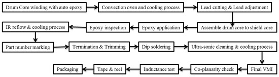
Figure 1.
Workstations to produce the inductor component.
The inductor component is examined and evaluated at all workstations in accordance with the requirements indicated in Table 1. There are 12 conditions with either a good or a bad outcome.

Table 1.
Good and bad conditions of electronic component.
These conditions are then translated into seven parameters such as wire condition, winding condition, epoxy condition, core condition, lead part condition, marking condition, and soldering condition. These parameters are classified into two types known as numerical and category data. The numerical data show that the observations can be analysed, whereas the categorical data show that they can be calculated. This approach, unfortunately, is limited to categorical data. As indicated in Table 2, all seven parameters are categorized as categorical data. Reséndiz-Flores et al. discussed that the normal scale is lower than the abnormal scale because the average MD for the normal group is near to 1.0, but the MD for the abnormal group is high [24].
Table 2.
Scales and conditions of normal and abnormal factors.
3.2. MTS under Teshima Using RT-Method
Pattern recognition is the emphasis of this approach. As indicated in Equation (1), the average value for each parameter was determined from the number of samples of the unit data.
Equations (2) and (3) are used to calculate the linear equation L and effective divider r respectively, for each unit data.
Furthermore, the sensitivity β is shown in Equation (4). β indicates the steepness of incline of the straight line. Ascending the line to the right indicates that the L is positive, whereas descending the line to the right indicates that the L is negative.
The total variation, variation of proportional term, error variation and error variance were calculated first as shown in Equations (5)–(7) and Equation (8) respectively.
Eventually, Equation (9) shows how to find the standard SN ratio η. The larger the value of η, the stronger will the relationship between input and output.
Equations (12) and (13) show the average of Y1 and Y2 for prediction of unit data origin.
Hence, Mahalanobis Distance (MD) for unit data is calculated based on Equation (14). MD always has a zero or a positive value, since A is non-negative definite.
For the signal data, linear equation L and effective divider r are calculated first as shown in Equations (15) and (16) respectively, for each sample. Note that, the average value of parameters and r is exactly from the unit data.
Then, Equation (17) shows equation of sensitivity β. The value of β is calculated for each signal data.
Moreover, Equations (18)–(21) are used to compute the total variation, variation of proportional term, error variation and error variance respectively.
Finally, the standard SN ratio ƞ is given as the following Equation (22). The larger the value of SN ratio η the stronger the relationship between input and output.
By using sensitivity β and standard SN ratio ƞ belonging to signal data, the two variables Y1 and Y2 are calculated for plotting in the scatter diagram. For Y1, β was used directly as shown in Equation (10), while Y2 will first was converted as follows to allow an evaluation of any scatter from the standard conditions as shown in Equation (11). Similarly, using Equations (12) and (13) shows the average of Y1 and Y2 for each signal data to predict their origin. Finally, MD can be calculated based on Equation (14).
3.3. MTS under Teshima Using T Method-1
MTS under Teshima using the T Method-1 is primarily concerned with parameter assessment. By creating a histogram, it can be confirmed that the data are normal or heavily occupied in the medium range. The highest sample was designated as unit data, while the remaining samples were designated as signal data. The average value for each parameter and the average value of output may be calculated using the number of samples in the unit data, as indicated in Equations (23) and (24).
The remaining unit data samples were classified as signal data. All data utilized to calculate the proportional coefficient β and SN ratio η were referred to as signal data. The average value of parameters and output pertaining to the unit data were then used to normalize the signal data. The goal of normalization is to make data extra adaptable by removing duplication. Normalization was carried out using Equations (25) and (26).
The proportional coefficient β and SN ratio η were calculated for each parameter as shown in Equations (27)–(33).
A positive value of β indicates that the steepness is ascending to the right whereas a negative value of β indicates that the steepness is descending to the right. The value of η should be positive, but if it is negative, it automatically turns to zero, meaning that the relationship between input and output is no longer significant. An integrated result is obtained by weighting it with SNR, which is the estimated measure of precision of each parameter. Thus, the integrated estimated value of the signal data can be calculated as Equation (34).
The integrated estimate SN ratio was computed using the following Equations (35)–(41). In fact, the SNR of integrated estimate value should be based on the suitability of OA.
where:
The relative relevance of a parameter was determined by examining how much the integrated estimate SN ratio starts to deteriorate whenever the item is not utilized. A two-level orthogonal array was adopted for evaluation. The application of an orthogonal array enables a comparison of the SN ratio of the integrated estimate under different situations. The orthogonal array’s two levels indicate that level 1 is the item that will be utilized and level 2 is the item that will not be used. In terms of the integrated estimate value’s SN ratio, the difference between the averages of SN ratio for level 1 and level 2 parameter by parameter is used to establish the relative significance of the items. With respect to the factorial effect graph, descending the line from left to right indicates that the parameter had an effect of elevating the output, or the parameter was defined as critical. Otherwise, ascending the line from left to right indicates that the parameter had an effect of lowering the output or the parameter was defined as non-critical.
With respect to the TDABC methodology, the first step in evaluating capacity utilization and unused capacity in a manufacturing setting is to identify activities and sub-activities that are important to the product. There are 16 workstations reflecting the primary activity and 49 sub-activities in this work. The general ledger was referred to discover the cost of resources provided, such as labour, machinery maintenance, raw materials, and consumables. The total number of working hours in a year was calculated to assess practical capacity. The company’s current hours of operation are Monday to Saturday, 7.30 a.m. to 5.30 p.m. The capacity cost rate in RM per minute was determined using Equation (42).
Furthermore, as demonstrated in Equation (43), the time equation was formulated. The more complicated the equation, the more accurate the capacity utilization and unused capacity.
where:
the time needed to perform an activity (minute)
the standard time to perform the basic activity (minute)
the estimated time to perform the incremental activity (minute)
the quantity of the incremental activity (time)
The estimation time for the sub-activity is the continuity from the primary activity to the sub-activity via several observations on the operators. The required capacity for a sub-activity is therefore evaluated by determining the amount of the activity in a month. The capacity utilization is further determined in terms of both cost and time. Lastly, the unused capacity of time is calculated by subtracting the value of practical capacity from used time, and the unused capacity of cost is derived when unused time is being multiply with the cost rate of capacity.
4. Results and Discussions
4.1. System Integration
System integration is the process of combining many independent subsystems or sub-components into one bigger system that allows the subsystems to work together. The symbiotic relationship formed by system integration enables the main system to accomplish the organization’s overall functionality. To demonstrate that the suggested solution is superior to others, it needs to be contrasted to all other system integrations. In terms of quality, this work employed a traditional method based on a control chart and MTS. This effort, considered ABC and TDABC in terms of expense. This study also demonstrated the possibility of system integrations by integrating a quality technique with a cost method, as seen in Figure 2.
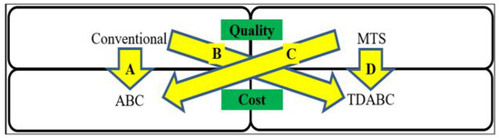
Figure 2.
System integrations.
Integration A is the interaction between the conventional and ABC systems. The electronic company is now using this integration to determine the cost per unit of goods. The traditional approach considered that all parameters were equally important, and will be replaced by the ABC system, which focuses on the cost driver, as indicated in Table 3. As a result, the cost of an inductor component adopting integration A is RM 1.58 per unit.
Table 3.
Costing structure under integration A.
Integration B is the interaction between the conventional and TDABC systems. The traditional approach assumed that all characteristics were equally relevant, and will be replaced by the TDABC system, particularly highlighting the capacity cost rate and time equation as illustrated in Table 4. As a result, the cost of an inductor component applying integration B is RM 1.67 per unit.
Table 4.
Costing structure under integration B.
Integration C is the interaction between the MTS and ABC systems. The MTS system suggested that parameters 1 and 2 had an impact on workstations 1, 2, 3, and 12. Workstations 5, 6, 7, and 12 were affected by parameter 3. Workstations 4, 5, 6, 7, 8, and 12 were impacted by parameter 4. Workstations 1, 2, 3, 4, 8, and 12 were affected by parameters 5 and 6. Workstations 10, 11, and 12 were impacted by parameter 7. As stated in Table 5, all of those parameters are substituted into the ABC system with an emphasis on the cost driver. As a result, the cost of an inductor component applying integration C is RM 0.80 per unit.
Table 5.
Costing structure under integration C.
Lastly, integration D is the interaction between the MTS and TDABC systems. The MTS system suggested that parameters 1 and 2 had an impact on workstations 1, 2, 3, and 12. Workstations 5, 6, 7, and 12 were affected by parameter 3. Workstations 4, 5, 6, 7, 8, and 12 were affected by parameter 4. Workstations 1, 2, 3, 4, 8, and 12 were affected by parameters 5 and 6. Workstations 10, 11, and 12 were affected by parameter 7. As stated in Table 6, all of those parameters are substituted into the TDABC system, which focuses on the capacity cost rate and time equation. As a result of employing integration D, the cost per unit of inductor component is RM 0.76.
Table 6.
Costing structure under integration D.
4.2. Significant Contribution of MTS to the Final Cost
To ensure that MTS and TDABC make a substantial contribution to the final cost, a comparison of integration types must be performed, as indicated in Table 7. To have an understanding of the benefits of MTS, the initial comparison was done between integration A and C, where conventional and MTS are compared while ABC was fixed. This demonstrated that the cost through integration C was lower than the cost through integration A because the MTS considers the degree of contribution for each parameter that impacts the increment or decrement to the final cost, whilst the conventional implies all parameters influence the final cost equally. Likewise, integration D was slightly less costly than integration B.
Table 7.
Cost through multiple integrations.
To reap the benefits of TDABC, a second comparison was done between integration A and B, in which ABC and TDABC were compared while conventional is fixed. This demonstrated that the cost through integration B was less expensive than the cost through integration A. This is because TDABC develops capacity cost rates from the associated costs of capacity provided and time equations with high flexibility that impacts the increment or decrement to the final cost, whereas ABC only has cost drivers to influence the final cost. Consequently, integration D was less expensive than integration C.
The final comparison was done between integration A and integration D to approach the benefits of MTS and TDABC. Integration A is the electronic company’s system, whereas integration D is the recommended solution or the key contribution of this work in the manufacturing environment. This demonstrates that the cost through integration D is less expensive than the cost through integration A because the MTS takes into account the degree of contribution for each parameter that impacts the increment or decrement to the final cost, whereas the TDABC develops capacity cost rate from related cost of capacity supplied and time equations with high flexibility that also affects the increment or decrement to the final cost. This discovery is validated by Kamil et al., and showed that the cost of a magnetic component using integration D was less than that of integration A [25].
As a result, this study concluded that integration D is the ideal approach to be implemented in the production setting compared to others.
5. Conclusions
Using MTS, this work evaluated the classification and degree of contribution of parameters in a manufacturing context. In the scatter diagram, healthy and unhealthy groups were displayed to show the distance between rejected and accepted components. Remarkably, neither group was alike and had a positive correlation. This work, on the contrary, assessed the degree of contribution for every parameter. Positive degree of contribution implies that the usage of parameter results in an increase in MD output, whilst negative degree of contribution means that the use of parameter results in a decrease in MD output. To achieve a lower MD, or to be closer to the healthy group, the positive degree of contribution must be reduced while the negative degree of contribution must be increased.
Applying TDABC, this work also examined the used and unused capacity in a production environment. For capacity utilization, three clusters were discovered. Type I, which is the workstation that over-utilized the provided apportionment, Type II which is the workstation that utilized a small portion of the provided apportionment, and Type III which is the workstation that largely utilized the provided apportionment. So, Type III is clearly the most significant, since management constantly sets the expenditure to reach a specific yearly production. Management could more precisely forecast their resources and costs in the future by recognizing the unused capacity of time and cost.
This study also presented the latest system integration of quality and cost in the manufacturing environment. Integration A (conventional-ABC), Integration B (conventional-TDABC), Integration C (MTS-ABC), and Integration D (MTS-TDABC) are the four types of integration addressed in this work. In a nutshell, Integration D is the right choice to be applied in the production environment. This is because MTS considers the degree of contribution for each parameter that impacts the increment or decrement to the final cost, and TDABC determines capacity cost rate from the related cost of capacity provided and time equations with high flexibility to determine the product’s complexity.
Author Contributions
Conceptualization, A.S.A.G.; Writing–original draft, F.L.M.S.; Writing–review & editing, S.N.A.M.Z.; Supervision, M.Y.A.; Funding acquisition, N.N.J. All authors have read and agreed to the published version of the manuscript.
Funding
The authors would like to thank the Malaysian Ministry of Higher Education for providing financial support under Fundamental Research Grant Scheme (FRGS) No. FRGS/1/2022/TK0/UMP/03/7 (University reference RDU220104).
Institutional Review Board Statement
Not applicable.
Informed Consent Statement
Informed consent was obtained from all subjects involved in the study.
Data Availability Statement
The datasets generated during and/or analysed during the current study are available from the corresponding author on reasonable request.
Conflicts of Interest
The authors declare no conflict of interest.
References
- Pourmehdi, M.; Paydar, M.M.; Ghadimi, P.; Azadnia, A.H. Analysis and Evaluation of Challenges in the Integration of Industry 4.0 and Sustainable Steel Reverse Logistics Network. Comput. Ind. Eng. 2022, 163, 107815. [Google Scholar] [CrossRef]
- Gajek, A.; Fabiano, B.; Laurent, A.; Jensen, N. Process safety education of future employee 4.0 in Industry 4.0. J. Loss Prev. Process Ind. 2022, 75, 104691. [Google Scholar] [CrossRef]
- Schwab, K. The Fourth Industrial Revolution, What It Means and How to Respond. Available online: https://www.weforum.org/agenda/2016/01/the-fourth-industrial-revolution-what-it-means-and-how- (accessed on 20 November 2022).
- Thames, L.; Schaefer, D. Software-defined Cloud Manufacturing for Industry 4.0. Procedia CIRP 2016, 52, 12–17. [Google Scholar] [CrossRef]
- Xu, G.; Song, Z. Performance analysis of a UAV-Assisted RF/FSO relaying systems for Internet of Vehicles. IEEE Internet Things J. 2022, 9, 5730–5741. [Google Scholar] [CrossRef]
- Chang, Z.P.; Li, Y.W.; Fatima, N.A. Theoretical survey on Mahalanobis-Taguchi system. Measurement 2019, 136, 501–510. [Google Scholar] [CrossRef]
- Jobi-Taiwo, A.A. Data Classification and Forecasting Using the Mahalanobis-Taguchi Method. Master’s Thesis, Missouri University of Science and Technology, Rolla, MO, USA, 2014. [Google Scholar]
- Xiao, X.; Fu, D.; Shi, Y.; Wen, J. Optimized Mahalanobis-Taguchi System for High-Dimensional Small Sample Data Classification. Comput. Intell. Neurosci. 2020, 2020, 4609423. [Google Scholar] [CrossRef]
- Sembiring, M.T.; Wahyuni, D.; Sinaga, T.S.; Silaban, A. Study of activity based costing implementation for palm oil production using value-added and non-value-added activity consideration in PT XYZ palm oil mill. In IOP Conference Series: Materials Science and Engineering (TALENTA-CEST 2017), Sumatera Utara, Indonesia, 7–8 September 2017; IOP Publishing: Bristol, UK, 2017. [Google Scholar]
- Bagherpour, M.; Nia, A.K.; Sharifian, M.; Mazdeh, M.M. Time-driven activity-based costing in a production planning environment. Proc. Inst. Mech. Eng. Part B J. Eng. Manuf. 2012, 227, 333–337. [Google Scholar] [CrossRef]
- Kont, K.R.; Jantson, S. Activity-based costing (ABC) and time-driven activity-based costing (TDABC): Applicable methods for university libraries. Evid. Based Libr. Inf. Pract. 2011, 6, 107–118. [Google Scholar] [CrossRef]
- Bokrantz, J.; Skoogh, A.; Berlin, C.; Wuest, T.; Stahre, J. Smart Maintenance: A research agenda for industrial maintenance management. Int. J. Prod. Econ. 2020, 224, 107547. [Google Scholar] [CrossRef]
- Ketkar, M.; Vaidya, O. Developing Ordering Policy based on Multiple Inventory Classification Schemes. Procedia Soc. Behav. Sci. 2014, 133, 180–188. [Google Scholar] [CrossRef]
- Abu, M.Y.; Jamaludin, K.R.; Shaharoun, A.M.; Sari, E. Pattern recognition on remanufacturing automotive component as support decision making using Mahalanobis-Taguchi System. Procedia CIRP 2015, 26, 258–263. [Google Scholar]
- Mota-Gutierrez, C.G.; Reséndiz-Flores, E.O.; Reyes-Carloset, Y.I. Mahalanobis-Taguchi system: State of the art. Int. J. Qual. Reliab. Manag. 2018, 35, 596–613. [Google Scholar] [CrossRef]
- Das, P.; Datta, S. Developing an unsupervised classification algorithm for characterization of steel properties. Int. J. Qual. Reliab. Manag. 2012, 29, 368–383. [Google Scholar] [CrossRef]
- Wang, N.; Zhang, Z. Feature recognition and selection method of the equipment state based on improved Mahalanobis-Taguchi System. J. Shanghai Jiaotong Univ. (Sci.) 2020, 25, 214–222. [Google Scholar] [CrossRef]
- Bose, S.; SahaRay, R.; Bandyopadhyay, R. Mahalanobis Taguchi System (MTS) and Mahalanobis Taguchi Gram-Schmidt (MTGS) methods as multivariate classification tools. Int. J. Ind. Syst. Eng. 2014, 16, 102–119. [Google Scholar] [CrossRef]
- Kaplan, R.S.; Anderson, S.R. Time-Driven Activity-Based Costing: A Simpler and More Powerful Path to Higher Profits; Harvard Business School Press: Boston, MA, USA, 2007. [Google Scholar]
- Medeiros, H.S.; Santana, A.F.B.; Guimarães, L.S. The use of costing methods in lean manufacturing industries: A literature review. Gestão Produção 2017, 24, 395–406. [Google Scholar] [CrossRef]
- Kaplan, R.S.; Anderson, S.R. Time-driven activity-based costing. Harv. Bus. Rev. 2004, 82, 131–138. [Google Scholar] [CrossRef]
- Gonzalez, M.; Nachtmann, H.; Pohl, E. Time-driven activity-based costing for healthcare provider supply chains. Eng. Econ. 2016, 62, 161–179. [Google Scholar] [CrossRef]
- MortajiIra, S.T.H.; Bagherpour, M.; Mazdeh, M.M. Fuzzy Time-Driven Activity-Based Costing. Eng. Manag. J. 2013, 25, 63–73. [Google Scholar] [CrossRef]
- Reséndiz-Flores, E.O.; Navarro-Acosta, J.A.; Mota-Gutiérrez, C.G.; Reyes-Carlos, Y.I. Fault detection and optimal feature selection in automobile motor-head machining process. Int. J. Adv. Manuf. Technol. 2018, 94, 2613–2622. [Google Scholar] [CrossRef]
- Kamil, N.N.N.M.; Zaini, S.N.A.M.; Abu, M.Y. A Case Study on the Un-Used Capacity Assessment Using Time Driven Activity Based Costing for Magnetic Components. Int. J. Ind. Manag. 2021, 9, 32–53. [Google Scholar] [CrossRef]


Disclaimer/Publisher’s Note: The statements, opinions and data contained in all publications are solely those of the individual author(s) and contributor(s) and not of MDPI and/or the editor(s). MDPI and/or the editor(s) disclaim responsibility for any injury to people or property resulting from any ideas, methods, instructions or products referred to in the content. |
© 2023 by the authors. Licensee MDPI, Basel, Switzerland. This article is an open access article distributed under the terms and conditions of the Creative Commons Attribution (CC BY) license (https://creativecommons.org/licenses/by/4.0/).