Abstract
Students’ mental health has always been the focus of social attention, and mental health prediction can be regarded as a time-series classification task. In this paper, an informer network based on a two-stream structure (TSIN) is proposed to calculate the interdependence between students’ behaviors and the trend of time cycle, and the intermediate features are integrated layer by layer to realize the prediction of mental health by a gating mechanism. Through experiments on a real campus environment dataset (STU) and an open dataset (MTS), it is verified that the proposed algorithm can obtain higher accuracy than existing methods.
1. Introduction
The mental health problems of students have been widely and highly concerned by schools and society. In recent years, there has been an increase in cases of student mental health problems which affect their grades and lead to drop out or even suicide [1]. The State Education Commission conducted psychological tests and investigations on 126,000 college students, and the results showed that 20.23% of those students had obvious psychological problems [2]. Therefore, it is hoped that by predicting the mental health status of students, finding students with mental abnormalities in advance, and allowing schools and teachers to intervene psychologically with students, the occurrence of malignant events could be reduced and tragedy could be avoided.
Most of the existing methods are based on qualitative research, which use questionnaires and self-evaluations to obtain and analyze students’ mental health data. Because many students are reluctant to reveal their true psychological conditions, strong subjectivity is often present in the research results. At the same time, the small sample size and lack of comprehensive data may also lead to inaccurate and unreliable conclusions.
The main goal of this paper is to associate students’ daily behaviors with their psychological conditions by combining qualitative and quantitative research methods, extract effective information from massive data generated by students’ daily lives at school, identify and predict students’ psychological conditions through analysis and mining, and find students with psychological abnormalities.
With the development of campus intellectualization and digitalization, a large amount of behavioral data (e.g., meals, travel, study and Internet access) are collected. On the basis of these data, this paper proposes a TSIN network based on a two-stream informer, with captures the interdependence between students’ behaviors and the trend of time cycle through the two-stream structure, and integrates the intermediate features layer by layer. Finally, a gating mechanism is used for classification prediction. The main contributions of this paper are summarized as follows:
- An architecture based on a two-stream informer is designed. The Time Encoder and Behavior Encoder are used to capture the interdependence between students’ behaviors and the time cycle trend, respectively;
- In order to prevent information loss, the features of the two channels are fused using an Intermediate Fusion Module;
- A dataset with 8213 students’ behavioral data is made for experimental analysis; the TSIN is evaluated on this dataset and 11 multivariate time-series benchmark datasets, and a comprehensive ablation study is conducted with other advanced deep learning models. The experiments show that the TSIN has good performance.
2. Related Work
2.1. Education Data Mining
In recent years, data mining technologies have been used to analyze and mine data generated by students at school with remarkable results, and the results of data mining have been widely applied in education and teaching [3]. These studies analyzed students’ activity habits [4,5,6] and consumption behavior [7,8,9], explored the relationship between students’ activities and grades [10,11], explored poor students [12,13], etc. Yao et al. [14] collected students’ campus behavior data, designed a prediction framework for academic performance based on multi-task learning ranking, and experimentally found that student characteristics such as diligence and regularity were closely related to academic performance. Govindasamy et al. [15] predicted the final grades of students in four private universities through various classification and clustering algorithms in a data mining study. Li et al. [16] applied a KMeans clustering algorithm to students’ consumption behavior, and used an Apriori algorithm to explore the correlation between students’ consumption behavior and consumption performance. Morelli et al. [17] conducted a questionnaire survey and characterized four university freshman dormitories to study the role of student happiness and empathy on interpersonal relationships, and to mine and analyze students’ social networks. Ding et al. [18] designed a KMeans clustering algorithm based on density division and applied it on the Spark framework to divide students into different groups and formulate corresponding management methods for each group.
The state of students’ mental health has been a problem that cannot be ignored, and many experts and scholars have analyzed and researched this issue and proposed related methods. Chen and Jiang [19], in the context of the current situation of college students’ mental health education, analyzed the factors affecting mental health education through cognitive calculation. They found that students’ daily lifestyles were positively correlated with mental health, and proposed corresponding solutions. Pedrelli et al. [20], through the universality and treatment of students’ psychology and spirit, understood the developmental stages of students’ psychological abnormalities and the uniqueness of their environment, and described the persistence of college students’ mental health problems and their influencing factors. Hokanson et al. [21] conducted a 9-month survey on inter-personal relationships and other life factors of students with mental problems, and found that students with mental abnormalities had less communication with others, tended to ignore the friendly behaviors of others and suffered higher pressure in daily life and learning processes. These investigations and studies on students’ mental health provide clear research ideas for the study of students with psychological abnormalities in this paper.
In summary, researchers have analyzed students’ academic performance and social relations, and aimed to identify students with deficits through different dimensions of data and different methods, explored the correlation between students’ behavior and their mental health and found students with psychological abnormalities with the aim to provide timely psychological counseling and intervention.
2.2. Time-Series Classification
The recognition and prediction of students with mental health abnormalities can be regarded as a time-series classification problem. Time-series classification methods based on machine learning and deep learning are currently the mainstream time-series classification methods [22,23].
Some early methods adopted machine learning classifiers, and can achieve satisfactory results in some specific domains [22]. Jalalian et al. [24] constructed a classifier, GDTW-P-SVMs, with variable-length input sequences; the DTW method was used to convert the native time series into feature vectors, which were then used as the input to the SVM model. Yamada et al. [25] proposed a split detection method for decision tree induction by exhaustively searching for the optimal time series in the data. Gupta et al. [26] proposed an early multivariate time-series classification method using a Gaussian process learning method to estimate the minimum length required by the time series to help construct an integrated classifier with expected accuracy.
In recent years, methods based on deep learning have been widely used in various domains, including sequential classification tasks. Wang et al. [27] proposed a Multilayer Perceptron (MLP), whose structure consists of multiple fully connected layers, each of which is followed by a ReLU activation function and finally a Softmax classifier. Wang et al. [27] proposed a Fully Convolutional Network (FCN). Different from previous convolution, FCN uses Global Average Pooling (GAP) to replace the final full connection layer, which can not only reduce the number of parameters, but also improve the experimental accuracy. Wang et al. [27] proposed a Residual Network (ResNet) to solve the problem of gradient disappearance in the process of deepening layers through residual links. Cui et al. [28] proposed a Multi-scale Convolutional Neural Network (MCNN) which uses multiple branches for transformation to obtain features of different frequencies and time scales, and outputs them through two convolutional layers—a fully connected layer and finally a Softmax layer. Yi et al. [29] proposed a Multi-Channel Deep Convolutional Neural Network (MCDCNN) that automatically learns the features of a single univariate time series in each channel, then combines the output of all channels into the feature representation of the last layer and finally connects it to the MLP layer for classification. Tanisaro et al. [30] modified the Time Warping Invariant Echo State Network (TWIESN) applied to time-series prediction and applied it to time-series classification. Fazle et al. [31] proposed the LSTM-FCN model, where the time series were respectively passed through LSTM and FCN, and then the data obtained from the two channels were splintered for the final classification prediction. Liu et al. [32] introduced a Transformer model into time-series classification and built a two-tower structure to code time features and channel features, respectively. The model can visualize the features learned by the model, and has certain interpretability.
3. Proposed Method
3.1. Problem Description
The research objective is to identify students’ mental health status according to a dataset of students’ daily behaviors. The daily behavior data of the students is measured in weeks. In a given week, the daily behavior data of students , and the daily behavior data of all students form a dataset . The students’ mental health status was divided into two categories: mental health status , where indicated that the students’ mental health status was normal and indicated that the students’ mental health status was abnormal.
3.2. Overview of the Framework
As shown in Figure 1, the network structure based on the two-stream informer is divided into three layers: input layer, encoding layer and classification prediction layer. The input layer makes data embedding and location coding for the original data. In the encoding layer, a Time Encoder and Behavior Encoder based on multiple attention were designed to extract each embedded feature, and the features of the two encoders were fused using the Intermediate Fusion Module. The classification prediction layer uses a gating mechanism to classify and predict students’ mental health status.
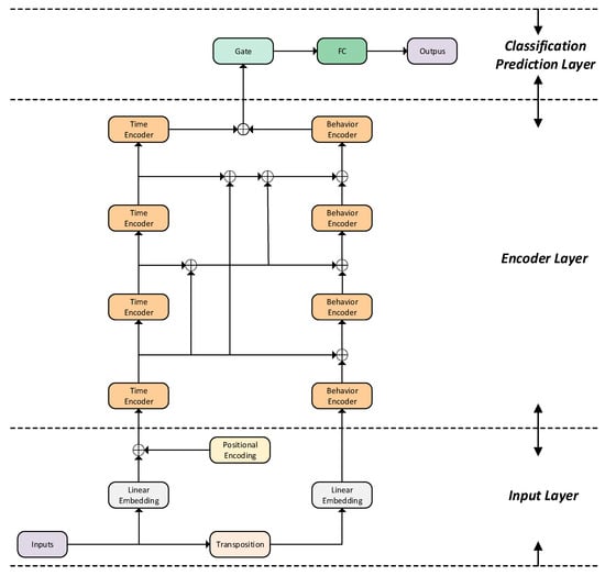
Figure 1.
Model architecture of the two-stream informer network.
3.3. Input Layer
The data input layer model requires the data input of dimension, so the input data need to be embedded; that is, the full connection layer is used to convert the feature dimension of the input data into the dimension. Meanwhile, since it is difficult for the self-attention mechanism to capture the position relation in the time series, a position coding needs to be added to the Time Encoder [33], as shown in Equation (1):
is the Time Encoder position coding value; represents the position information of the embedded vector and represents the index of each value belonging to the embedded vector.
3.4. Encoding Layer
In the encoding layer, a new backbone network is proposed that is composed of the Time Encoder, Behavior Encoder and its Intermediate Fusion Module. The Time Encoder extracts the sequence feature information from the time dimension and uses the informer encoder using a mask to obtain the time cycle trend. The Behavior Encoder extracts the behavior feature information from the behavior dimension and uses the informer encoder to obtain the behavior dependency. In the Intermediate Fusion Module, the features extracted by each Time Encoder and the features extracted by the Behavior Encoder are fused, and then a convolution layer with convolution kernel of 1 is passed through. After the whole process is repeated four times, the encoder features of the two channels are fused as the output of the backbone network.
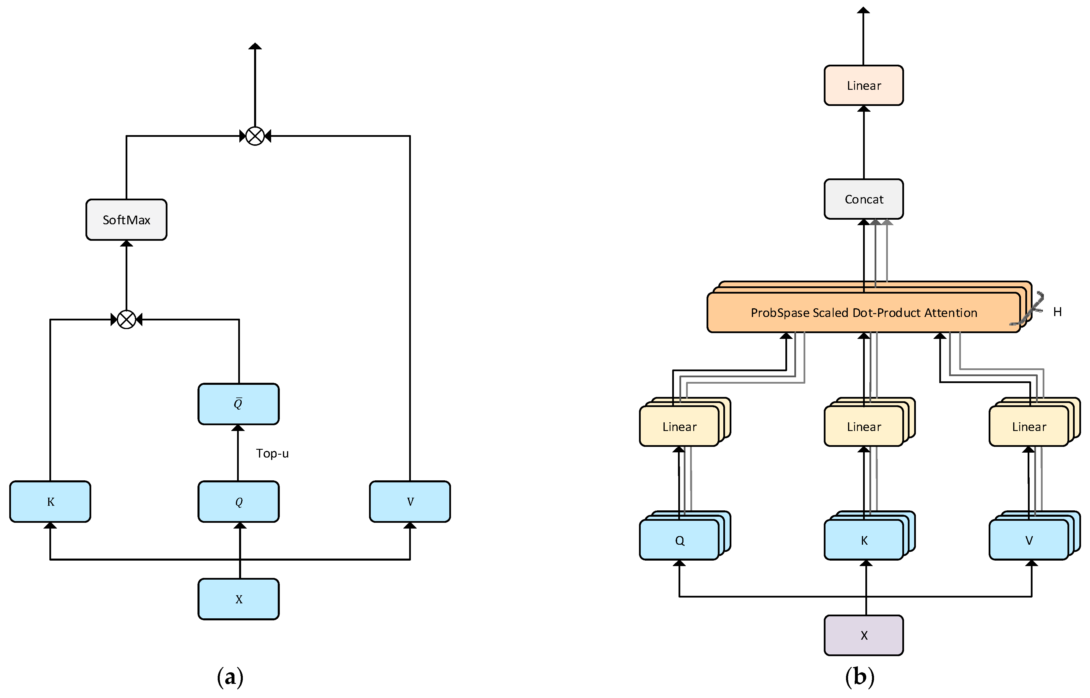
The key part of the Time Encoder and Behavior Encoder is the self-attention module. ProbSparse self-attention [34] is a kind of improved self-attention that can reduce the quadratic computational complexity of the self-attention mechanism and solve the classification prediction problem of long sequence data. Its overall architecture is shown in Figure 2a.
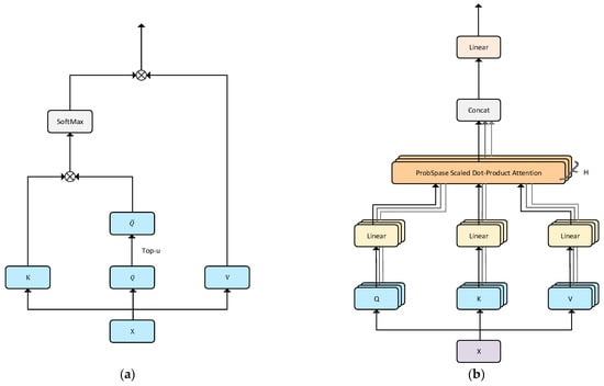
Figure 2.
(a) ProbSparse self-attention; (b) multi-head attention layer.
In the following, , and respectively represent the -th line in , and . According to the equation of Tsai et al. [35], the attention of the -th query is defined as a kernel smoother in probabilistic form:
According to probability to combine values and obtain the final output,
Based on the long tail property, the key part is to calculate the distance between the probability distribution and the discrete uniform distribution of the query and key dot product pairs, so as to screen out the dominant dot product pairs. The Kullback–Leibler divergence attention is used to calculate the probability distribution with uniform distribution similarity.
If the case of -th query increases , its probability distribution and attention should be more diverse, and have a higher probability in the long tail distribution header fields contained in the edge of the dot product. For each value, only the leading query of top- is selected:
where is a sparse matrix containing only queries.
Compared with single-head self-attention, multi-head self-attention can capture different information through different projection spaces, which enhances the feature extraction ability of the encoder. The structure of multiple self-attention layers is shown in Figure 2b. It is sent to each self-attention layer through a linear projection. The information obtained from the model input via linear projection is sent to the attention layer with the following output:
3.4.1. Time Encoder
Time-series features are captured by calculating paired attention weights between all time steps and using masked self-attention to focus at every point on all channels. Like the Transformer, masking ensures that the current output is only dependent on the previous input without time leakage. Therefore, attention encoders with masks can better capture time characteristics.
Frist, a subset of is selected from as the initial input of the Time Encoder,
where represents the input of the Time Encoder, and is the number of Time Encoder layers in the network.
Secondly, query matrix , key matrix and value matrix are obtained after linear transformation, and then processed by a ProbSparse self-attention layer.
is a time attention function applied to the time dimension, is a nonlinear activation function, which is processed by function in the model. , and are the behavior characteristic dimensions of query, key and value.
Finally, a two-layer feedforward neural network is used, and each sub-layer is normalized by one layer,
where represents the normalization of layer, and the results obtained in the previous step are added and normalized again.
The whole Time Encoder process is designed as Equation (10):
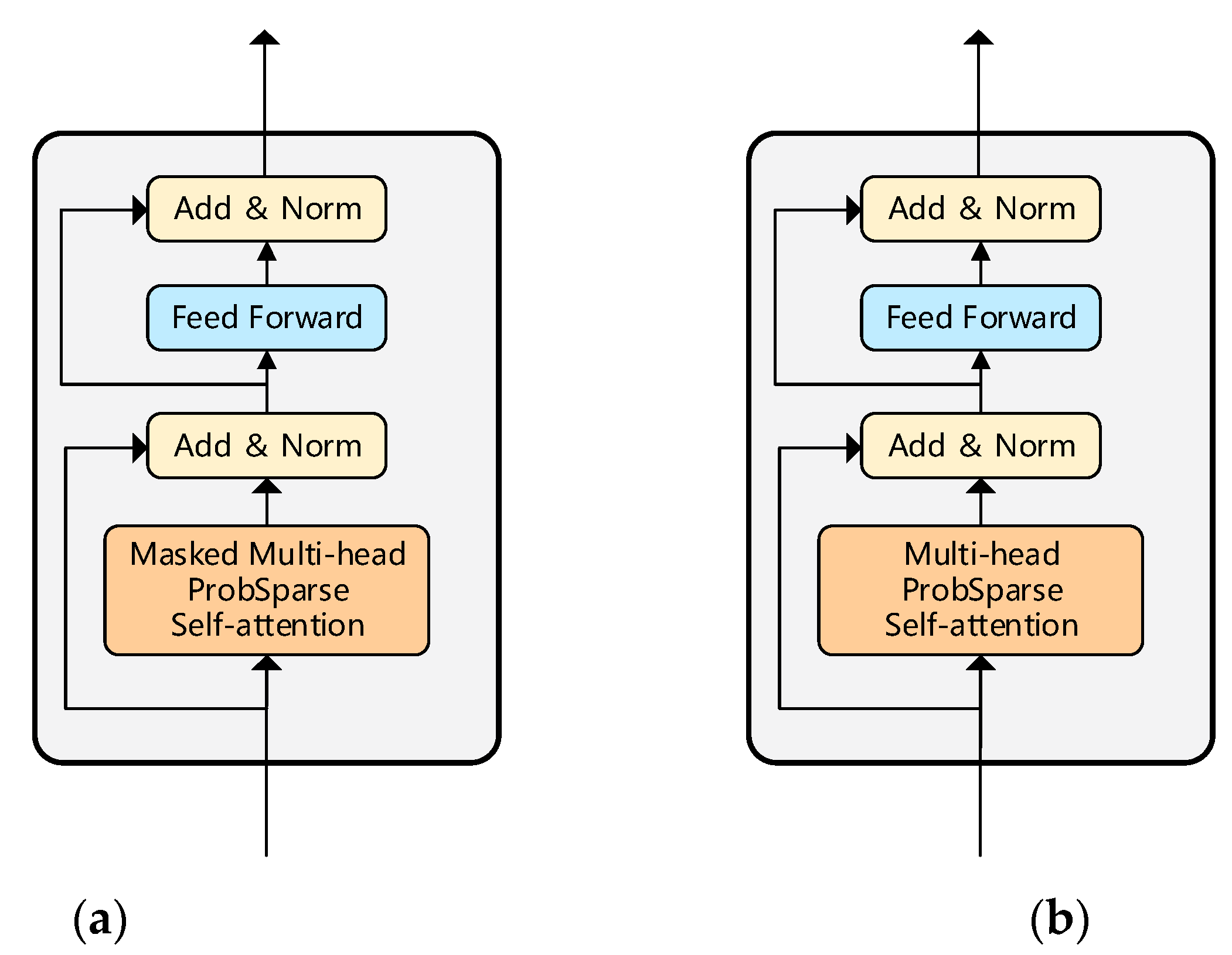
The resulting is fed to the next Time Encoder. There are four Time Encoders in the backbone network. The structure of the Time Encoder is shown in Figure 3a.

Figure 3.
(a) Time Encoder; (b) Behavior Encoder.
3.4.2. Behavior Encoder
The Behavior Encoder extracts the behavior information in the data by calculating the attention weights among different channels with all time steps.
First, select a subset of the transposed as input data,
where is the input of the Behavior Encoder, the first input is , obtained after transpose, the other inputs are the output fusion from the two encoders and is the number of Behavioral Encoder layers in the network.
Secondly, query matrix , key matrix and value matrix are obtained after linear transformation, and then after a ProbSparse self-attention layer processing.
where is the behavior attention function applied to the behavior dimension.
Finally, a two-layer feedforward neural network is used, and each sub-layer is normalized one layer at a time. In this step, the vectors before and after the previous step are added and normalized again.
The whole process design of the Behavioral Encoder is shown in Equation (13):
The resulting is fed to the next Behavior Encoder. There are four Behavior Encoders in the backbone network. The construction of the behavioral encoder is shown in Figure 3b.
3.5. Intermediate Fusion Module
If the data are processed in parallel between the Time Encoder and the Behavior Encoder, and the results obtained by the two encoders are ultimately merged, the information loss generally occurs when the number of encoder layers is large. In order to reduce the loss of information, a convolution layer with convolution kernel of 1 is adopted in the Intermediate Fusion Module to fuse the sequence information extracted by the Time Encoder with the dependence relationship extracted by the Behavior Encoder. Different from Cao et al. [36], in this paper, the temporal features extracted by the previous Time Encoder are fused with the behavioral features of the current Behavior Encoder in each layer to further reduce the impact caused by information loss.
3.6. Classification Prediction Module
After the of Time Encoder and of Behavior Encoder, the Gate Layer [32] method is used in the first step to adaptively fuse the two types of features, reconstruct the features and splice them into a vector, input them into fully connected layer and apply Softmax function for processing. The obtained feature-related gating weight is shown in Equation (14):
In the second step, the weighted vector is calculated and passed through a fully connected layer to obtain the final prediction probability vector y of students’ mental health as in Equation (15):
4. Experimental Results and Analysis
4.1. Basic Settings
4.1.1. Dataset
Two datasets, MTS and STU, were used for the evaluation. Table 1 shows the different characteristics of the MTS dataset and the STU dataset used in our experiment. The first dataset, MTS, is a subset of the public data set Baydogan [37], and contains 10 multivariate time-series datasets such as ArabicDigits and CharacterTrajectories. By default, all datasets are divided into training and testing parts, while aligning all time-series lengths and performing normalization. The second dataset, STU, comprises real campus data of a university in two semesters, in which weekly canteen consumption time, consumption times and consumption amounts of students were taken as consumption data. Weekly online times and online duration are used as online data; weekly waking time and rest time are used as daily routine data. We also obtained a dataset on students’ mental health status from the university’s counseling center, which contains 6127 general students and 2086 students whose mental health status requires focused attention.

Table 1.
The multivariate time-series classification archive.
4.1.2. Comparison Methods
We chose the following deep learning models as benchmarks:
- Fully Convolutional Network (FCN) and Residual Network (ResNet) [27], which are the best deep learning models in multivariate time-series classification tasks [23]. Multilayer Perception (MLP) also serves as a simple baseline.
- Universal Neural Network coder (Encoder) [38].
- Multi-scale Convolutional Neural Network (MCNN) [28].
- Multi-Channel Deep Convolutional Neural Network (MCDCNN) [29].
- Time Convolutional Neural Network (Time-CNN) [39].
- Time Le-Net (t-LeNet) [40].
- Time Warping Invariant Echo State Network (TWIESN) [30].
- Gated Transformer Network (GTN) for multivariate time-series classification [32].
4.1.3. Parameter Setup and Experimental Support
All experiments were run on ubuntu20.04 OS and supported by a server equipped with Intel(R) Xeon(R) Platinum 8255C@2.50GHz CPU and NVIDIA GeForce RTX 2080Ti 11GB GPU. Based on the Pytorch 1.11.0 framework, Python 3.8 was used to implement the TSIN model. The two-stream informer network was trained with Adagrad with learning rate 0.0008 and dropout 0.2. The classification cross entropy was used as the loss function. The training set and test set were tested every iteration for a certain number of times, and the best test results and their hyperparameters were recorded. For the fairness of comparison, the model with minimum training loss was selected for test accuracy [23].
4.1.4. Evaluation Metric
Following a common practice in temporal classification work [41], the accuracy (the proportion of correctly identified categories in all predictions) was used as a measure. The accuracy rate was calculated as in Equation (16):
4.2. Comparison with Representative Works
4.2.1. Accuracy Comparison
We evaluated the performance of the proposed TSIN model for timing classification tasks and proved the effectiveness of feature engineering based on the two-stream informer network.
The experimental results are shown in Table 2. The results were calculated using the TSIN model in the AUSLAN, CharacterTrajectories, Libras and Wafer data sets for the 10 datasets of MTS. Compared with the best results of the other 10 baselines, the results were improved by 0.50%, 0.20%, 0.55% and 0.55% in these datasets, respectively. The TSIN model had the best accuracy of 81.45% in the STU dataset, an improvement of 0.15% compared with the other best results. FCN had the highest accuracy of 98.77% for ArabicDigits and 91.84% for UWave out of 11 datasets; GTN with the same two-stream structure had the best accuracy of 98.38% on the JapaneseVowels dataset. On the CMUsubject16 dataset, both the TSIN model and the GTN model with the same two-stream structure achieved perfect accuracy.
Table 2.
Test accuracy of the TSIN and other benchmark models on the multivariate time-series dataset.
In addition, TCN, ResNet and Encoder also had high accuracy, and TCN and the TSIN had the highest accuracy of 87.00% on the ECG data set. At the same time, TCN, ResNet, Encoder, FCN and GTN also had the highest precision of 100.00% on the WalkvsRun data set alongside the TSIN. The success of ResNet is largely due to its deeply flexible architecture; the small number of filters in TCN is the main reason for its success on small datasets, but this shallow architecture cannot capture the variability of large time-series datasets efficiently modeled by the FCN and ResNet architectures. MLP also had good performance in multiple datasets because it contains enough connection layers to fit real-time trends.
The reason that MCDCNN did not have the highest accuracy on any dataset may be due to the use of a nonlinear FC layer instead of the GAP in FCN and ResNet—this FC layer reduces the effect of learning time-invariant features. Meanwhile, for the only TWIESN model in the experiment that uses a cyclic structure, the accuracy was poor in time series with longer time sequences, such as the AUSLAN, CMUsubject16, UWave and WalkvsRun datasets, and their predictions were all far from being able to compete with the best accuracy because the cyclic structure may lose some of the information that appears early in long time-series information.
The accuracy of the MCNN and t-LeNet architectures was very low, and they had the worst prediction accuracy of the eight datasets; both of these models augment the training data by extracting subsequences. Unlike models that classify from the entire subsequence, they learn features from shorter subsequences and finally assign labels to the time series using majority voting. The lower accuracy of these two methods suggests that this method of extracting subsequences from time series does not guarantee that features of the time series are not lost when they are segmented.
Overall, the results show that the proposed model TSIN was the best architecture with the highest accuracy achieved on the eight evaluated datasets, followed by FCN and GTN, both of which had the highest accuracy on three datasets. MCNN and t-LeNet, which partition the time series into subseries, had the worst prediction results.
4.2.2. Time Complexity Comparison
As the inspiration for our work, the most time-consuming part of the GTN is the two encoders. Since these two encoders can run in parallel, we can estimate the time complexity in one of the encoders. The encoder in the GTN consists of a multi-headed self-attentive layer. We assume that the input data dimension is , where is the sequence length and is the embedding dimension. Then, the time complexity of an attention layer can be estimated as , where is the time complexity of the multi-headed self-attention and is the time complexity of the linear mapping of input and output.
Similar to the estimation of the GTN, we attempt to estimate the time complexity of the TSIN encoder because we use ProbSparse self-attention to reduce the computational load. Since the query matrix in ProSparse self-attention includes only the top-u queries, under the control of a constant sampling factor , we set , and then we can estimate the time complexity of multi-headed self-attention in the encoder as . The time complexity of an attention layer can be estimated as .
4.3. Ablation Test
In order to study the performance gains of each module in the TSIN, a comprehensive ablation experiment was performed as shown in Table 3.
Table 3.
Ablation study of the Time Encoder, Behavior Encoder, Intermediate Fusion Module and gating in the TSIN.
The Behavior Encoder can capture the dependency between various behaviors, but Time Encoders cannot make good use of the advantages of multivariate time series. The processing method makes multivariate time series become like univariable time series, losing the connection between various features. Therefore, the effect of most Behavior Encoders is better than that of Time Encoders. The gating mechanism can integrate the features of the two channels well through adaptive weights. If the features encoded by the two encoders are simply connected, the accuracy of the prediction will be reduced to varying degrees.
Different time series data may have different propensities towards temporal and behavioral characteristics. For example, on the dataset UWave, models with only Time Encoders had superior performance to other models; on the ArabicDigits data set, with both Time Encoder and Behavior Encoders, the model without Intermediate Fusion Module had the highest accuracy.
4.4. Analysis of Attention Map
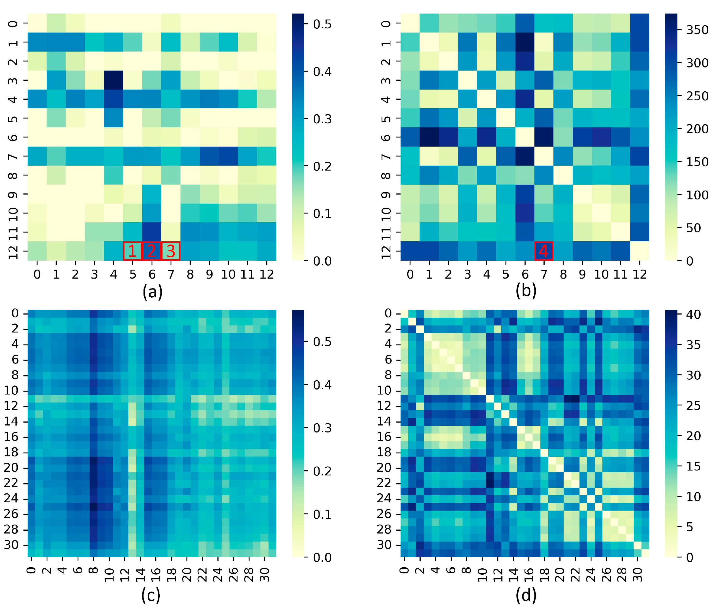
Note that the matrix represents the correlation of behavior and time steps, respectively. We selected a sample from the STU data set for visualization of both attention maps. Figure 4a analyzes the behavior-related attention graph and labels three blocks (b1–b3). For the attention diagram of the behavioral encoder, Figure 4b shows the calculation of the DTW distance of the time series on different channels and marks a block (b4). Figure 4c shows an analysis of the time-dependent attention graph, and Figure 4d shows the calculation of the Euclidean distance of different behaviors for each time step, since there is no timeline at the same point in time and thus DTW is not required. In Figure 5, the original time series for the corresponding channel is plotted. In the later analysis, channel12 is used for student break time (abbreviated c12).
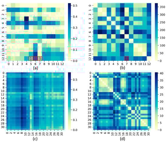
Figure 4.
(a) Time Encoder attention map (upper–left); (b) Time Encoder DTW (upper–right); (c) Behavior Encoder attention map (bottom–left); (d) Behavior Encoder L2 distance (bottom–right).
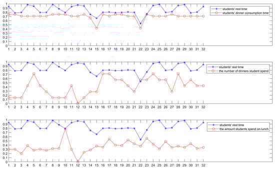
Figure 5.
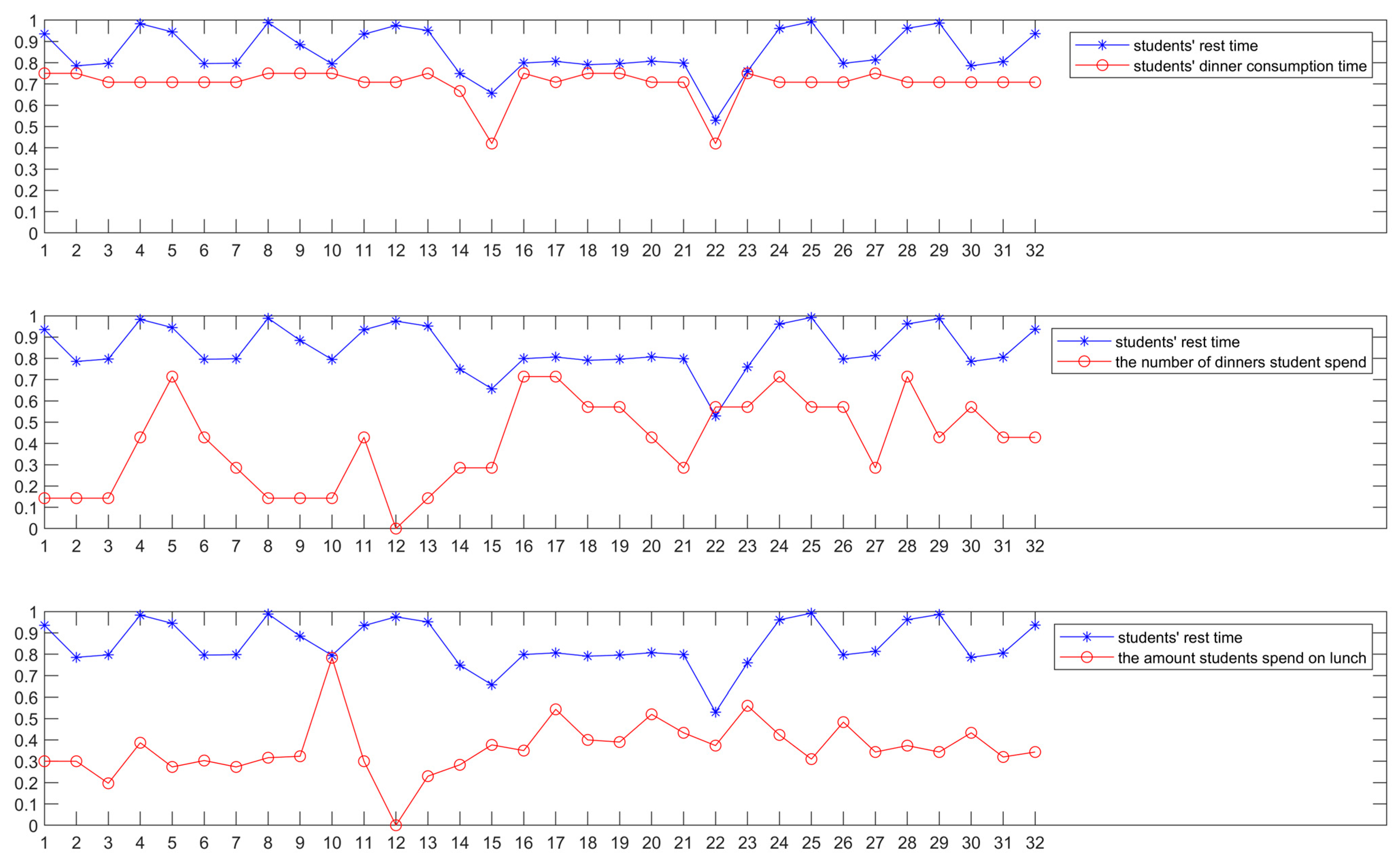
Drawing of the raw time series in different behavior pairs.
From Figure 4a, it can be seen that b2 has a relatively high attention score, that is, c6 (students’ dinner consumption time) is highly correlated with c12 (students’ rest time). From Figure 5, it can be clearly seen that c6 and c11 have relatively similar shapes and trends. b1 and b3 have lower attention scores. Both c5 (the amount students spend on lunch) and c7 (the amount students spend on dinners) show very different and even opposite trends compared to c12 (students’ rest time). It can be seen that the behavioral attention learned by the model from the time series can capture similar sequences, which work together to make the output of the model constantly fit the real label.
Figure 4b shows the DTW of the Time Encoder, where b4 represents a very small DTW distance between c5 and c12. However, it can be seen from Figure 5 that c12 and c5 are very different in both trend and shape, which indicates that the size of DTW distance matrix has little influence on the attention calculation of the Behavior Encoder. For the Behavior Encoder, since the correlation between behaviors is at the same time point, the special Euclidean distance of DTW at the same time point is used as the distance measure. Through the analysis of the behavioral attention diagram and the Euclidean distance matrix in Figure 4c,d, it is found that the distance and shape similarity between time series have an effect on the calculation of the attention fraction in the TSIN, but the effect is not obvious.
4.5. Analysis of Features
The behavioral characteristics consumption data (e.g., weekly canteen consumption times, consumption amount and consumption time), online data (e.g., weekly online time and online duration) and daily routine data (e.g., weekly wake up time and rest time) predict the mental health status, and the results are shown in Figure 6. The results show that these three behavior characteristics have a certain influence on students’ psychology. Among them, consumption data is the most effective, because it is the most accessible data among students. Compared with online data and daily routine data, the data of students’ consumption of three meals is the most frequently generated data in students’ daily lives. Moreover, it has a certain accuracy and can obtain higher prediction accuracy.
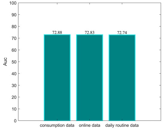
Figure 6.
Test accuracy of the TSIN on different student behavior sets.
At the same time, the accuracy of the daily routine data generated by students is low because, compared with the consumption data that can be recorded through the campus card and the online data that can be recorded through the campus network, the students’ daily wake up and work and rest data are not as easy to obtain and process. In this paper, among the first consumption time of the daily campus card, the first login time of the campus network, the time of punching in and other data, we chose the earliest one as the wake-up time. As rest time we chose the latest among the latest consumption time of the campus card, the latest logout time of the campus network and the time of punching in the early morning. In spite of this, there are still some deviations in the obtained daily routine data, which led to low prediction accuracy.
5. Conclusions
In view of the fact that most of the existing studies on predicting students’ mental health status use qualitative methods and do not adequately collect students’ relevant characteristics, this paper obtains students’ daily behavior data from three aspects (canteen consumption, Internet access and daily routine), and proposes an informer network based on a two-stream structure (TSIN) to analyze students’ daily behavior data to determine whether they need mental-health-focused attention for classification prediction. This model uses Time Encoder and Behavior Encoder to capture students’ time cycle trend and behavior dependence, respectively, prevents information loss through an Intermediate Fusion Module, and uses a gating mechanism for classification prediction. Experimenting with 10 multivariate time series from public datasets, the TSIN obtained the highest accuracy in seven experiments, and was able to obtain higher accuracy in predicting students’ mental health status compared to other time-series classification models, verifying the advantages of the model.
However, the experiments in this paper have the following disadvantages: (1) When collecting data from students, we only considered some of their behavioral data in daily life, while in real life students with abnormal mental health conditions often have their learning affected as well. (2) In making predictions about mental health status, we treated each student as an individual, and students with abnormal mental health status usually have some influence on those around them. In the future, we will try to collect more behavioral characteristics of students, especially in terms of student learning, including data related to the library and classrooms, to more comprehensively describe students’ daily behaviors. We will also use the graph structure to construct a network of relationships among students, and give higher weights to students who are closely related to students with abnormal mental health status in the model to improve the prediction accuracy. Since each student’s mental health status has abnormalities, we will try to let the model learn from psychologists’ ranking of the number of students’ psychological abnormalities so that schools and teachers can allocate resources more rationally and cover all students who need psychological counseling as much as possible.
Author Contributions
Conceptualization, X.D.; methodology, J.X.; validation, J.X.; formal analysis, J.X.; writing—original draft preparation, J.X.; writing—review and editing, X.D., H.K., C.X. and H.Z.; supervision, X.D. All authors have read and agreed to the published version of the manuscript.
Funding
This research received no external funding.
Institutional Review Board Statement
Not applicable.
Informed Consent Statement
Not applicable.
Data Availability Statement
Not applicable.
Conflicts of Interest
The authors declare no conflict of interest.
References and Notes
- Chu, Y.; Yin, X. Data Analysis of College Students’ Mental Health Based on Clustering Analysis Algorithm. Complexity 2021, 2021, 9996146. [Google Scholar] [CrossRef]
- Tang, Q.; Zhao, Y.; Wei, Y.; Jiang, L. Research on the mental health of college students based on fuzzy clustering algorithm. Secur. Commun. Netw. 2021, 2021, 3960559. [Google Scholar] [CrossRef]
- Baker, R. Data mining for education. Int. Encycl. Educ. 2010, 7, 112–118. [Google Scholar]
- Hsieh, K.Y.; Hsiao, R.C.; Yang, Y.H.; Lee, K.H.; Yen, C.F. Relationship between self-identity confusion and internet addiction among college students: The mediating effects of psychological inflexibility and experiential avoidance. Int. J. Environ. Res. Public Health 2019, 16, 3225. [Google Scholar] [CrossRef] [PubMed]
- Ding, Y.; Chen, X.; Fu, Q.; Zhong, S. A depression recognition method for college students using deep integrated support vector algorithm. IEEE Access 2020, 8, 75616–75629. [Google Scholar] [CrossRef]
- Akram, A.; Fu, C.; Li, Y.; Javed, M.Y.; Lin, R.; Jiang, Y.; Tang, Y. Predicting students’ academic procrastination in blended learning course using homework submission data. IEEE Access 2019, 7, 102487–102498. [Google Scholar] [CrossRef]
- Yang, Z.; Su, Z.; Liu, S.; Liu, Z.; Ke, W.; Zhao, L. Evolution features and behavior characters of friendship networks on campus life. Expert Syst. Appl. 2020, 158, 113519. [Google Scholar] [CrossRef]
- Wang, Y.; Wang, Q.W.; Tao, Y.Y.; Xie, W.W. Empirical Study of Consumption Behavior of College Students under the Influence of Internet-based Financing Services. Procedia Comput. Sci. 2021, 187, 152–157. [Google Scholar] [CrossRef]
- Lim, H.; Kim, S.; Chung, K.M.; Lee, K.; Kim, T.; Heo, J. Is college students’ trajectory associated with academic performance? Comput. Educ. 2022, 178, 104397. [Google Scholar] [CrossRef]
- Asif, R.; Merceron, A.; Ali, S.A.; Haider, N.G. Analyzing undergraduate students’ performance using educational data mining. Comput. Educ. 2017, 113, 177–194. [Google Scholar] [CrossRef]
- Su, Y.; Liu, Q.; Liu, Q.; Huang, Z.; Yin, Y.; Chen, E.; Ding, C.; Wei, S.; Hu, G. Exercise-enhanced sequential modeling for student performance prediction. In Proceedings of the AAAI Conference on Artificial Intelligence, New Orleans, LA, USA, 2–7 February 2018; Volume 32. [Google Scholar] [CrossRef]
- Wu, F.; Zheng, Q.; Tian, F.; Suo, Z.; Zhou, Y.; Chao, K.M.; Xu, M.; Shah, N.; Liu, J.; Li, F. Supporting poverty-stricken college students in smart campus. Future Gener. Comput. Syst. 2020, 111, 599–616. [Google Scholar] [CrossRef]
- Ma, Y.; Zhang, X.; Di, X.; Ren, T.; Yang, H.; Cai, B. Analysis and identification of students with financial difficulties: A behavioural feature perspective. Discret. Dyn. Nat. Soc. 2020, 2020, 071025. [Google Scholar] [CrossRef]
- Yao, H.; Lian, D.; Cao, Y.; Wu, Y.; Zhou, T. Predicting Academic Performance for College Students: A Campus Behavior Perspective. ACM Trans. Intell. Syst. Technol. 2019, 10, 1–21. [Google Scholar] [CrossRef]
- Govindasamya, K.; Velmuruganb, T. A study on classification and clustering data mining algorithms based on students academic performance prediction. Int. J. Control. Theory Appl. 2017, 10, 147–160. [Google Scholar]
- Li, Y.; Zhang, H.; Liu, S. Applying data mining techniques with data of campus card system. In Proceedings of the IOP Conference Series: Materials Science and Engineering, Ulaanbaatar, Mongolia, 10–13 September 2020; Volume 715, p. 012021. [Google Scholar] [CrossRef]
- Morelli, S.A.; Ong, D.C.; Makati, R.; Jackson, M.O.; Zaki, J. Empathy and well-being correlate with centrality in different social networks. Proc. Natl. Acad. Sci. USA 2017, 114, 9843–9847. [Google Scholar] [CrossRef] [PubMed]
- Ding, D.; Li, J.; Wang, H.; Liang, Z. Student behavior clustering method based on campus big data. In Proceedings of the 2017 13th International Conference on Computational Intelligence and Security (CIS), Hong Kong, China, 15–18 December 2017; pp. 500–503. [Google Scholar] [CrossRef]
- Chen, M.; Jiang, S. Analysis and research on mental health of college students based on cognitive computing. Cogn. Syst. Res. 2019, 56, 151–158. [Google Scholar] [CrossRef]
- Pedrelli, P.; Nyer, M.; Yeung, A.; Zulauf, C.; Wilens, T. College students: Mental health problems and treatment considerations. Acad. Psychiatry 2015, 39, 503–511. [Google Scholar] [CrossRef]
- Hokanson, J.E.; Rubert, M.P.; Welker, R.A.; Hollander, G.R.; Hedeen, C. Interpersonal concomitants and antecedents of depression among college students. J. Abnorm. Psychol. 1989, 98, 209. [Google Scholar] [CrossRef]
- Abanda, A.; Mori, U.; Lozano, J.A. A review on distance based time series classification. Data Min. Knowl. Discov. 2019, 33, 378–412. [Google Scholar] [CrossRef]
- Ismail, F.H.; Forestier, G.; Weber, J.; Idoumghar, L.; Muller, P.A. Deep learning for time series classification: A review. Data Min. Knowl. Discov. 2019, 33, 917–963. [Google Scholar] [CrossRef]
- Jalalian, A.; Chalup, S.K. GDTW-P-SVMs: Variable-length time series analysis using support vector machines. Neurocomputing 2013, 99, 270–282. [Google Scholar] [CrossRef]
- Yamada, Y.; Suzuki, E.; Yokoi, H.; Takabayashi, K. Decision-tree induction from time-series data based on a standard-example split test. In Proceedings of the 20th international conference on machine learning (ICML-03), Washington, DC, USA, 21–24 August 2003; pp. 840–847. [Google Scholar]
- Gupta, A.; Gupta, H.P.; Biswas, B.; Dutta, T. An early classification approach for multivariate time series of on-vehicle sensors in transportation. IEEE Trans. Intell. Transp. Syst. 2020, 21, 5316–5327. [Google Scholar] [CrossRef]
- Wang, Z.; Yan, W.; Oates, T. Time series classification from scratch with deep neural networks: A strong baseline. In Proceedings of the 2017 International joint conference on neural networks (IJCNN), Anchorage, AL, USA, 14–19 May 2017; pp. 1578–1585. [Google Scholar] [CrossRef]
- Cui, Z.; Chen, W.; Chen, Y. Multi-scale convolutional neural networks for time series classification. arXiv 2016, arXiv:1603.06995. [Google Scholar] [CrossRef]
- Zheng, Y.; Liu, Q.; Chen, E.; Ge, Y.; Zhao, J.L. Exploiting multi-channels deep convolutional neural networks for multivariate time series classification. Front. Comput. Sci. 2016, 10, 96–112. [Google Scholar] [CrossRef]
- Tanisaro, P.; Heidemann, G. Time series classification using time warping invariant echo state networks. In Proceedings of the 2016 15th IEEE International Conference on Machine Learning and Applications (ICMLA), Anaheim, CA, USA, 18–20 December 2016; pp. 831–836. [Google Scholar] [CrossRef]
- Karim, F.; Majumdar, S.; Darabi, H.; Chen, S. LSTM fully convolutional networks for time series classification. IEEE Access 2017, 6, 1662–1669. [Google Scholar] [CrossRef]
- Liu, M.; Ren, S.; Ma, S.; Jiao, J.; Chen, Y.; Wang, Z.; Song, W. Gated transformer networks for multivariate time series classification. arXiv 2021, arXiv:2103.14438. [Google Scholar] [CrossRef]
- Vaswani, A.; Shazeer, N.; Parmar, N.; Uszkoreit, J.; Jones, L.; Gomez, A.N.; Kaiser, Ł.; Polosukhin, I. Attention is all you need. Adv. Neural Inf. Process. Syst. 2017, 30, 6000–6010. [Google Scholar] [CrossRef]
- Zhou, H.; Zhang, S.; Peng, J.; Zhang, S.; Li, J.; Xiong, H.; Zhang, W. Informer: Beyond efficient transformer for long sequence time-series forecasting. In Proceedings of the AAAI Conference on Artificial Intelligence, Washington, DC, USA, 7–14 February 2021; Volume 35, pp. 11106–11115. [Google Scholar] [CrossRef]
- Tsai, Y.H.H.; Bai, S.; Yamada, M.; Morency, L.P.; Salakhutdinov, R. Transformer Dissection: A Unified Understanding of Transformer’s Attention via the Lens of Kernel. arXiv 2019, arXiv:1908.11775. [Google Scholar] [CrossRef]
- Cao, J.; Chu, J.; Guo, F.; Liu, K.; Xie, R.; Qin, H. Ftmar: A Fusion Transformer Network for Multi-Resident Activity Recognition. SSRN 2022. [Google Scholar] [CrossRef]
- Baydogan, M.G. Multivariate time series classification datasets. 2015.
- Serrà, J.; Pascual, S.; Karatzoglou, A. Towards a Universal Neural Network Encoder for Time Series. In Proceedings of the International Conference of the Catalan Association for Artificial Intelligence, Alt Empordà, Catalonia, Spain, 8–10 October 2018; pp. 20–129. [Google Scholar] [CrossRef]
- Zhao, B.; Lu, H.; Chen, S.; Liu, J.; Wu, D. Convolutional neural networks for time series classification. J. Syst. Eng. Electron. 2017, 28, 162–169. [Google Scholar] [CrossRef]
- Le, G.A.; Malinowski, S.; Tavenard, R. Data augmentation for time series classification using convolutional neural networks. In Proceedings of the ECML/PKDD Workshop on Advanced Analytics and Learning on Temporal Data, Porto, Portugal, 11 September 2016. [Google Scholar]
- Chen, Z.; Zhang, L.; Jiang, C.; Cao, Z.; Cui, W. WiFi CSI based passive human activity recognition using at tention based BLSTM. IEEE Trans. Mob. Comput. 2018, 18, 2714–2724. [Google Scholar] [CrossRef]


Disclaimer/Publisher’s Note: The statements, opinions and data contained in all publications are solely those of the individual author(s) and contributor(s) and not of MDPI and/or the editor(s). MDPI and/or the editor(s) disclaim responsibility for any injury to people or property resulting from any ideas, methods, instructions or products referred to in the content. |
© 2023 by the authors. Licensee MDPI, Basel, Switzerland. This article is an open access article distributed under the terms and conditions of the Creative Commons Attribution (CC BY) license (https://creativecommons.org/licenses/by/4.0/).