Abstract
Considering that the Line-Of-Sight (LOS) of a small optical payload is mainly connected with the angular motions while insensitive to linear motion, a novel pointing and stabilizing manipulator was proposed for small payloads on a large spacecraft. By integrating fine and coarse actuators in parallel, the proposed manipulator could isolate spacecraft vibration and independently adjust the LOS on a large scale at the same time. On this basis, the study revealed the key kinematic and dynamic characteristics and then designed an operation scheme, including the large-scale angular motion algorithm and the active isolation algorithm. Finally, the proposed pointing solution was comprehensively verified through simulation.
1. Introduction
Independent pointing adjustment is necessary for the small optical payloads on a large spacecraft to keep LOS aligned with the pointing target without changing the orientation of the whole orbiter. In addition, optical payloads should also keep pointing stable enough in the presence of spacecraft vibration to guarantee the observation or telecommunication quality.
The gimbal-type photoelectric platform is one of the most classic Line-Of-Sight (LOS) motion control schemes, which is widely used in high-gain antennas and aviation reconnaissance platforms [1,2,3]. It can pan and tilt (or roll, pitch, and yaw) in quite a large range and meanwhile compensate for errors induced by low-frequency disturbance. Parallel mechanisms are also popular for payload pointing because of the high precision, stiffness, and load capacity [4,5,6]. Some novel pointing mechanisms for specific applications might also be a potential solution to this problem [7,8,9,10]. The schemes use typical actuators that possess large strokes, such as servo motors and linear modules. However, the motion resolutions of typical actuators are usually inadequate for micro-vibration rejection due to the torque ripple and friction. As for micro-vibration control, the multi-dimensional isolator is a commonly used scheme. It usually adopts voice coil motors (VCM) [11,12,13,14], inertial actuators [15,16,17], or piezoelectric devices [18,19,20,21,22,23] as actuators and transferred motion with flexible structure, and good motion resolution was then achieved. However, the strokes of these fine actuators are usually too tiny to get enough angular workspace, and independent pointing adjustment is, thus, unavailable.
It is natural to combine several devices to possess motion of large-scale and high-resolution simultaneously [24,25,26,27]. Stratospheric Observatory for Infrared Astronomy (SOFIA) utilized coarse drive, fine drive, and active secondary mirror to provide the telescope independent LOS control. Meanwhile, it also adopted multiple piezoelectric active mass dampers besides the vibration isolation system to reject the disturbance [28,29,30]. However, the scheme is too complex for a small optical payload and would cause high costs or excess performance. A Large Ultraviolet/Optical/Infrared (LUVOIR) Surveyor was planned to adopt a serial integration scheme [31,32]. It would reject the disturbance with a parallel isolator that adopts the disturbance-free platform concept. A two axes gimbal that connects the isolator and the support module was planned to provide the telescope with independent angular motion. The serial scheme would increase the electrical interfaces and could not reuse space and structure. In addition, the serial scheme might have stiffness problems, and the additional reinforcing structure may be necessary. In a word, a serial integration scheme would have difficulties in miniaturization.
Aiming at small optical space payloads, this paper introduces a novel pointing and stabilizing manipulator that integrates both coarse and fine actuators in parallel. On this basis, comprehensive research on the motion characteristics was conducted, and a specific operation scheme was proposed so that large-scale pointing adjustment and disturbance isolation could be accomplished by a single manipulator. The parallel scheme could get rid of additional assistant devices in an integrated and compact way and thus would be a potential solution for the miniaturization of optical payload manipulators.
The remainder of the paper is organized as follows. Section 2 presents the kinematic and dynamic characteristics of the manipulator. Section 3 proposes a specific operation scheme, including adjustment and isolation algorithms. Section 4 introduces the validation of the proposed scheme. The last section summarizes the contents and contributions of the paper.
2. Characteristics and Algorithms for Large-Scale Pointing Adjustment
2.1. Virtual Assembly
The structure of the proposed manipulator is introduced below. To mitigate spacecraft vibration and adjust the LOS on a large scale, the proposed manipulator integrates fine and coarse actuators simultaneously. For the convenience of integration and miniaturization, two kinds of actuators are combined in parallel. The schematic diagram and the prototype are shown in Figure 1. The prototype adopts manual gear racks as the coarse and voice coil actuators as fine actuators. All the branch legs of the manipulator are arranged in the form of UPS, where P represents the active prismatic joint, either coarse actuator or fine actuator, and U and S, respectively, represent the passive joint of universal and sphere form.

Figure 1.
Schematic diagram and the virtual assembly of the pointing and stabilizing manipulator.
2.2. Mechanism Singularity
Integrating into a parallel configuration, the characteristic differences between the two kinds of actuators would introduce additional constraints. From the perspective of coarse actuators, the strokes of fine actuators are so small that they could be deemed immobile. Similarly, from the perspective of fine actuators, coarse actuators are so slow that they could be deemed not to move. Since the constraint couplings of parallel mechanisms, the additional constraint might cause the mutual obstruction of the actuators and, thus, the failure of the division of action. Therefore, the mechanism characteristic will be analyzed in this section to guarantee the theoretical feasibility of the proposed parallel solution.
To ensure that the division of labor still succeeds under extreme conditions, it is desired that the fine (or coarse actuators) are still able to control the pointing motion (i.e., the angular motion) of the payload independently under the condition that the coarse (or fine actuators) are completely immobile. From the kinematics view, it is a mechanism singularity problem.
As shown in Figure 2, there are vector loops in the proposed manipulator. On this basis, the vector variation relation is
and the displacement of each actuator could be expressed as
where and represent fine actuator displacement and coarse actuator displacement, respectively, and and denote the original fine leg length and coarse leg length, respectively.

Figure 2.
Vector loops in the pointing and stabilizing manipulator.
Combining Equations (1) and (2), the variation relation could be rewritten as
where
where represents the unit direction vector of . If the 6-UPS configuration is nonsingular, i.e., matrix is nonsingular, then the platform motion fulfills that
Notating the coefficient matrices, respectively, as
then the angular motion of the platform fulfills that
Considering that dimensions of , and are both 3, it could be drawn that the fine actuators could completely and independently control the angular motion of the platform if, and only if, matrix is nonsingular. On this basis, the capability would be free from the interference of coarse actuators if matrix frees from . Similarly, the coarse actuators could completely and independently control the angular motion and be free from the interference of fine actuators if matrix is nonsingular and frees from .
Assuming matrix is nonsingular, i.e., the direction of each coarse actuator is linearly independent of the other coarse actuators, according to Formula (6) and Schur lemma, there has
and
It could be seen that matrix is nonsingular if, and only if, is nonsingular. It is also drawn that matrix frees from since matrices , , , and are all free from . Similarly, in the case that matrix is nonsingular, matrix would be free from and nonsingular if, and only if, is nonsingular.
In conclusion, on the condition that coarse actuator directions are mutually linearly independent of each other and fine actuator directions are also mutually linearly independent of each other, the division of labor of the pointing and stabilizing manipulator would be feasible as long as the corresponding 6-UPS configuration of the manipulator is nonsingular. Besides, the singularity relationship between matrices , and matrix implies that the proposed manipulator would have a large angular workspace if the corresponding 6-UPS configuration could remain non-singular across a wide range of roll-pitch-yaw (RPY) angles.
2.3. Algorithm of Large-Scale Adjustment
The kinematics algorithm is central to the large-scale pointing adjustment. The forward kinematic algorithm of typical 6-UPS mechanisms is still effective for the proposed manipulator, so it will not be repeated here. However, the inverse kinematic algorithm would be different. Denote the coordinate transformation matrix from the platform to the base as and represent it in RPY angles:
where , , and represent the roll, pitch, and yaw angle. Then denote
where represents the coordinate transformation matrix from the base to the inertial coordinate system. So, Formula (2) could be rewritten in the local coordinate system of the base:
Given the target linear coordinates and angular coordinates , the required actuator displacement could be directly solved from Equation (16). However, there are two difficulties with the proposed manipulator. Firstly, only the required angular coordinates are knowable when adjusting the LOS. Secondly, the stroke of fine actuators is tiny, and the result must not exceed permissive stroke.
For the convenience of solving, the fine actuators could be regarded as completely immobile so that the feasible linear coordinates could be uniquely determined by the following constraint equation:
For constraint Equation (17), although the solutions of analytical forms could be obtained, the numerical method would be simpler. The numerical algorithm adopted here is based on the gradient optimization method (Algorithm 1):
where error limit controls the displacement of fine actuators, parameter controls the iteration step size. The value of , for example, 10−6 meters, could be set according to the permissive stroke of fine actuators and the pointing precision of adjustment. Combining the given numerical algorithm of feasible linear coordinates , and Formula (16), the required coarse actuator displacement is now solvable.
| Algorithm 1 Gradient Optimization Method |
| Input: Output:
|
3. Characteristics and Algorithms for Pointing Stabilization
3.1. Dynamics and Disturbance Transmissibility
When the manipulator is equipped with a small payload and installed on a support module, the whole dynamic system could be divided into three parts, i.e., the support module and the manipulator base, the small payload and the manipulator platform, and the branch legs of the manipulator. For describing convenience, the first two are, respectively, referred to as the support module and the payload in this paper. A small payload usually has a compact structure, and the mode frequencies are far beyond the active vibration isolation frequency band, so it is considered rigid here. The actuator naturally divides each leg into upper and lower parts. For the convenience of mathematical processing, the leg modes beyond the active frequency band would be neglected, so the coarse legs are considered completely rigid. As for the fine legs, the flexibility on each leg is assumed to be concentrated at the position of the actuator. The simplified model is shown in Figure 3.

Figure 3.
Schematic diagram of the simplified dynamic system.
For the convenience of dealing with complex constraints, the Lagrange method is adopted to establish the dynamics model, as shown in Figure 3. The elastic potential energy of the dynamic system could be expressed as
the elastic potential energy of all the fine legs,
the elastic potential energy of the support module,
where represents the modal coordinates that describe the vibration deformation, as shown in Figure 3. Furthermore, the kinematic energy of the idealized dynamic system includes
the kinematic energy of the payload,
and the kinematic energy of the manipulator’s legs
A detailed derivation of Formula (21) can be found in Appendix A. The kinematic energy of the support module origin from two kinds of motion, i.e., the bulk motion and the deformation motion, so the kinematic energy could be expressed as
where the mass matrix associated with bulk motion is
As for non-conservative forces, the floor disturbance force , the fine leg active force (vector form is ), and the force arising from fine actuator electromagnetic damping (matrix form is ) are considered. Note that coarse actuators are regarded as immobile during active isolation because they are too slow.
On this basis, the dynamic differential equations could be obtained according to Euler–Lagrange equations. Then, according to Formula (11), it has the following variational relationship:
so the dynamic equations could be rewritten as
where
Note that nonlinear terms corresponding to the centrifugal force and the Coriolis force in the above dynamic equation were neglected.
Apply Laplace Transform to the dynamic equations, and the vibration deformation could be derived from the support module bulk motion:
where and respectively, represent the Laplace transform of and . Then define the notation:
Furthermore, the transfer function matrix of and could be obtained:
where , and respectively, represent the Laplace transform of , and . Combining Formulas (24) and (31), the transfer function matrix of and could be obtained:
Using Schur complement, a detailed expression of each sub-matrix could be obtained as
Set the active isolation force to zeros, and the disturbance transmissibility of the manipulator could be obtained as
According to Formulas (33) and (35), the detail expression could be obtained as
It is first seen that the disturbance transmissibility of the manipulator is immune to the support module modes. Then, since the DC gain of item is zero, low-frequency disturbance transmissibility is . Considering that
the singular value frequency response of the disturbance transmissibility would always begin with 0 dB. In addition, the form of implies a non-zeros nominal feedthrough gain:
Considering that large feedthrough gain would damage the suppression of high-frequency disturbance, Formula (40) implies that the passive vibration isolation capability of the manipulator is likely to be poor.
According to Formula (36), the plant dynamics would be influenced by item , i.e., the ‘mobile-base’ effect. Item describes the response characteristics of the support module under the excitation of fine actuator force. Considering that the dynamics modes of a large spacecraft are numerous and complex, the dynamic coupling of and would raise difficulties in controller design. Fortunately, there is an approximation for the case of large spacecraft and small payloads.
Define mobile-base factor as
Combining Formula (30), the mobile-base factor of the nominal system could be estimated as
According to Formulas (27) and (28), the norm of mainly depends on the total mass of the support module and the payload, while mainly depends on the mass of the payload. For the case of large spacecraft and small payload, and then , i.e., . Consider the above facts and then and could be rewritten as
If , then each sub-matrix of the transfer function could be approximated as
It is seen that the approximate active control characteristics of the manipulator is no longer affected by support modules modes.
3.2. Algorithm of Active Vibration Isolation
To ensure the pointing accuracy and stability of the optical load in the presence of disturbances, the pointing and stabilizing manipulator should be able to isolate the floor disturbance. Based on the above dynamic model, active vibration isolation of the feedforward method will be proposed in this subsection.
3.2.1. Active Feedforward Controller
The feedforward system of the manipulator takes the motion signal of the base as input. As shown in Figure 4, the disturbance from the base would influence the platform motion through two parallel paths, i.e., the primary path (denoted by ) and the active path (denoted by ). The platform would be completely isolated from base disturbance when primary path and active path satisfy that

Figure 4.
Control block diagram of active feedforward vibration isolation.
Because of the effect of active isolation force on the support module, the input of feedforward controller (i.e., ) would differ from that of primary path (i.e., ) if were applied. Considering item , the relationship between and is
Combined expression (47) and (48), the optimal active feedforward isolation force is
In addition, the corresponding feedforward controller is
It is seen that is also immune to the support module modes. Combined expression (26)–(30), (49), and (50), the optimal feedforward force could be expressed as
where
Since only static gains are required, the nominal optimal feedforward controller is feasible.
Although the nominal optimal feedforward controller is achievable, it would face difficulties when it comes to a practical plant whose dynamic differs from the nominal plant. On the one hand, it is hard to obtain the absolute and multidimensional displacement, velocity, and acceleration of floor disturbance at the same time. On the other hand, the all-pass controller might provoke a strong high-frequency response, considering that the high-frequency characteristics of the practical plant probably differ from that of the nominal system.
Given this, a modified feedforward controller is proposed. Firstly, the modified controller takes only the acceleration of floor disturbance as the input signal, and then the integration method is adopted to obtain displacement and velocity signals. Considering the saturation risk of the integrator, the acceleration signal would be filtered by a high-pass filter first. The resultant first-order integrator is denoted as and the second-order integrator denoted as here, where represents passband edge frequency of the high-pass filter. Secondly, the controller output would be low-pass filtered. Considering the intrinsic low-pass characteristic of the integrator, the low-pass filter only acts on the feedthrough item of floor acceleration. The final form feedforward controller is
3.2.2. Stability of Feedforward Controller
Generally, a feedforward control system would not be at an unstable risk. However, item gives the manipulator feedforward system an internal positive feedback loop (IPFL); thus, the control system would not be stable. Since , , , , and the nominal optimal feedforward controller are stable, respectively, there is no unstable pole-zero cancellation in the IPFL. The stability is decided by its sensitivity function. According to Formulas (34) and (50), the sensitivity function of the IPFL consisting of the optimal feedforward controller and the nominal plant could be expressed as
So, the pole equation of nominal IPFL is
Since , , is always symmetric and positive definite, it is certain that all the roots of the pole equation are placed at the left. Therefore, the above sensitivity function is bound to be stable.
However, the practical plant would usually differ from the nominal one because of delay, high-frequency modes of the manipulator and payload, feedforward controller approximation, and other uncertainty. All the uncertainty could be first lumped in practical plant , and the relationship between the nominal plant and the practical plant could be expressed in a general form:
where denotes the model uncertainty and is supposed to be a proper and real rational stable transfer matrix. To overcome the influence of model uncertainty, the sensitivity function of practical IPFL is supposed to be robustly stable, i.e., the loop is stable for any given bounded model uncertainty. Combining Formulas (56) and (58), the sensitivity function of practical IPFL is
where
Since is certainly stable, is robustly stable if, and only if, is robustly stable. According to small gain theorem, is stable if
where represents the maximum singular value of a matrix. According to the dynamic model in the above subsection, the form of could be obtained as
Then, the maximum singular value response of satisfies that
Now, a permissive bound of that keeps practical IPFL stable could be drawn according to Formulas (62) and(64). To keep the practical IPFL stable with greater uncertainty, it is expected that is as small as possible. Under the condition that , which is reasonable for the case of large spacecraft and small payload, the smaller the item and , the better the robust stability of the IPFL consisting of proposed feedforward controller. In other words, the weaker the ‘mobile-base’ effect and the smaller the passive transmissibility, the better the robust stability. A simple but effective method would be to increase the mode damping ratios of or to decrease the ratio of the payload mass to the support module mass.
4. Simulation Validation
The proposed algorithms and the conclusions are verified through simulation. The virtual prototype built in ADAMS is shown in Figure 5. The pointing and stabilizing manipulator is installed on a support module weighted 9.13 × 10³ kg. The flexibility of the solar arrays is considered to simulate the influence of the support module modes. The optical payload is a laser communication weighted 14.89 kg, and the flexibility of its secondary mirror truss is considered to simulate the influence of payload modes. In addition, all the coarse rods and diaphragm springs were flexible parts.

Figure 5.
The virtual prototype of the simulation validation.
4.1. Adjustment Algorithm Verification
The pointing adjustment limit of the payload is tested first. The coarse actuators traversed the joint space boundary in a step of 2 mm so that the boundary of the workspace could be traversed in an ergodic way. The resultant angular coordinates are all expressed in the form of roll-pitch-yaw angles. The envelope shape and limit parameters are shown in Figure 6 and Table 1.

Figure 6.
Envelope shape of the workspace of the pointing and stabilizing manipulator.

Table 1.
Workspace limit parameters of the pointing and stabilizing manipulator.
It is seen that the limit of roll, pitch, and yaw angle exceeds ±8.5°, and the envelope shape has similar sizes in all directions. Therefore, it could be accepted that the pointing and stabilizing manipulator could adjust the pointing direction of the payload on a large scale.
The algorithm of large-scale adjustment would be next to verify. Taking the actuator displacement as the input command, the response of the virtual prototype could be obtained from ADAMS. Then, the accuracy of the algorithm is checked by comparing the simulation results with the target angular coordinates. The target angular coordinates are first chosen from three planes and formed in a closed quadrilateral trajectory to enclose as many areas as possible. Then, a path of a random walk is chosen as the target trajectory to validate the algorithm in a fuller way.
The comparison results are shown in Figure 7. It is seen that the target trajectories and simulated trajectories are highly consistent on all planes. The error magnitudes of the angle coordinates are all kept at the level of 10−9 degrees~10−8 degrees, which is close to the accuracy of the numerical calculation of ADAMS. Therefore, the effectiveness of the proposed adjustment algorithm could be accepted.
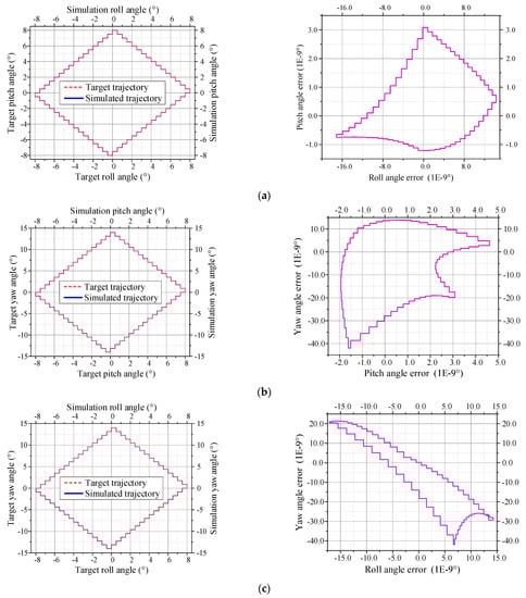

Figure 7.
The simulation trajectories and the corresponding algorithm error on each plane. (a). The quadrilateral trajectory comparison and the algorithm error on the roll-pitch plane, (b). those on the roll-pitch plane, (c). those on the roll-pitch plane, (d). the random trajectory comparison and the algorithm error on the roll-pitch plane.
4.2. Isolation Algorithm Verification
The proposed manipulator capability to stabilize the LOS is tested next. The floor disturbance transmissibility is first compared in the frequency domain. Since the feedforward controller (55) is associated with the manipulator orientation, four pointing directions were considered, whose RPY angles are, respectively, (0°, 0°, 0°), (8.5°, 0°, 0°), (0°, −7°, 0°), and (0°, 0°, 14°). The low-pass filters are both 9-order Chebyshev type II filters whose stop frequencies are 1000 Hz. The high-pass filters are both 2-order filters whose corner frequencies are 10−4 Hz.
As shown in Figure 8, when the feedforward controllers are acted, the maximum attenuation exceeds 50dB in all four cases. Since the phase and gain mismatch, the attenuation effect would degenerate in the transition frequency band of high-pass and low-pass filter, and floor disturbance in the band of 100–700 Hz would be amplified by an active feedforward system, but the amplifications do not exceed 9 dB. The theoretical results derived from Formula (38) are also shown in the figures. It is seen that the theoretical results are well consistent with the passive transmissibility of the virtual system in the low-frequency band. Thus the validation of Formula (38) could be accepted.

Figure 8.
Floor disturbance transmissibility of the pointing and stabilizing manipulator. (a). comparison in the orientation of (0°, 0°, 0°), (b). in the orientation of (8.5°, 0°, 0°), (c). in the orientation of (0°, −7°, 0°), (d). in the orientation of (0°, 0°, 14°).
Furthermore, the vibration isolation effect is compared in the time domain. Disturbance force generated by 0.1–1000 Hz white noise is acted on the support module. The platform orientation jitter is shown in Table 2. It is seen that the jitter levels of all the channels in all four cases sharply go down, the magnitude of platform angular displacement falls to 10−7 rad from 10−5 rad, and the root-mean-square (RMS) level of platform angular displacement reduces by over 95%. The jitter trajectories of the image point and their convex hull are shown in Figure 9. It is seen that the scattered areas in all four cases sharply go down, too. Additionally, the scattered radius standard deviation falls to 10−7 meters from 10−5 meters, which could meet the pointing stability requirements of common optical payloads. Combining the frequency-domain and time-domain results, it could be accepted that the feedforward controller (55) could effectively improve the pointing stability.
Table 2.
RMS level of platform angular displacement of each channel.
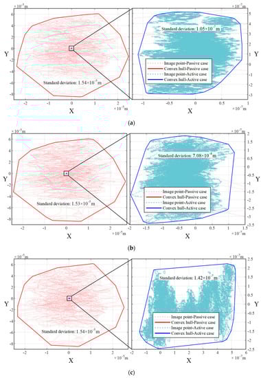
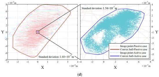
Figure 9.
LOS jitter comparison between the passive isolation and active feedforward isolation. (a). comparison in the orientation of (0°, 0°, 0°), (b). in the orientation of (8.5°, 0°, 0°), (c). in the orientation of (0°, −7°, 0°), (d). that in the orientation of (0°, 0°, 14°).
The stability of IPFL consisting of a feedforward controller (55) and the virtual prototype is tested last. The stability is shown by the bode diagrams of the open-loop transfer function matrices (OLTFM). For convenience, only the elements in the first row and first column of OLTFM and the case of (0°, 0°, 0°) are shown. Besides the Original Support Module (OSM), the manipulator is also installed on a Lighter Support Module (LSM) weighted 9.33 × 10² kg to simulate the case of a larger ratio of the payload mass to the support module mass. A delay of 0.02 s is introduced into all the IPFLs to increase uncertainty.
As shown in Figure 10, the amplitude–frequency curve (AFC) corresponding to OSM is totally below the 0 dB line, i.e., the clockwise encirclement number of the Nyquist plot about the −1 point is zero. Furthermore, considering that the and is inherently stable, i.e., the unstable pole number of the OLTFM is also zero, the IPFL is bound to be stable according to Nyquist stability criterion. Since the smaller support module mass and the AFC corresponding to LSM is above that of OSM and cross over the 0 dB line at the frequency of 5.16 Hz and 5.57 Hz. Then it is seen that the phase-frequency curve corresponding to LSM crosses over the −180° line from above once at 5.42 Hz, and the phase margin is −26.2°. So, the encirclement number is no longer zero; thus, the IPFL corresponding to LSM is unstable. On this basis, the electromagnetic damping of each fine actuator is increased to 1160 N·s/m from 23.2 N·s/m to simulate the larger mode damping ratio case of OSM and LSM. For convenience, they are abbreviated as LDOSM and LDLSM, respectively, here. The passive transmissibility comparison is shown in Figure 11. It is seen that the case of LSM and OSM have similar passive transmissibility, and so do LDOSM and LDLSM, which is consistent with the theoretical result that the transmissibility frees from the support modules. As for stability, as shown in Figure 10, the AFC corresponding to LDLSM comes back below the 0 dB line due to the passive transmissibility attenuation at about 5 Hz, so the encirclement number is zero again, and thus, the IPFL is stable. Combining the stability conditions of OSM, LSM, and LDLSM, it could be accepted that the larger mode damping ratios of or the smaller ratio of the payload mass to the support module mass, the better robust stability of the IPFL.

Figure 10.
Open loop transfer functions of the given channel in four cases.

Figure 11.
Passive transmissibility given in four cases.
5. Conclusions
This paper proposed a novel pointing and stabilizing manipulator that integrated both coarse and fine actuators in parallel. The manipulator is designed to provide small optical space payloads on large spacecraft with independent and large-scale pointing adjustment as well as pointing stabilization at the same time.
A theoretical analysis of the manipulator characteristics was first conducted. Singularity analysis showed that the division of pointing labor is feasible with parallel coarse and fine actuators. Through dynamic analysis, the feed-through characteristic of disturbance transmissibility and the ‘mobile-base’ effect on active control was revealed. The paper further presented a specific operation scheme of the novel manipulator including a large-scale adjustment algorithm and an active vibration isolation algorithm. According to the simulation, using the proposed adjustment algorithm, the prototype could arbitrarily adjust the roll-pitch-yaw angles of the payload pointing within the range of ±8.5° and error below 2 × 10⁻⁸ degrees, and using the proposed active vibration isolation algorithm, the prototype could reduce the pointing direction jitter by over 95%, which reached the level of from the original level of . Therefore, it could be accepted that the parallel integrated scheme of coarse actuators and fine actuators is feasible. The simulation also confirmed some key conclusions of theoretical analysis.
The proposed parallel integrated scheme suits the pointing requirements of future small optical payloads on large spacecraft. The active feedforward method could also be extended to other vibration isolation manipulators. Next, we intend to build an experimental system to validate the solution in practice and achieve the given performance requirements.
Author Contributions
Conceptualization, Z.X.; Methodology, H.Z.; Software, H.Z.; Validation, H.Z.; Investigation, H.Z.; Resources, A.X. and E.Z.; Data curation, A.X. and E.Z.; Writing–original draft, H.Z.; Writing–review & editing, Z.X., A.X. and E.Z.; Project administration, Z.X.; Funding acquisition, Z.X. All authors have read and agreed to the published version of the manuscript.
Funding
This research was funded by National Natural Science Foundation of China grant number 11972343.
Data Availability Statement
No new data were created or analyzed in this study. Data sharing is not applicable to this article.
Conflicts of Interest
The authors declare no conflict of interest.
Appendix A
This section introduced the method to express the kinetic energy of the manipulator’s legs with and . To improve model accuracy while retaining model simplicity, the tiny movable parts such as joint balls would be neglected. As shown in Figure 3, each fine leg is divided into upper and lower parts and linked by a prism joint, and the prism joint in each coarse leg keeps locked. Therefore, the kinematic energy of branch chains includes
kinematic energy of the upper parts fine leg,
kinematic energy of the lower parts fine leg,
kinematic energy of coarse leg,
where , , respectively, represent the centroid velocity of each part. and respectively, represent the angular velocity of fine leg and that of the coarse leg. The definition of each inertial parameter and joint-point velocity can be found in Figure 3.
Linear velocities , and could be represented by and :
The transformation matrices , and are matrices with similar forms. Taking as an example, it has the form of
where is the antisymmetric matrix corresponding to the vector .
According to the structure of the universal joint shown in Figure A1, considering that each leg is linked by the universal joint, the angular velocity of each leg must fulfill
The definition of and can be found in Figure A1. The formula could be equivalently rewritten as
As shown in Figure A1, it could be approximately deemed that each rod is perpendicular to two pivots of the universal joint. So there is the approximation
In addition, the velocity of each joint point fulfills that
The equivalent form is
Combine Equations (A7), (A8), and (A10), and the angular velocity could be approximately expressed as
So far, all the transformations have been obtained. On this basis, the expressions of kinetic energy can be further simplified using the structural characteristics. Assuming that the mass distribution of each leg is approximately axisymmetric, the eccentricity vector of each part can be approximated as
Under the same assumption, the form of inertia tensors can also be simplified. Taking one of the coarse legs as an example, the inertia tensor at the centroid can be generally expressed as
where and are, respectively, the unit vectors of arbitrary two radial directions, and and represent the principal components in the radial and axial directions, respectively. Then according to Formula (A11), the item fulfills
Therefore, the inertia tensors could be approximated as
Combining Formulas (A1)–(A5), (A11), (A12), and (A15), the kinetic energy of all legs could be rephrased as
where
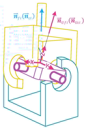
Figure A1.
Schematic diagram of a universal joint.
References
- Jono, T.; Toyoda, M.; Nakagawa, K.; Yamamoto, A.; Shiratama, K.; Kurii, T.; Koyama, Y. Acquisition, tracking, and pointing systems of OICETS for free space laser communications. In Acquisition, Tracking, and Pointing XIII; International Society for Optics and Photonics: Bellingham, WA, USA, 1999; Volume 3692, pp. 41–50. [Google Scholar]
- Kennedy, P.J.; Kennedy, R.L. Direct versus indirect line of sight (LOS) stabilization. IEEE Trans. Control Syst. Technol. 2003, 11, 3–15. [Google Scholar]
- Burnside, J.W.; Conrad, S.D.; Pillsbury, A.D.; Devoe, C.E. Design of an inertially stabilized telescope for the LLCD. In Free-Space Laser Communication Technologies XXIII; SPIE: Bellingham, WA, USA, 2011. [Google Scholar]
- Bernabe, L.; Raynal, N.; Michel, Y. 3POD-A High Performance Parallel Antenna Pointing Mechanism. In Proceedings of the 15th European Space Mechanisms & Tribology Symposium, Noordwijk, The Netherlands, 25–27 September 2013. [Google Scholar]
- Zhang, Y.; Han, H.; Zhang, H.; Xu, Z.; Xiong, Y.; Han, K.; Li, Y. Acceleration analysis of 6-RR-RP-RR parallel manipulator with offset hinges by means of a hybrid method. Mech. Mach. Theory 2022, 169, 104661. [Google Scholar]
- Han, H.; Zhang, Y.; Zhang, H.; Han, C.; Li, A.; Xu, Z. Kinematic Analysis and Performance Test of a 6-DOF Parallel Platform with Dense Ball Shafting as a Revolute Joint. Appl. Sci. 2021, 11, 6268. [Google Scholar] [CrossRef]
- Sun, J.; Shao, L.; Fu, L.; Han, X.; Li, S. Kinematic analysis and optimal design of a novel parallel pointing mechanism. Aerosp. Sci. Technol. 2020, 104, 105931. [Google Scholar]
- Song, Y.; Qi, Y.; Dong, G.; Sun, T. Type synthesis of 2-DoF rotational parallel mechanisms actuating the inter-satellite link antenna. Chin. J. Aeronaut. 2016, 29, 1795–1805. [Google Scholar]
- Sun, T.; Song, Y.; Dong, G.; Lian, B.; Liu, J. Optimal design of a parallel mechanism with three rotational degrees of freedom. Robot. Comput.-Integr. Manuf. 2012, 28, 500–508. [Google Scholar]
- Sun, T.; Zhai, Y.; Song, Y.; Zhang, J. Kinematic calibration of a 3-DoF rotational parallel manipulator using laser tracker. Robot. Comput.-Integr. Manuf. 2016, 41, 78–91. [Google Scholar]
- Kong, Y.; Huang, H. Performance enhancement of disturbance-free payload with a novel design of architecture and control. Acta Astronaut. 2019, 159, 238–249. [Google Scholar] [CrossRef]
- Wu, Y.; Yu, K.; Jiao, J.; Cao, D.; Chi, W.; Tang, J. Dynamic isotropy design and analysis of a six-DOF active micro-vibration isolation manipulator on satellites. Robot. Comput.-Integr. Manuf. 2018, 49, 408–425. [Google Scholar] [CrossRef]
- Beijen, M.A.; Heertjes, M.F.; Van Dijk, J.; Hakvoort, W.B.J. Self-tuning MIMO disturbance feedforward control for active hard-mounted vibration isolators. Control Eng. Pract. 2018, 72, 90–103. [Google Scholar]
- Qian, Y.; Xie, Y.; Jia, J.; Zhang, L. Development of Active Microvibration Isolation System for Precision Space Payload. Appl. Sci. 2022, 12, 4548. [Google Scholar]
- Doré Landau, I.; Alma, M.; Constantinescu, A.; Martinez, J.J.; Noë, M. Adaptive regulation—Rejection of unknown multiple narrow band disturbances (a review on algorithms and applications). Control Eng. Pract. 2011, 19, 1168–1181. [Google Scholar]
- Aranovskiy, S.; Freidovich, L.B. Adaptive compensation of disturbances formed as sums of sinusoidal signals with application to an active vibration control benchmark. Eur. J. Control 2013, 19, 253–265. [Google Scholar]
- Landau, I.D.; Airimitoaie, T.; Alma, M. IIR Youla–Kucera Parameterized Adaptive Feedforward Compensators for Active Vibration Control With Mechanical Coupling. IEEE Trans. Control Syst. Technol. 2013, 21, 765–779. [Google Scholar] [CrossRef]
- Yun, H.; Liu, L.; Li, Q.; Yang, H. Investigation on two-stage vibration suppression and precision pointing for space optical payloads. Aerosp. Sci. Technol. 2020, 96, 105543. [Google Scholar] [CrossRef]
- Yang, X.; Wu, H.; Li, Y.; Kang, S.; Chen, B.; Lu, H.; Lee, C.K.M.; Ji, P. Dynamics and Isotropic Control of Parallel Mechanisms for Vibration Isolation. IEEE/ASME Trans. Mechatron. 2020, 25, 2027–2034. [Google Scholar]
- Yang, X.; Wu, H.; Chen, B.; Kang, S.; Cheng, S. Dynamic modeling and decoupled control of a flexible Stewart platform for vibration isolation. J. Sound Vibr. 2019, 439, 398–412. [Google Scholar]
- Yi, S.; Yang, B.; Meng, G. Microvibration isolation by adaptive feedforward control with asymmetric hysteresis compensation. Mech. Syst. Signal Proc. 2019, 114, 644–657. [Google Scholar] [CrossRef]
- Wu, L.; Huang, Y.; Li, D. Tilt Active Vibration Isolation Using Vertical Pendulum and Piezoelectric Transducer with Parallel Controller. Appl. Sci. 2021, 11, 4526. [Google Scholar]
- Li, F.; Yuan, S.; Qian, F.; Wu, Z.; Pu, H.; Wang, M.; Ding, J.; Sun, Y. Adaptive Deterministic Vibration Control of a Piezo-Actuated Active–Passive Isolation Structure. Appl. Sci. 2021, 11, 3338. [Google Scholar]
- Sun, X.; Yang, B.; Gao, Y.; Yang, Y. Integrated design, fabrication, and experimental study of a parallel micro-nano positioning-vibration isolation stage. Robot. Comput.-Integr. Manuf. 2020, 66, 101988. [Google Scholar] [CrossRef]
- Kong, Y.; Huang, H. Vibration isolation and dual-stage actuation pointing system for space precision payloads. Acta Astronaut. 2018, 143, 183–192. [Google Scholar]
- Hindle, T.; Davis, T.; Fischer, J. Isolation, Pointing, and Suppression (IPS) System for High-Performance Spacecraft; SPIE: Bellingham, WA, USA, 2007. [Google Scholar]
- Tang, L.; Zhang, K.; Guan, X.; Hao, R.; Wang, Y. Dynamic modeling and multi-stage integrated control method of ultra-quiet spacecraft. Adv. Space Res. 2020, 65, 271–284. [Google Scholar] [CrossRef]
- Friederike, G.; Andreas, R.; Holger, J.; Ulrich, L.; Enrico, P.; Manuel, W.; Jürgen, W.; Stefanos, F. Pointing and Control System Performance and Improvement Strategies for the SOFIA Airborne Telescope; SPIE: Bellingham, WA, USA, 2016. [Google Scholar]
- Paul, J.K.; Edward, D.; Ulrich, L.; Enrico, P.; Stefan, T.; Hans-Peter, R.; Manuel, W.; Jürgen, W. Active Damping of the SOFIA Telescope Assembly; SPIE: Bellingham, WA, USA, 2012. [Google Scholar]
- Paul, K.; Rick, B.; Jorge, G.; Ulrich, L.; Hans, K.; Stefan, T.; Jörg, W. SOFIA Telescope Modal Survey Test and Test-Model Correlation; SPIE: Bellingham, WA, USA, 2010. [Google Scholar]
- Sacks, L.W.; Blaurock, C.; Dewell, L.D.; Tajdaran, K.; Liu, K.; Collins, C.; West, G.J.; Ha, K.Q.; Bolcar, M.R.; Crooke, J.A.; et al. Preliminary Jitter Stability Results for the Large UV/Optical/Infrared (LUVOIR) Surveyor Concept Using a Non-Contact Vibration Isolation and Precision Pointing System; SPIE: Bellingham, WA, USA, 2018; Volume 10698. [Google Scholar]
- Larry, D.D.; Kiarash, T.; Raymond, M.B.; Kuo-Chia, L.; Matthew, R.B.; Lia, W.S.; Julie, A.C.; Carl, B. Dynamic Stability with the Disturbance-Free Payload Architecture as Applied to the Large UV/Optical/Infrared (LUVOIR) Mission; SPIE: Bellingham, WA, USA, 2017. [Google Scholar]
Disclaimer/Publisher’s Note: The statements, opinions and data contained in all publications are solely those of the individual author(s) and contributor(s) and not of MDPI and/or the editor(s). MDPI and/or the editor(s) disclaim responsibility for any injury to people or property resulting from any ideas, methods, instructions or products referred to in the content. |
© 2023 by the authors. Licensee MDPI, Basel, Switzerland. This article is an open access article distributed under the terms and conditions of the Creative Commons Attribution (CC BY) license (https://creativecommons.org/licenses/by/4.0/).