Time Evolution of the Modulus of Elasticity of Metakaolin-Based Geopolymer

Abstract

The objective of the research is to develop a new family of geopolymeric materials and to use an experimental methodology to characterize the mechanical behavior of the materials obtained by alkaline activation of metakaolin using a compound activator. The researchers also intend to study the unknown time evolution of the modulus of elasticity and the influence of the composition of the aggregates on the strength of the material. Like the material’s strength, the results have a direct influence on structural safety evaluations. For the analysis of the mechanical properties of the mixtures, different types of tests were carried out: Flexural and compression tests on parallelepipeds and compression tests on cylinders were performed to assess the main strength characteristics of metakaolin-based geopolymers. Regarding the aggregate composition, the results show that the correction of the aggregate particle size line did not improve the mechanical properties. From about 400 h of curing, at ambient temperatures, the mechanical properties of the geopolymeric material are almost invariable. The highest value of the elastic modulus of elasticity occurs around 420 h, at about 18 GPa. The modulus of elasticity is independent of test load rate as per standards, and 1.7‰ strain was observed during maximum compressive stresses in the rupture tests. Also, the secant modulus values at 60% and 80% of maximum stress are within 12% of the value at 40% of maximum stress.

1. Introduction

Some geopolymers are materials and products with satisfactory physicochemical, mechanical, and thermal properties for construction in general. Therefore, they have great potential to be a sustainable alternative to Portland cement. Properties such as good adhesion to other materials such as steel, glass, ceramics, fresh concrete and old substrates, high compressive and abrasion resistance, low shrinkage and thermal conductivity, fast and controlled curing, high acid resistance, high pH to protect reinforcement, reduced emission of pollutants, and good fire resistance have shown the good performance of geopolymer materials in construction [1,2,3,4,5].

In this context, the metakaolin-based geopolymer is one of the alternatives. Metakaolin is a kaolinitic clay of high fineness and reactivity. When it is calcined, a process that allows almost complete dehydroxylation of the raw material, it becomes an amorphous and irreversible phase with pozzolanic properties. When this amorphous metakaolin is subjected to the geopolymerization process (alkaline activation), the geopolymer is formed [6].

Geopolymerization consists of an exothermic chemical reaction between an aqueous solution of high alkalinity, called an activator, and materials of geopolymer origin composed of minerals such as silica and alumina, resulting in polymers with polysialate-like bonds. The quality of the geopolymer depends essentially on the type of starting material [7].

Several works on geopolymerization have been developed in the laboratory of DEC-FCTUC. Some are related to structural applications [8], others to the development of geopolymerized material [9]. Other work has been related to the evaluation of the resistance of geopolymers [10,11,12,13] and the modulus of elasticity of concrete in different situations [14,15].

For example, Oliveira [10] demonstrated that the mechanical properties of metakaolin-based geopolymers remained practically constant from the 14th day of maturity of the samples. It was also found that the activator was more effective between a ratio of 1:1.75 and 1:2 (hydroxide:silicate), and achieved better resistance, although the maximum value of the elastic modulus was just outside this range.

Fernandes [11] analyzed the effect of curing temperature of geopolymer blends composed of two types of metakaolin: white “MetaMAX^®® HRM” and brown “ARGECO”. He concluded that curing temperatures above 30 °C led to a loss of the resistant properties.

Guerra [12], analyzing the influence of the percentage of metakaolin in the mixture and also the change in the composition of aggregates with granulometric variations, to evaluate their effects on tensile and compressive strength, concluded that the amount of binder is not a fundamental parameter to improve the resistance of geopolymers. In turn, changing the composition of the aggregates in the mixes did not provide conclusive results.

The authors have already performed some tests on geopolymer-reinforced beams [8] and they found that it would be very important to study the basic mechanical characteristics of the material, such as, the shrinkage in fly ash-based geopolymers. Regarding the modulus of elasticity of metakaolin-based geopolymers, the authors did not find any work that indicates the time evolution of this parameter. Knowledge of this mechanical characteristic of the material is fundamental, not only for structural analysis. Working in the context of the finite element method and also verifying the safety conditions of structures in relation to deformation can be mentioned as examples of this. This article presents some of the findings that would be very useful for the structural design of structural members. The way in which the strength rises over time and the necessary curing time are also 2 important features to analyze.

In this regard, the following must be said. In the bibliography it is possible to find several works on the mechanical characteristics of concrete, including the modulus of elasticity. Recently, these works have focused on material that has been altered, say, either by partially replacing the binder, or by adding other aggregates (for example, recycled aggregates or other industrial waste), or by adding fibers, or by using nanoparticles, etc.

The number of bibliographical references of works that only include geopolymers is relatively small. In fact, the overwhelming majority addresses slag/fly ash-based geopolymers. Even though they address the modulus of elasticity, this value is rarely identified in more than a given age (14 days or 28 days); exception for Waqas et al. [16], who evaluated the modulus of elasticity at 24 h, 3 d, 7 d, 14 d, 28 d, 56 d, and 90 d. In this regard, it is worth quoting the review by Mohammed A. [17]. In this review, the issue of the relationship between the modulus of elasticity and the compressive strength of the geopolymer is addressed. All 4 works cited have used fly ash as a binder.

Works that address the modulus of elasticity and include metakolin in the composition of the geopolymer are very rare. Amin et al. [18], using a metakaolin-based (63% SiO₂; 31% Al₂O₃) geopolymer, cured at 80 °C for 24 h, have determined the highest value of modulus of elasticity (35.6 GPa at 28 days) ever found. Rocha et al. [19] have obtained a much lower value (~7 GPa at 28 days); metakaolin (48% SiO₂; 45% Al₂O₃). Either Ahmed et al. [20], or Alsaif et al. [21] determined values similar to those found in this work. However, not a single study was found that would present the time evolution of this parameter.

Another factor considered in this work concerns the practical applicability of the material. For the authors, it is interesting to address materials whose availability is likely to be already applied in civil construction. But doubts remain regarding the variability of results, which makes the adoption of this material in construction unfeasible, for the time being.

2. Experimental Procedure

2.1. Materials

Metakaolin (brick paint) was supplied by the French company Argeco Développement. According to the company, it was subjected to a dehydroxylation reaction at a temperature of 750 °C and the metakaolin particles have a diameter of less than 90 µm [22].

The sand used is natural sand from the Coimbra region with a density of about 1650 kg/m³ and a specific gravity of about 2600 kg/m³. The sieve analysis of the sand is shown in

Table 1. Sieve analysis: Percent passing.

Sieve (mm)	Sand	Gravel	Filer	MN
4.750	100.0	100.0	100.0	100.0
2.000	94.0	0.0	100.0	52.5
0.850	67.7	0.0	100.0	41.4
0.425	33.9	0.0	100.0	27.2
0.250	14.4	0.0	100.0	19.1
0.150	4.5	0.0	100.0	14.9
0.075	0.8	0.0	90.0	12.0
0.050	0.0	0.0	0.0	0.0
Deposit	-	-	-	-
	42%	45%	13%	100%

. The grain size distribution line is shown in Figure 1.

The gravel (from the company Betão Liz [23]; GPS: 40.255788, −8.444268) was supplied in the form of tout-venant. For the present work, limestone gravel was chosen, sieved through a 4.75 mm sieve and retained on a 2 mm-diameter sieve (Table 1 and Figure 1). The standard EN 196-1 [24] recommends this dimension for the maximum allowable diameter of aggregates in relation to the construction of prismatic specimens built for this work: 160 mm × 40 mm × 40 mm.

An alkaline activator was used to activate the binder (metakaolin), which consisted of sodium hydroxide (NaOH) and sodium silicate (Na₂SiO₃) in a 1:2 ratio. To produce sodium hydroxide solutions (10 M), pellets with 98 % to 99 % purity were dissolved in tap water until the target concentration was reached; 1 weight of sodium hydroxide with 2.5 weight of water. Sodium silicate was purchased from the company “Sociedade Portuense de Drogas, S.A.” [25], under the name sodium silicate D40. Its chemical composition is indicated in

Table 2. Chemical composition of the sodium silicate solution.

SiO2 (wt.%)	Na2O (wt.%)	Al2O3 (wt.%)	H2O (wt.%)
27.3–28.3	8.2–8.6	<4.0	59.1–64.5

.

The fineness modulus of the filler is 0.063 µ, the moisture content is 0% and the specific gravity is 2810 kg/m³. It was provided by the production company Comital [26].

2.2. Mixtures

Three different mixtures were performed to prove certain resistant properties of geopolymers. The first one, defined by MW (

Table 3. Mix portions.

Mix	MW	MC	MN
	1:2.5:0.86	1:2.5:0.75	1:2.5:0.79
Metakaolin	750 g	809 g	808 g
Sand	1875 g	1314 g	849 g
Filer	--	--	263 g
Gravel 2 mm	--	708 g	910 g
NaOH	215 g	203 g	213 g
(Na2SiO3)	430 g	407 g	426 g

), was previously used by Lopes et al. [8] and Oliveira [10]. The indicated quantities allow the production of 6 parallelepiped specimens of 160 mm × 40 mm × 40 mm. The mix proportion (aggregate:binder:activator) is shown in Table 3 (2nd line). The second mixture, MC, was developed by Freitas [13]. This mixture contains limestone crushed through a 4.75 mm sieve and retained on a 2 mm sieve. The constituent of the mixture is listed in Table 3.

Finally, a new mixture was created that improved the granulometric line of the previous mixtures. As is known from the study of concrete, granulometry determines the compactness of concrete and thus its physical and resistance properties. The higher the compactness of granulometric compositions, the lower the volume of voids between particles and the greater the possibility of reducing the volume of the mixture. Higher compactness favors obtaining a more resistant concrete with low porosity, low shrinkage, and high durability [27]. The most compact granulations are obtained with a high percentage of coarse aggregates, and in this sense the mixing requires lower quantities of binder, while on the other hand, the maximum dimension of the aggregates is limited by the free dimensions of the pieces to be concreted. On the contrary, a less compact granulometry leads to concrete with low workability, which crumbles easily. In this sense, it is necessary to adapt the mix to an optimal content of fine aggregates [27].

So, the last objective of this new mixture was to improve the resistance of the mixtures. In fact, the granulometric line of the MC mixture has deficiencies in terms of the percentage of finer particles. This deficiency is aggravated in the MW mixture. Therefore, in this blend, part of the sand and gravel was replaced by fillers. The constituents of the new blend are listed in Table 3.

2.3. MN Mix Design

The optimal amounts in the MN mixture were estimated by adjusting the granulometry of the aggregates that make up the mixture. The percentage of each component was determined to approximate (Figure 1) such a combination to the reference line (Faury), normally used in the production of concrete. Table 1 shows the past percentages of the aggregates that make up the MN mix. The optimum composition of the mix was made with 42% sand, 45% gravel, and 13% filler.

In constructing, the reference line, a dimension of 0.050 mm was considered for the origin of the abscissa, which corresponds to the minimum size of the filler. The linear or Pearson correlation coefficient (r) between the Faury and MN line was estimated to be 0.995; 0.896 to MC line. Figure 1 shows the granulometric lines of the aggregate used in the composition of the MN mixture, the Faury line, and grain size distribution line of the MW, MC, and MN mixtures.

2.4. Mixtures and Parallelepiped Samples

The mixtures were performed at room temperature (~21 °C) using an electric mixer. First, the metakaolin (dry) was mixed with the sand and the filler. Then the activator was gradually added. Finally, the gravel was added, with the mixer always switched on. The process takes about 5 min.

After the mixture was poured into the 2 molds (6 parallelepiped specimens; 40 mm × 40 mm × 160 mm), it was vibrated for about 1 min to ensure maximum compaction of the mixture. The bottoms of the molds were protected with plastic sheets, and later on, the top, to avoid the evaporation of the liquid phase of the mixture (Figure 2).

Curing was carried out in laboratory ambient (T = 20 ± 2 °C). The demolding was carried out according to standard EN 196-1 [24], usually within a period of 24 h. Before the tests, the mass of each sample and the measurements (using a caliper) of the width b and the height h of the cross section were recorded.

2.5. Cylindrical Specimens

Specimens must be either shaped (cylinders or prisms) or core drilled and must meet the requirements of EN 12390-1 [28] or EN 12504-1 [29]. In the case of cylinders, the diameter d shall be at least 3.5 × Dmax, where Dmax is the maximum dimension of the aggregate. The ratio between the length L of the specimen and the dimension d must satisfy the condition 2 ≤ L ≤ 4.

The mold used to construct the cylindrical specimens consisted of an ordinary 350 mm long PVC (Polyvinyl chloride) pipe with an approximate inner diameter of 107 mm, as shown in Figure 2. These values comply with standard EN 12390-1 [28]. Before the tests, the geometric characteristics were recorded.

Each cylindrical sample was instrumented with 3 FLK-6-11 strain gauges with a resistance of 120 Ω and a gauge factor of 2.12, manufactured by Tokyo Sokki Kenkyuio Co., Ltd., (Tokyo, Japan) (Figure 3). The placement of the strain gauges considered 3 details: (i) they were bonded halfway up the sample; (ii) the strain gauges were bonded so that the strains were measured parallel to the longitudinal axis of the sample; and (iii) they were evenly spaced along the circumference of the sample. This arrangement allows the average length of the sample subjected to axial compressive stress to be accurately measured, even when some eccentricity of action is present.

2.6. Experimental Methodologies

The tests performed to determine the mechanical strength of the specimens and the modulus of elasticity were carried out in accordance with applicable standards: EN 196-1 [24], EN 12390-13 [30], EN 12390-3 [31], and EN 12390-5 [32].

The flexural strength test was the first to be performed on parallelepiped specimens according to EN 12390-3 [27]. The two resulting “halves” constitute the compression test specimens. A Servosis ME -402 series electromechanical compression machine and one load cell (CLC—200 kN) were used for this purpose. The equipment was completed with a data logger (TSD-602; to record the load and strains) and two 8 mm neoprene sheets. The tests were performed with a deformation control planned in two different phases: first, the action was applied at a rate of 0.1 mm/s up to a load of about 0.3 kN; then, at a rate of 0.004 mm/s, up to failure. The test lasted for about 3 min. In the compression test, the action was first applied at a rate of 0.1 mm/s up to a load of about 3 kN; then the rate was reduced to 0.013 mm/s, up to failure. The test lasted for about 3 min. Suitable equipment was also used in this compression test, with two square compression plates of 40 mm on each side. The generation of the cones was checked; a requirement specified in standard EN 12390-3 [27].

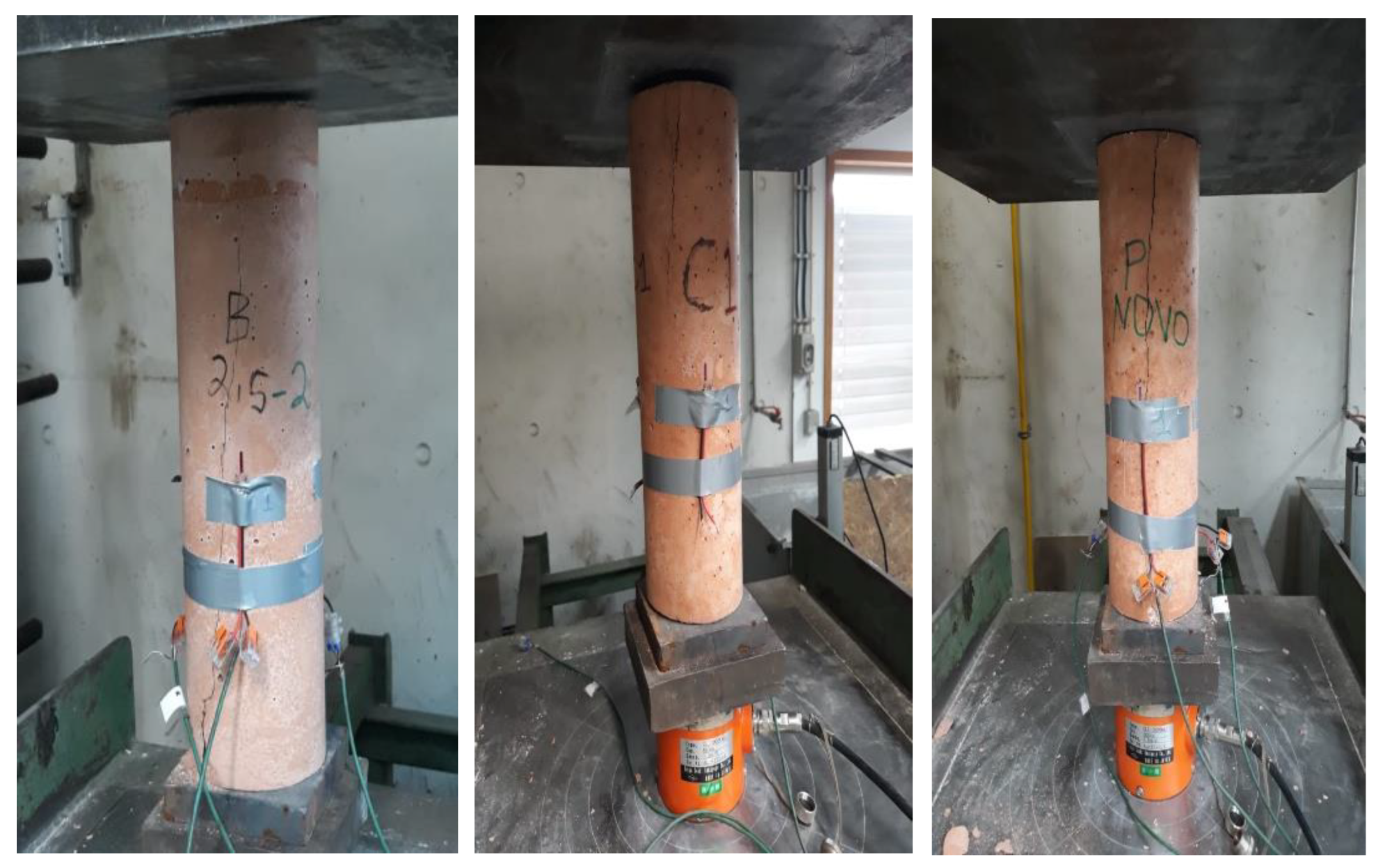
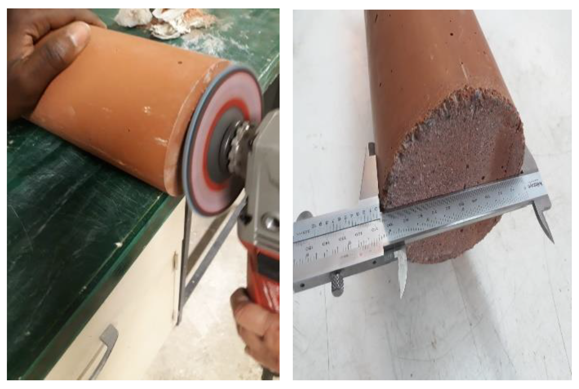
The tests to determine the modulus of elasticity were performed on the cylindrical specimens. The methodology used is based on an adaptation of method B, which is described in standard EN 12390-13 [30]. Before the actual test, the top and bottom surfaces of the specimens had to be straightened: They should be flat and perpendicular to the axis of the sample (Figure 4). This is to ensure an even distribution of stresses on the surfaces of the sample. In this context, it is important to mention five other strategies that were used to perform the test:

• Use of specimens long enough to relieve possible stress concentrations;
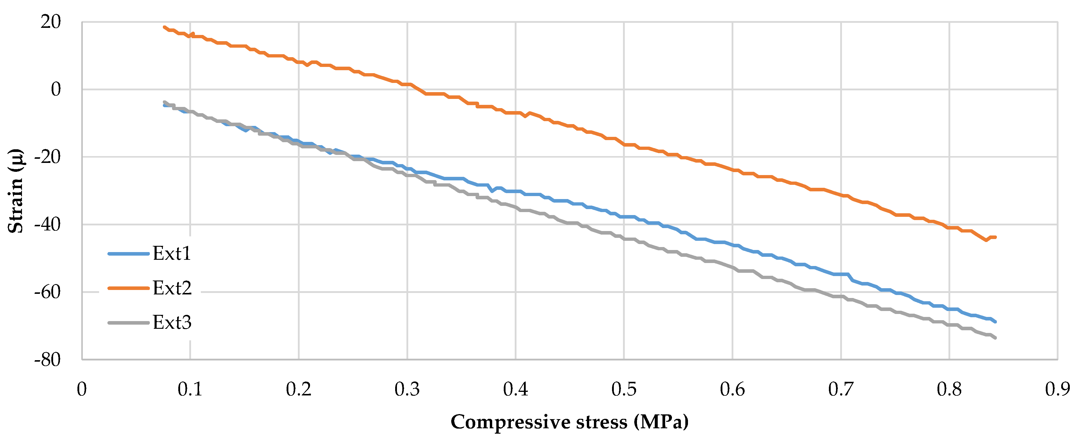
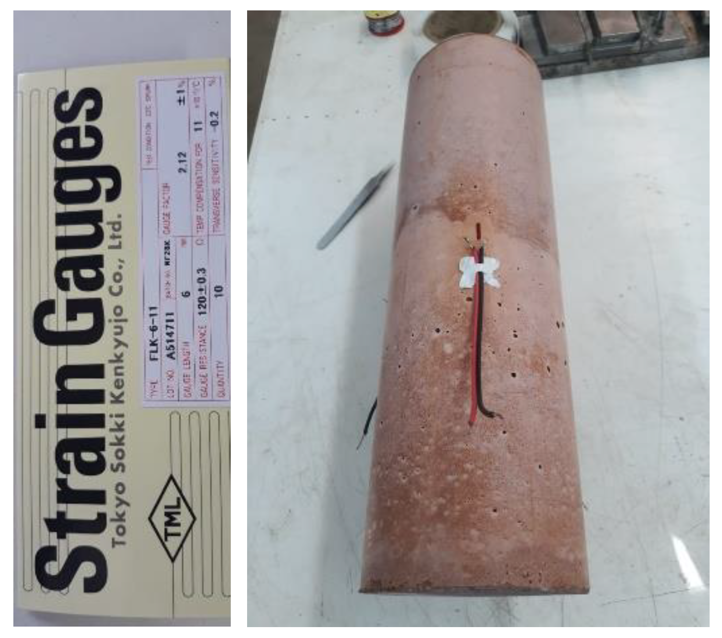
• Use of three strain gauges that guarantee the reliability of the average strain values;
• Use of neoprene rubbers to eliminate possible surface irregularities;
• The hinge that can partially eliminate possible deviations of these surfaces from the normal to the axis of the specimen; and
• When placing the specimen, care was taken to place it centrally to ensure an even distribution of the load on the specimen.

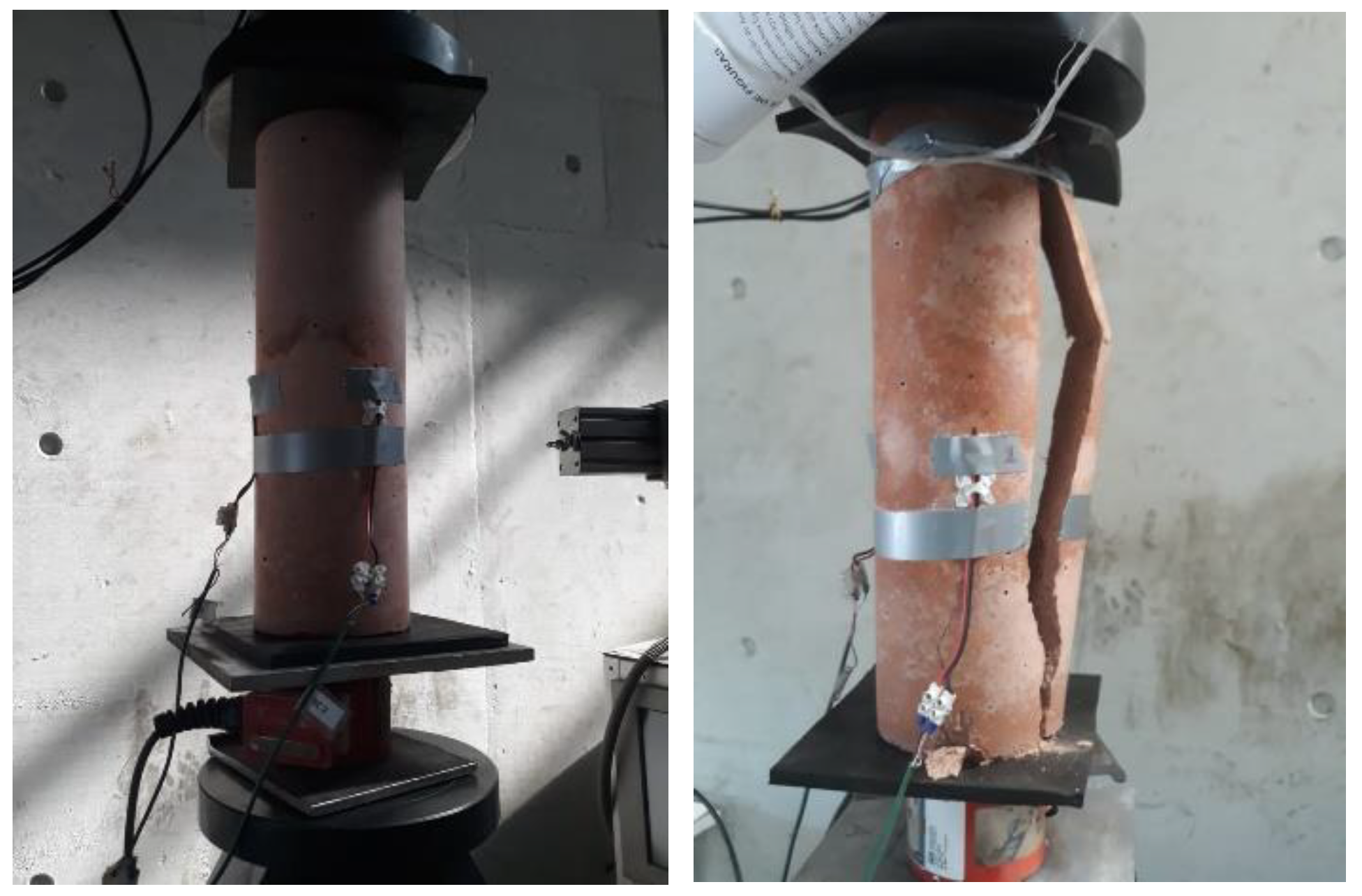
The “setup” of the test began by placing a washer and a metal plate on the bottom plate of the compression machine (Figure 5). The washer forms a partial hinge that, along with the hinge on the top plate of the Servosis electromechanical press, helps to center the action. Then, the load cell (for measuring the axial force) and another metal plate is placed. The specimen was finally placed between this last metal plate and the upper plate of the press, together with the neoprene sheets (8 mm), one on each side.

The most important result of the tests to be performed was to determine the time evolution of the elastic modulus. But in this series of tests there were several alternative objectives. From the beginning, it was important to ensure that each test would take place in an elastic regime to ensure the integrity of the sample for the next test. It was also interesting to understand the extent to which it would be possible to guarantee this integrity, i.e., at what stress level would the behavior plastic degrade the sample. It was also interesting to see if the test load ratio would in any way affect the value of the modulus of elasticity. Considering these and many other issues, it was determined that the test methodology used in this work deviated from the above standard.

Another point that can already be highlighted as complementary to the provisions of method B in, standard EN 12390-13 [30], concerns the load ratio chosen for the tests. As an alternative to the use of increasing stress, as recommended in the standard, the tests were performed with deformation control. Obviously, there is a dependence between the strain rate and the applied stress rate. In any case, much lower load ratios than those recommended in the standard were chosen from the outset to ensure the integrity of the sample.

Also, as can be seen in the next section, this methodology was updated during the tests, as some answers were found, and new questions arose.

Regarding the operationalization of the test, it is important to add the following. After centering the specimen in the testing machine, a preload was applied for visual inspection of the strain gauges, as provided for in the standard. Similar strain steps on the three strain gauges would guarantee the centering of the specimen. If necessary, the specimen was fully unloaded, and its position corrected. After correcting the positioning, the test was ready to start.

Thus, each test was divided into two parts: In the first part, the preload cycles were performed, and in the second part, the load cycles were performed. The maximum compressive stress should have been limited to fc/3, and maintained for about 60 s. This limit was not always met. At this time, fc would represent the expected value for the maximum compressive stress of the sample. During unload, a similar deformation rate was selected down to a residual stress, of the order of 0.5 MPa, to avoid decentralization of the sample. After unloading, an interval of about 30 s would be expected.

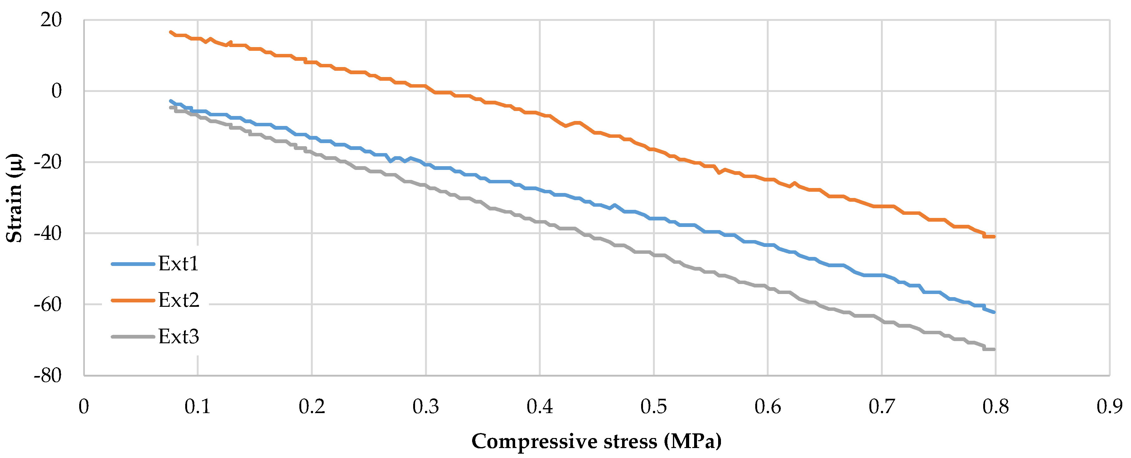
As mentioned above, in this work a slightly different methodology was used than the one given in standard EN 12390-13 [30]. In this standard, the test allows the evaluation of the maximum value of the modulus of elasticity in a single time, that is, a single test on the sample with 28 days of maturity. In this work, the methodology consisted in assessing the time evolution of the modulus of elasticity through tests performed punctually on different days of curing of the sample. Thus, the average value of the modulus of elasticity under compression, on a given curing day, is obtained from the average values obtained from the loading cycles considered. In turn, the average value E_m in each loading cycle is determined by the average change in stress Δσ, with respect to change in strain Δε, i.e.,

$${\mathrm{E}}_{\mathrm{m}}={\left(\frac{\Delta \mathrm{\sigma }}{\Delta \mathrm{ϵ}}\right)}_{\mathrm{m}\mathrm{e}\mathrm{d}}$$

(1)

It is important to emphasize again that, although this work is based on an extensive set of standards, the methods used in the tests have been successively adapted to meet not only the main objective of the work, but also other issues raised, namely the influence of the strain rate imposed on each loading cycle.

3. Test Results

3.1. Flexural and Compressive Strengths

The MW mixture was studied first, and the MN mixture was studied last.

Table 4. Flexural strength.

Mix	Freitas (1)	Freitas (2)	MW	Freitas (3)	MC	MN
σt	4.80 MPa	4.50 MPa	4.54 MPa	4.68 MPa	4.59 MPa	4.72 MPa
STDEV	--	--	0.12 MPa	--	0.47 MPa	0.28 MPa
CV	--	--	2.6%	--	10.2%	6.0%

shows the average values of the flexural strength σ_t, the corresponding standard deviations STDEV, and coefficients of variation CV. Figure 6 shows the mean values and confidence interval (95%) for each mix. This figure also shows the average values obtained by Freitas [13]: 2 values for a mixture similar to MW; the other for a MC-like mixture.

As for the quality of the tested specimens, the MC mixture is the worst. Actually, the coefficient of variation should be less than 10%. As for the global average values, the results are reasonably homogeneous, regardless of the aggregate composition: σ_t,min = 4.50 MPa; σ_t,max = 4.80 MPa. Considering the results obtained now, it can be said that the improvement of the compactness of the aggregates contributes little or nothing to the flexural strength of the geopolymer.

Table 5. Compressive strength.

Mix	Freitas (1)	Freitas (2)	MW	Freitas (3)	MC	MN
σc	36.1 MPa	32.3 MPa	35.1 MPa	38.3 MPa	36.3 MPa	35.5 MPa
STDEV	--	--	1.8 MPa	--	2.1 MPa	2.6 MPa
CV	--	--	5.1%	--	5.7%	7.4%

and Figure 7 show the corresponding values of compressive strength σ_c. Considering the values of the coefficient of variation, the quality of the produced specimens is good. It is also confirmed that the compressive strength did not increase with aggregate compaction. The authors cannot explain the fact that these more compact mixtures do not show greater resistance. Perhaps, the filler material is responsible for this conclusion.

3.2. Modulus of Elasticity Test—MW1 Sample

Regarding the MW mixture, the first to be analyzed, 2 cylindrical specimens named MW1 and MW2 were built. For the MW1 sample, the beginning of the tests occurred after 40 h and after 26 h for MW2 sample.

The tests performed with the aim of evaluating the time evolution of the modulus of elasticity were based on a new methodology developed and perfected during the laboratory work. Although standard EN 12390-13 [30] was used as often as possible, as will be seen, this standard could not answer all the questions that arose.

By test, a “battery of tests” is meant. First, in order to determine the development over time, it was necessary to perform the tests on different curing days. Second, each result represents multiple tests, i.e., multiple load/unload cycles. Third, preload cycles and other unreported tests also count. In other words, in addition to the material, curing time, dimensions, loading rate, maximum load, and the test method itself, each sample was subjected to several tests at different curing times. Assuming one test per specimen, one would have to build dozens of cylindrical specimens tested in different sets and with different curing times. This strategy would be difficult to implement.

In this type of test (loading/unloading cycles), care must be taken to center the sample in the compression machine so that the action is concentric. This method consists in reducing the deviations between the values measured with the 3 strain gauges. Appendix A presents an example of placing cylindrical specimens in the apparatus.

Another concern throughout the test battery was to ensure that all loading and unloading cycles took were elastic. If not, any plastification would prevent reuse of the sample. It should be noted that this objective is not a requirement of the aforementioned standard insofar as it is assumed that the sample will break after the 1st test. An example of this confirmation is shown in Appendix B.

In addition to guaranteeing the elastic behavior of the specimen, it was interesting to know to what extent the load ratio would influence, or not, the calculated result of the modulus of elasticity. It is important to keep in mind that standard EN 12390-13 [30] requires that the load ratio be between 400 and 800 kPa/s. Now, given the initial self-imposed limit of 1 MPa, it is immediately checked that this requirement of the standard could not be verified. It is important to remember that the modulus of elasticity results from the slope of the stress-strain trend line, which can be easily obtained from a linear regression. With this aim, the more points there are, the better. In this work, with very few exceptions, a minimum number of 30 points was ensured, which in a recording obtained at a frequency of 1 Hz, is equivalent to a clean recording of 30 s, or about 40 s of testing. In this context, the maximum effective velocity which might initially be imposed on the sample would be limited to 25 kPa/s.

As mentioned above, the tests were carried out under control of deformation. However, this rate of deformation imposed on the press does not fully reflect the effective strain rate confirmed in the sample. Indeed, between the compression machine plates there is all the equipment used for the “setup”, namely the neoprene sheets, which are responsible for a significant part of the absorbed deformation. Assuming an effective velocity on the sample of about 25 kPa/s, as a limit, this corresponds to about 1.25 × 10⁻⁶/s (E~20 GPa), or an effective deformation of the sample of 0.001 mm/s (L = 350 mm). Since neoprene sheets are involved, it quickly became clear that this deformation rate could be 4 times higher to ensure the desired recordings on the sample. It should also be noted that when a cycle was carried out at the same deformation rate as the previous cycle, the effective deformation rate measured on the sample was slightly higher.

Regarding the influence of the load ratio on the measured modulus of elasticity, it can be observed in

Table A3. Deviations and values from load-unload cycles. MW1 sample.

	Δεmax	MDev	Em (GPa)	σ0 (MPa)	∂σ/∂t (kPa/s)
1stLD	6.9%	--	15.06	0.107	88.1
1stUL	--	--	15.23	0.059	−156
2ndLD	6.5%	−1.6%	15.02	0.076	35.3
2ndUL	--	--	15.16	0.025	−70.4
3rdLD	5.3%	2.1%	15.03	0.050	43.6
3rdUL	--	--	15.17	−0.008	−71.0
4thLD	5.1%	1.7%	15.06	0.020	48.7
4thUL	--	--	15.13	−0.012	−72.6
5thLD	4.3%	2.5%	15.11	−0.002	141
5thUL	--	--	15.14	−0.003	−161

(in Appendix B) that between the 4th and 5th load cycle the deviation of the modulus of elasticity is less than 0.4% when the loading rate is almost tripled.

3.2.1. Time Evolution of the Modulus of Elasticity

Figure 8 shows the time evolution of the average values of the modulus of elasticity E as a function of the curing time of the MW1 specimen. The last point (in red; not considered for the trend line) represents the rupture of the sample. In the same figure, the trend line of the results can be seen (assumed 2nd degree polynomial; trend line that best fits the values). Starting from this line, the result at T = 96.6 h is about 10% away.

Once more, several questions were formulated in advance of the tests. First, the initial age of the specimen in the 1st test, due to the time interval until the minimum resistance is reached and the time required to instrument the specimen, i.e., to bond the strain gauges. For this sample, it was possible to start the tests after 40 h. When evaluating the results, other questions arose: what is the best way to describe the evolution of the modulus of elasticity of the material over the time, and when does the positive evolution of this value end? For this sample, it was decided to focus the tests on the initial phase of curing. It was not possible to determine the point in time after which it would no longer be worthwhile to continue the tests.

3.2.2. Rupture of the MW1 Sample

This first sample began the development of a methodology that allowed consistent analysis of key aspects of the time evolution of the modulus of elasticity of alkali-activated metakaolin. However, there have been innumerable undescribed tests on hypotheses raised, which are not interesting to report, since they do not involve any scientific interest for the formulated objective. Figure 9 shows the range of compressive stresses imposed {σ_min–σ_max} on the sample on each day of the experiment, as well as the number n of load cycles performed.

The rupture of the MW1 sample was caused by longitudinal cracking in the 13th test (Figure 5). As can be seen in Figure 8, the last values already show a certain weakness of the sample.

There are some suspicions in connection with the verified rupture. One of the justifications could be the concentration of stresses near part of the boundaries of the compressed surfaces, due to the lack of perpendicularity with respect to the axis of the sample. This hypothesis was not accepted, since all the concerns were taken when straightening these surfaces and, moreover, the neoprene sheets were uniformly compressed. Another alternative was to allow for presumed fatigue of the specimen. In other words, too many tests were performed in such a short period of time, reaching stresses close to 64% of the expected value of the maximum compressive stress. One can only speculate on this issue. For some reason, the standard EN 12390-13 [30] requires that the specimen be brought to rupture after each test. In any case, all these issues have been referred to the testing of the new sample in order to improve the methodology used.

3.3. Modulus of Elasticity Test—MW2 Sample

The now improved methodology was to schedule 3 loading-unloading cycles for all tests, as specified in the standard. In the first days of curing, 2 tests per day were performed to obtain more points on the chart. After that, only one test per day was performed. Since the speed does not affect the results, all loading cycles were performed at the same speed: 12 kPa/s in the 1st test; 24 kPa/s in the last. The maximum stresses reached in each test started at 0.7 MPa and were gradually increased up to 5 MPa (20% of the expected value for rupture of the sample under compression). The parameter σ0 was always kept below 0.1 MPa, except in the last test, where it reached 0.3 MPa.

The average values of the modulus of elasticity E, obtained up to the 16th test, are shown in Figure 10 as a function of the curing time of the sample. The value for the 1st test at 26 h (14.5 GPa) is also shown in the graph, but is not considered further. Similarly, the last 3 results are assumed to be fully cured material. Thus, looking at the trend line of the results (2nd degree polynomial), it can be seen that all results deviate less than 4% from this line. It should be added that all results that contributed to the average values presented deviated from their average value by less than 5%; 60% of them were less than 1%. It can be said that these results confirm the care and skill shown in performing the tests.

As in the previous case, the trend line that best fitted the values was the 2nd degree polynomial. Accepting this trend line, the end of the increase in mechanical properties would occur about 440 h, with a modulus of elasticity of about 17.3 GPa.

3.4. Modulus of Elasticity Test—MC Sample

The methodology used in the sampling tests of MC was similar to that of the previous test, using the knowledge acquired in the meantime. The start of the tests was at 24 h after construction.

Figure 11 shows the average values obtained for the modulus of elasticity. The first value calculated after 24 h and the last 4 values were not considered below. In this case, the trend line that best fits the average results would be a logarithmic line; the trend line shown is a 2nd degree polynomial line. Starting from this trend line, the end of the increasing properties occurs about 410 h, with 19.5 GPa, 12% above the previous value, with respect to the MW2 sample. This was the main increase of the MC mixture compared to the MW mixture.

3.5. Modulus of Elasticity Test—MN Sample

For the MN sample, Figure 12 shows the average values of the modulus of elasticity. The first value calculated after 24 h was not considered in the following. In this case, the 2nd degree polynomial trend line is the one that fits best. Based on this trend line, the end of increasing stiffness properties occurs around 420 h, with an elastic modulus of 18.2 GPa, 5% above the MW2 value and 7% below the value of the MC sample. The intended improvement in resistance could not be demonstrated here.

3.6. Rupture of Cylindrical Specimens

After completion of the modulus of elasticity tests, the compression tests were performed on the last 3 specimens. For this purpose, an AMSLER compression machine with a capacity of 500 tons was used.

Table 6. Rupture of cylinder tests.

Sample	MW2	MC	MN
Age [h]	839	669	501
σc1 [MPa] (40 mm × 40 mm)	35.1	36.3	35.5
σc2 [MPa] (cylinder ϕ = 107 mm)	25.5	26.4	25.8
E2 [GPa]	17.3	19.5	18.2
V [MPa/s]	0.226	1.18	3.35
ΔT	90	21	12
εmax [‰]	1.67	1.70	1.37
Fc [kN]	229	183	216
σc3 [MPa] (actual)	25.5	20.4	24.1
${\mathrm{\sigma }}_{\mathrm{c}3}/{\mathrm{\sigma }}_{\mathrm{c}2}$	100%	77.2%	93.2%
E31 [GPa] (actual)	17.1	17.9	19.6
E31 / E2	99%	92%	108%
E32 [GPa]	16.5	12.9	18.8
E33 [GPa]	15.6	--	17.2

shows the following data: the age of the sample at the time of testing; the compressive strength σ_c1 (Table 4); the corresponding value for cylindrical samples σ_c2; the modulus of elasticity E₂, previously determined; the effective load ratio in this test V; the time interval for loading ΔT; the measured strain at rupture ε_max; the maximum force F_c measured in this compression test; the corresponding compressive strength σ_c3; the ratio σ_c3/σ_c2; the modulus of elasticity E₃₁, measured up to 40% of the compressive strength; the ratio E₃₁/E₂; and the secant modulus of elasticity E₃₂, measured up to 60% of the compressive strength and up to 80% E₃₃. The σ_c2 value was estimated from σ_c1 using Neville’s [27] suggestions. Namely, Neville suggests that the compressive strength of a 40 mm cube is about 10% greater than that of a 150 mm cube, and that the compressive strength of a cylinder is 80% of the corresponding value of a 150 mm cube.

It should be noted that the load ratio of the MN sample was excessive. The higher values of the modulus of elasticity can be explained by that. Furthermore, in the record speed (1 Hz), the values before the maximum stress moment recorded, were a lesser amount of 2.9 MPa (stress) and 0.3‰ (strain). So, the lower values shown (ε_max and σ_c3) can definitely be explained by load ratio.

For the MC sample, the results show the existence of prior ruptures. This is the conclusion that it is possible to draw from the lower values of σ_c2, E₃₁, and E₃₂. With reference to Figure 11, it is now easy to see the E₂ reduction in the latest tests.

Regarding the strain recorded at rupture: taking it as a comparative term, the assumed strain for the concrete (2‰), in this case, is a little below this value. The secant modulus of elasticity (E₃₂ and E₃₃) is another parameter for recording assurances. In fact, these values indicate an almost linear behavior, until rupture.

The rupture was due to longitudinal cracks of the samples (Figure 13). Probably due to fatigue caused by loading/unloading cycles to which they have been subjected. It should be noted that the total number (~20) of tests was similar for all samples, with corresponding maximum stresses (between 0.8 MPa and 5.6 MPa). The only difference is that the MC sample was subjected to a higher number of tests in the first 100 h.

3.7. Maturity of Metakaolin-Based Geopolymers

The concept of maturation must be defined in this point. For example, in fruits, maturity is a process that causes them to become more palatable. Similarly, in civil construction, the maturation of a material can be understood as the interval of time that the material needs to be put into service. In the context of reinforced concrete, the regulations require that operating conditions, known as SLS (serviceability limit state), be verified. For this purpose, the mechanical properties (modulus of elasticity for example) of the 28-days are usually presumed.

In this regard, it is interesting to remember what Neville [27] writes: “In concrete practice, the strength of concrete is traditionally characterized by the 28-day value, and some other properties of concrete are often referred to the 28-day strength. There is no scientific significance in the choice of the age of 28 days”. This age was chosen by considering the rate of hydration of ordinary portland cement OPC. It is, therefore, a chemical concept (rate of hydration). By chance or not, the question of “28 days” is appropriate for concrete cured at different temperatures, as it is on this day that the variations in the strength of the concrete under compression are reduced to acceptable values. The question that arises now is the following: can this context (concrete hydration) be applied to a geopolymer resulting from the alkaline activation of metakaolin? Obviously not. The chemical processes are different. Moreover, can be a single time interval for all geopolymers resulting from alkaline activation of a binder? Obviously not. Even new cement materials are being developed and such new cements also have different times of concrete hydration.

Backing a little to the definition of maturation: suppose that a material is “mature” when it has the strength characteristics needed to be put into “service”. This is a mechanical definition that is logical in the construction context. Figure 14 shows a chart showing the daily evolution of the modulus of elasticity ΔE of the last 3 samples and an equivalent cement mortar (OPC_EC2). The ΔE value of the geopolymers was evaluated from the polynomial equations, presented in the preceding figures. For equivalent concrete (fc = 25.5 MPa), the modulus of elasticity and the time evolution were estimated on the basis of the suggestions of EuroCode2 [33].

The value of the modulus of elasticity is a fundamental parameter for checking the deformation safety of beams and slabs in the context of SLS [33]. Therefore, assuming deformation as a criterion for the maturity of a material, equivalent to day 28 (ΔE = 0.37%), one can conclude that the concrete maturity is reached by the metakaolin-based geopolymer samples on day 16 (MW2 and MC) or day 15 (MN). In addition, in the case of concrete, the modulus of elasticity continues to rise well beyond day 28. For metakaolin-based geopolymers, their time evolution is expected to be complete by day 20.

4. Conclusions

The main objective of this work was to characterize the time evolution of the modulus of elasticity of 3 metakaolin-based geopolymers. For this purpose, since it is impracticable to follow the indications of standard EN 12390-13 [30], they were adapted to this work. Furthermore, an attempt was made to evaluate the impact of improved aggregate composition on the geopolymer mechanical resistance.

Having completed this exploratory work, it is possible to draw some important conclusions, summarized below.

Firstly, it was possible to show that improving the compactness of the mixtures did not significantly increase (less than 10%) the strengths of the geopolymers. It even decreased in the compression and in the modulus of elasticity test.

With regard to the modulus of elasticity, the conservative use of only 1 specimen is sufficient to lead to realistic results.

The second conclusion drawn from the work deals with the test load rate. It has been shown that the modulus of elasticity is not dependent on this parameter, at least up to values specified in the test standard for concrete.

It was also concluded that the time-based evolution of the modulus of elasticity of metakaolin-based geopolymers, cured at room temperature, ends at around 420 h of curing. This trend is nearing a polynomial line of the 2nd degree. And the modulus of elasticity oscillates around 18 GPa. This value is consistent with the results obtained by Ahmed et al. [20] (~16 GPa at 28 days) and Alsaif et al. [21] (21 GPa at 28 days).

So, the geopolymer has a lower modulus of elasticity than concrete, leading to ~70% greater strain for the same stress level from a mechanical perspective. However, it is important to add that this is only the instantaneous deformation. As it is well known, the deformation of concrete (in the long term) must include the long-term phenomena of creep and shrinkage [33]. Regarding the metakaolin-based geopolymer, the impacts of long-term phenomena on deformation are unknown. In the case of concrete, the long-term deformation can be several times greater than the instantaneous deformation.

In the rupture tests of the samples, strains of about 1.7‰ were recorded at the time of the maximum compressive stresses. In addition, the secant modulus values at 60% and 80% of maximum stress do not differ by more than 12% from the equivalent value at 40% of the maximum stresses.

Considering the deformation of the material, equivalent to the 28th day of an OPC-based concrete, one can conclude that the maturity of metakaolin-based geopolymers is reached around day 15 or 16 of curing.

References

1. Shi, X.; Zhang, C.; Liang, Y.; Luo, J.; Wang, X.; Feng, Y.; Li, Y.; Wang, Q.; Abomohra, A.E.-F. Life Cycle Assessment and Impact Correlation Analysis of Fly Ash Geopolymer Concrete. Materials 2021, 14, 7375. [Google Scholar] [CrossRef] [PubMed]
2. Miraldo, S.; Lopes, S.; Pacheco-Torgal, F.; Lopes, A. Structural performance of waste-based reinforced alkali-activated concrete. In Handbook of Advances in Alkali-Activated Concrete; Elsevier Science: Amsterdam, The Netherlands, 2021; pp. 369–399. ISBN 978-0-323-85469-6. [Google Scholar]
3. Khedmati, M.; Kim, Y.-R.; Turner, J.A. Investigation of the Interphase between Recycled Aggregates and Cementitious Binding Materials Using Integrated Microstructural-Nanomechanical-Chemical Characterization. Compos. Part B Eng. 2019, 158, 218–229. [Google Scholar] [CrossRef]
4. Turner, L.K.; Collins, F.G. Carbon Dioxide Equivalent (CO2-e) Emissions: A Comparison between Geopolymer and OPC Cement Concrete. Constr. Build. Mater. 2013, 43, 125–130. [Google Scholar] [CrossRef]
5. Fernando, P.-T.; João, C.-G.; Said, J. Durability and Environmental Performance of Alkali-Activated Tungsten Mine Waste Mud Mortars. J. Mater. Civ. Eng. 2010, 22, 897–904. [Google Scholar] [CrossRef]
6. Palomo, A.; Blanco-Varela, M.T.; Granizo, M.L.; Puertas, F.; Vazquez, T.; Grutzeck, M.W. Chemical Stability of Cementitious Materials Based on Metakaolin. Cem. Concr. Res. 1999, 29, 997–1004. [Google Scholar] [CrossRef]
7. García-Lodeiro, I.; Fernández-Jiménez, A.; Palomo, A. Alkali-Activated Based Concrete. In Eco-Efficient Concrete; Elsevier: Amsterdam, The Netherlands, 2013; pp. 439–487. ISBN 978-0-85709-424-7. [Google Scholar] [CrossRef]
8. Lopes, A.V.; Lopes, S.M.R.; Pinto, I. Experimental Study on the Flexural Behavior of Alkali Activated Fly Ash Mortar Beams. Appl. Sci. 2020, 10, 4379. [Google Scholar] [CrossRef]
9. Lopes, A.V.; Lopes, S.M.R.; Pinto, I. Influence of the Composition of the Activator on Mechanical Characteristics of a Geopolymer. Appl. Sci. 2020, 10, 3349. [Google Scholar] [CrossRef]
10. Oliveira, M. Caracterização do Comportamento Mecânico de Sistemas Ligantes Obtidos por Ativação Alcalina; Evolução Temporal e Composição de Ativador. Master’s Thesis, DEC-FCTUC, Coimbra, Portugal, 2014. (In Portuguese). [Google Scholar]
11. Fernandes, J. Geopolímeros—Influência da adição de plastificante e da temperatura de cura nas propriedades resistentes. Master’s Thesis, DEC-FCTUC, Coimbra, Portugal, 2015. (In Portuguese). [Google Scholar]
12. Guerra, F. Avaliação Experimental do Comportamento Mecânico de Materiais Ativados Alcalinamente. Master’s Thesis, DEC-FCTUC, Coimbra, Portugal, 2015. (In Portuguese). [Google Scholar]
13. Freitas, C. Resistência Mecânica do Geopolímeros: Influência do Ligante, do Ativador e dos agregados. Master’s Thesis, DEC-FCTUC, Coimbra, Portugal, 2017. (In Portuguese). [Google Scholar]
14. Fernandes, P.A.L. Vigas de grande vão prefabricadas em betão de alta resistência pré-esforçado: Viabilidade, dimensionamento, fabrico e comportamento. Ph.D. Thesis, DEC-FCTUC, Coimbra, Portugal, 2005. (In Portuguese). [Google Scholar]
15. Santos, C.C. Propriedades mecânicas residuais após incêndio de betões normais. Master’s Thesis, DEC-FCTUC, Coimbra, Portugal, 2012. (In Portuguese). [Google Scholar]
16. Waqas, R.M.; Butt, F.; Zhu, X.; Jiang, T.; Tufail, R.F. A Comprehensive Study on the Factors Affecting the Workability and Mechanical Properties of Ambient Cured Fly Ash and Slag Based Geopolymer Concrete. Appl. Sci. 2021, 11, 8722. [Google Scholar] [CrossRef]
17. Mohammed, A.A.; Ahmed, H.U.; Mosavi, A. Survey of Mechanical Properties of Geopolymer Concrete: A Comprehensive Review and Data Analysis. Materials 2021, 14, 4690. [Google Scholar] [CrossRef]
18. Amin, M.; Elsakhawy, Y.; Abu El-Hassan, K.; Abdelsalam, B.A. Behavior Evaluation of Sustainable High Strength Geopolymer Concrete Based on Fly Ash, Metakaolin, and Slag. Case Stud. Constr. Mater. 2022, 16, e00976. [Google Scholar] [CrossRef]
19. da Silva Rocha, T.; Dias, D.P.; França FC, C.; de Salles Guerra, R.R.; de Oliveira LR, D.C. Metakaolin-Based Geopolymer Mortars with Different Alkaline Activators (Na+ and K+). Constr. Build. Mater. 2018, 178, 453–461. [Google Scholar] [CrossRef]
20. Ahmed, M.F.; Khalil, W.I.; Frayyeh, Q.J. Effect of Waste Clay Brick on the Modulus of Elasticity, Drying Shrinkage and Microstructure of Metakaolin-Based Geopolymer Concrete. Arab. J. Sci. Eng. 2022, 47, 12671–12683. [Google Scholar] [CrossRef]
21. Alsaif, A.; Albidah, A.; Abadel, A.; Abbas, H.; Al-Salloum, Y. Development of Metakaolin-Based Geopolymer Rubberized Concrete: Fresh and Hardened Properties. Archiv. Civ. Mech. Eng. 2022, 22, 144. [Google Scholar] [CrossRef]
22. Argeco Développement. Available online: https://www.argeco.fr/le_metakaolin.php (accessed on 24 December 2022).
23. Betão Liz, Coimbra. Available online: https://www.betaoliz.pt/betao-liz-centro.html (accessed on 24 December 2022).
24. EN 196-1:2016; Methods of Testing Cement. Determination of Strength. Comite Europeen de Normalisation CEN: Brussels, Belgium, 2016.
25. Sociedade Portuense de Drogas, S.A. Available online: https://grupospd.pt/produto/metasilicato-de-sodio/ (accessed on 24 December 2022).
26. Comital. Available online: https://www.omya.com/pages/pt/pt/history.aspx (accessed on 24 December 2022).
27. Neville, M. Properties of Concrete; Pearson: London, UK; Prentice Hall: London, UK, 2004. [Google Scholar]
28. EN 12390-1:2012; Testing Hardened Concrete—Part 1: Flexural Strength of Test Specimens. Comite Europeen de Normalisation CEN: Brussels, Belgium, 2012.
29. EN 12504-1:2019; Testing Concrete in Structures—Part 1: Cored Specimens—Taking, Examining and Testing in Compression. Comite Europeen de Normalisation CEN: Brussels, Belgium, 2019.
30. EN 12390-13:2013; Testing Hardened Concrete—Part 13: Determination of Secant Modulus of Elasticity in Compression. Comite Europeen de Normalisation CEN: Brussels, Belgium, 2013.
31. EN12390-3:2019; Testing Hardened Concrete—Part 3: Compressive Strength of Test Specimens. Comite Europeen de Normalisation CEN: Brussels, Belgium, 2019.
32. EN12390-5:2019; Testing Hardened Concrete—Part 5: Flexural Strength of Test Specimens. Comite Europeen de Normalisation CEN: Brussels, Belgium, 2019.
33. EN 1992-1-1:2004; Eurocode 2: Design of Concrete Structures. General Rules and Rules for Buildings. Comite Europeen de Normalisation CEN: Brussels, Belgium, 2004.
Figure 1. Grain size distribution line; MW, MC, and MN mixtures.
Applsci 13 02179 g001
Figure 2. Demolding of parallelepiped and cylindrical specimens.
Applsci 13 02179 g002
Figure 3. Instrumentation of cylindrical specimens.
Applsci 13 02179 g003
Figure 4. Face rectifying and measurement of cylindrical specimens.
Applsci 13 02179 g004
Figure 5. Testing and rupture of MW1 sample.
Applsci 13 02179 g005
Figure 6. Flexural strength of geopolymers.
Applsci 13 02179 g006
Figure 7. Compressive strength of geopolymers.
Applsci 13 02179 g007
Figure 8. Average values of the modulus of elasticity. MW1 sample.
Applsci 13 02179 g008
Figure 9. Range stress tests and test number of cycles. MW1 sample.
Applsci 13 02179 g009
Figure 10. Average values of the modulus of elasticity. MW2 sample.
Applsci 13 02179 g010
Figure 11. Average values of the modulus of elasticity. MC sample.
Applsci 13 02179 g011
Figure 12. Average values of the modulus of elasticity. MN sample.
Applsci 13 02179 g012
Figure 13. Rupture of cylinder samples in compression tests: MW2, MC, and MN.
Applsci 13 02179 g013
Figure 14. Daily evolution of the modulus of elasticity.
Applsci 13 02179 g014