Abstract
In our research work, we have developed a model describing the characteristics of the bio-convection and moving microorganisms in the flows of a magnetized generalized Burgers’ nanoliquid with Fourier’s and Fick’s laws in a stretchable sheet. Considerations have been made to Cattaneo–Christov mass and heat diffusion theory. According to the Cattaneo–Christov relation, the Buongiorno phenomenon for the motion of a nanoliquid in the generalized Burgers’ fluid has also been applied. Similarity transformations have been used to convert the control system of the regulating partial differential equations (PDEs) into ordinary differential equations (ODEs). The COMSOL software has been applied to obtain mathematical results of non-linear equations via the Galerkin finite element method (G-FEM). Logical and graphical measurements for temperature, velocity, and microorganisms analysis have also been examined. Moreover, nanoparticle concentrations have been achieved by examining different approximations of obvious physical parameters. Computations of this model show that there is a direct relationship among the temperature field and thermal Biot number and parameter of the generalized Burgers’ fluid. The temperature field is increased to grow the approximations of the thermal Biot number and parameter of generalized Burgers’ fluid. It is reasonable to deduce that raising the chemical reaction parameter and concentricity relaxation parameter or decreasing the Prandtl number, concentricity Biot quantity, and active energy parameter can significantly increase the nanoparticles concentration dispersion.
1. Introduction
Heat transference is a heat planning subject that contains the collecting, use, extrade, and exchange of depth power amongst useful structures. Heat transference is separated into diverse phases, as heat-conducting, heat convective, heat radiative, and power circulate via degree changes. Strategies additionally consider transferring a huge quantity of engineered combinations (extrade in climate styles mass trade), both bloodless and heat, to acquire warmth circulation. However, these strategies have specific characteristics, and they normally appear in a comparative structure. Heat trade takes place whilst the motion of an incredible amount of liquid (fueloline or liquid) carries its heat in a liquid. All convective cycles additionally communicate fractional heat to the dissemination [1]. Heat transfer is perhaps the main modern cycle. Heat must be added, subtracted, or removed from the adaptation of one interaction to another throughout the modern field. Because of the lack of regular heat, the heat diffused by a heat flow is never equal to the warmth acquired by a cool fluid [2]. The goal of heat transfer is that the majority of modern conception uses a specific interaction to move heat. Drying processes are examples of large-scale heat transference. The contemporary applications of heat transfer liquids range from simple, dry plans to cutting-edge guesstimated structures that play multiple roles in the manufacturing cycle. Because there are different varieties within the connection and use of phases within the usage of depth pass liquids, the number of expeditions that use this strategy is similarly huge [3]. Downsizing vastly affects the improvement of depth exchangers and modifications of heat exchangers, resulting in greater disadvantages and greater benefits. The functionality of the depth exchanger basically affects the general viability and adequacy of the atomic strength structure. Smaller than normal channel heat sinks are one important device in heat change improvement. The capacity benefits of an enormous depth pass district and the excessive cohesiveness of a bit channel heat sink make it a very beneficial heat exchanger for microelectronic cooling [4].
Nanofluids are fluids that contain nano-sized molecules, identified as nanomolecules. These liquid particulate suspensions contain nanostructures in critical liquid. Most of the NPs used in nanofluids are made of metals, oxides, carbides, or carbon nanotubes. Various standard liquids have been used as operating liquids to transfer heat to various cycles. Water is commonly used as a working fluid due to its high availability, but it is not regarded as an effective heat transporter due to its lack of thermal conducting. Semi fluids, for example, fuel oil and propylene glycol, are also used in a variety of applications, but their platforms are designed, and a poisonous climate limits their use in heat transference processes [5]. The development of nanoparticles enhances the engine cooling rate when ethylene glycol and H2O are used as vehicle coolants. Electronic cooling of integrated circuits and chip circuits has expanded recently, with outstanding implementation PCs utilizing a maximum force of 100–300 w/cm2 [6]. The heat transference of Newton nanoliquid convection on the outer surface of the laminar limit is studied precisely. It has been noted that the convective heat transfer of standard convective is not only characterized by the dynamic nanoliquid of thermal conductance, and that abhorrence to the thickener model used appears obvious and plays an important role in heat transference conduct [7]. Since the turn of the century, the supposition of a layer beyond what many would conceive has proven extremely important and has provided a staggering capacity for the assessment of fluid hardware. Minor hypothesis occupations include an assessment of trying to pull bodies on the flow, such as a pull level surface in a zero point, an all-over, airfoil, aircraft body, or a generator edge [8]. The heat transference and flowing of pseudoplastic non-Newtonian nanoliquid over the entering surface were resolved in the continuing overall view where there was imbuement and intake. Non-Newtonian nanoliquids demonstrate better heat transfer execution compared to Newtonian nanoliquids by imbuement and non-combination plate. Furthermore, changing the type of nanomolecules has a general effect on the heat transference process throughout assistance [9]. Many additional studies, such as [10,11,12,13,14], have looked at the heat transmission problem with various types of surface and physical impacts.
The Buongiorno scheme is employed to inspect the impressions of Brownian diffusion enhancement and thermophoretic movement on electricity, heat, and mass transactions from plates having a long temperature history. The development of the problem is done using two-speed slide features, the Buongiorno model, which combines brown scattering and thermophoretic diffusion. We have measured the reliable movement of the Buongiorno prototype via an extendable open tube. The mathematical prototype works by conjecturing the twisted tubes. Directly following applying the cutoff layer appraisals to Navier–Stokes calculations, we have arranged partial blunders. These calculations were changed over into a course of action of different standard non-layered assessments with a comparable quantifiable change [15]. The Buongiorno prototype is applied to analyze the influences of Brownian headway and thermophoretic diffusion on flowing, heat, and mass transfer from a stage surface with actual temperature progress. Assessment connects for dynamical thickness, heat conductance, and dependability of nanofluid are associated with the management assessments. Detaching proper attributes are modified into many general estimations using the equal change. These value determinations are decided computationally using the Runge–Kutta–Fehlberg methodology, which passes a careful five-returned directly to the returned design. The influences of perfect rapidity, temperature, and shearing weight at the dividing wall and Nusselt and Sherwood quantities, which are added to, managed, and veered from H2O, primarily depend on nanofluids including ethylene-glycol [16]. For the heat circulation factor, due to the scale of the nanomolecules, the scattering sway is completely insignificant. Along those lines, Buongiorno suggested a greater version of painting the convective depth circulation manner that is extraordinary for nanoliquids and washes out the deficiencies of homogeneity and dispersing prototypes. Moreover, Buongiorno deduced that political agitation is not always affected by nanoparticles. With those disclosures as an explanation, he offered a two-component non-homogenous computational version of a varying automobile in nanofluids. Changed versions were applied by the study [17] to zero in on the impact of nanomolecules past what many could consider a feasible run-of-the-mill floor throughout an immediate platter, by study [18] to discover the nanoliquid Bernard convective, and by the study [19] for the appraisal of forced laminar convective. Then, an expansive evaluation of the convective automobile of nanoliquid change was facilitated by the studies [20,21], Khan and Pop [22], Malvandi et al. [23,24,25], Aziz and Khan [26], Sheikholeslami et al. [27,28,29,30] Gupta et al. [31], Haddad et al. [32], Sheikhzadeh et al. [33], and James et al. [34]. Beyond question, the most modern reviews have been presented in Refs. [35,36].
Evaluation of non-Newtonian liquids has been a continuing area of exploration for the past few years. Numerous contemporary fluids, which include unique oils, shampoos, paints, restorative items, polymers, colliding liquids, suspension liquids, and frozen yogurt, are described as non-Newtonian liquids. The assorted rheological categories of the effects of the non-Newtonian liquid are the price type (including the Maxwell version, Jeffery version, Oldroyd version, the Burgers version, and so on), the differential kind (including the following grade version, third-grade version, and so on), and the critical sort (including the Sisko version and so on). The Burgers’ liquid version has been proposed to foresee the residences of unwinding and problem influences on the equal time. Because of the intricacies in numerically showing the Burgers’ liquid version, little or no information has been reported for the Burgers’ version. The work [37] registered several solutions for turning streams of a summed-up Burgers’ liquid in spherical and hole regions. The researchers took into consideration the liquid circulation among co-pivotal chambers and applied the Laplace and Hankel modifications for the preparation’s strategy. Awareness of the longitudinal motions of a summed-up Burgers’ liquid in barrel-fashioned regions was brought with the aid of Ref. [38]. The researchers brought the influences of longitudinal motions and laid out the Fourier–Bessel collection. The particular association of beginning circulation for a reactive summed-up Burgers’ liquid in a permeable half of the area was brought with the aid of study [39]. They employed and adapted Darcy’s formula for computational representation in a permeability material and the Fourier sine and fragmentary Laplace alternate to systematize the specialist provision of the velocity conveyance. Khan et al. [40] discovered novel solutions for various swinging movements of a portion of Burgers’ liquid. The authors merged the partial math approach into the constitutive courting model. They brought articulations for the velocity region and the succeeding shear stress. As a special state, equivalent answers for summed up Oldroyd-B, Maxwell, and 2nd-grade liquids may be recorded. Liu et al. [41] examined the hydromagnetic circulation and depth circulation of a summed-up Burgers’ liquid caused by a rapidly rushing-up surface with radioactivity impacts. The authors brought the circulation over a dramatically rushing-up divider. Definite explanations for the rapidity and temperature area are brought in a vital and collection shape as some distance because of the GG capacities. The study [42] brought the peristaltic circulation of a Burgers’ liquid with criticism dividers and depth circulation. The authors employed a hypothetical test to discover the peristaltic circulation and depth circulation traits of a Burgers’ liquid in a channel administered with the use of sinusoid rays. Different plots were used to approximately discuss the concept of rheology. The study [43] researched the depth circulation in the development of a Burgers’ liquid at some stage in the liquefying system. The layered circulation situations were verified and, after some time, streamlined by making use of restriction layer investigation. The solution for the rising nonlinear difficulty was registered and expertise of various springing up barriers was given through diagrams.
This study centered on some elements that could affect the extent of motile microorganisms in an instance from the tongue determined utilizing a degree comparison magnifying instrument. It was found that the possibility of passing between inspection and research is basically significant. In each easy saline and dwindled delivery liquid (RTF), a lower extent of motile microorganisms could be observed inside 15–30 min in the wake of each individual attempt. To have the choice to postpone the time between examination and research, it was observed that placing an instance in a tuberculin needle with RTF more suitable with Fildes separately blanketed the motility of the microorganisms and gave no important reduction within the stage of the motile interior 48 h. As a result, the interaction of bioconvection with nanoliquid will be crucial in the future for microfluidic devices. Bees [44] mentioned “bioconvection”, which depicts the effective power of fluids and blood hemoglobin living designs. The investigation [45] studied the convection restriction layer circulation of an Oldroyd-B nanoliquid created via an extended enclosure. Tlili et al. [46] looked at second-request slippage. The conjecture is a true notion for bioconvective nanofluids. The study [47] probed a dynamical nanoliquid on a circling surface with sliding microbes. The study [48] tried bioconvection of second-generation altered nanoliquids holding motile bacteria. The study [49] investigated the bioconvective flowing of nanoliquids using Wu’s slippage rheology. The study [50] investigated the suitability of an expanded nanoliquid attractive substance with motile microbes introduced by the Prandtl bioconvective level. Waqas et al. [51] inspected the depth flowing of a non-permanent Williamson MHD nanofluid in comparison to non-equivalent motile gyrostatic microbes. Khan et al. [52] demonstrated the use of nanoliquid bioconvective flowing across an oscillating extended surface. More investigations of the bioconvection phenomenon have been completed [53].
G-FEM is a planned procedure for converting the capacities in a boundless layered painting area to first capacities in a restricted layered painting area while at ultimate regular vectors (in a vector area) which are conceivable with mathematical strategies. The FEM is a typical mathematical method for settling incomplete differential situations in some area factors (i.e., a few restricted esteem problems). To deal with a problem, the FEM walls a sizeable framework into much fewer tough components which are known as restricted additives. This is executed with the aid of a selected area discretization within the area components, which is executed using the improvement of a passing phase of the item; the mathematical place on behalf of an association has a restricted but wide variety of focuses. G-FEM defines a restricted esteem issue at ultimate effects in an association of mathematical situations. The method approximates the difficult-to-understand capability over the place [54]. The genuine scenarios that model those constrained additions are again gathered into a wider collection of situations that design the full issue. G-FEM then emulates a solution by constraining an associated blunder work using the analytics of variations. While a precise date for the invention of G-FEM is tough to pinpoint, the strategy arose from the wish to resolve complicated adaptability and major examination challenges in odd locations and aerospace creation. Its evolution may be traced back to the works of Hrennikoff [55] and Courant [56] in the mid-1940s. Ioannis Argyris was another pathfinder. A presentation of the affordable usage of a process is normally related to the work of Leonard Oganesyan [57]. Moreover, it was freely rediscovered in China with the aid Feng Kang in the late 1950s and mid-1960s, given the calculations of dam developments, in which it became referred to as the restricted evaluation method in a mild range standard. Although the methodologies used by these trailblazers are unique, they share one essential trademark: community discretizing of a consistent place keen on a group of separate sub-spaces, normally known as additives. FEM received its initial impetus in the 1960s and 1970s, thanks to the contributions of Argyris and group at the University of Stuttgart, R. W. Clough and collaborators at Berkeley, Zienkiewicz and colleagues Ernest Hinton, Bruce Irons [58], and others at Swansea University, Philippe G. Ciarlet and group at the University of Paris, and Richard Gallagher and group at Cornell University. More catalyst was delivered during those years by utilizing open supply restricted element schemes. NASA funded the initial version of NASTRAN, and UC Berkeley widely distributed the restricted element program SAP IV [59]. In Norway, the boat grouping humanity Det Norske Veritas (currently DNV GL) created SESAM in 1969 to be used in the research of boats [60]. A thorough numerical premise to FEM was given in 1973 through a study [61]. The method has been summed up for the mathematical demonstration of real frameworks in a huge collection of design disciplines, e.g., electromagnetism, warmness moves, and liquid elements. References [62,63,64,65,66,67,68] provide further information.
Because of the preceding literature, it was discovered that no consideration has previously been given to researching the characteristics of bioconvection and moving microorganisms in the flows of magnetized generalized Burgers’ nanoliquids with Fourier’s and Fick’s laws and convective border constraints. To fill this void, the Burgers’ nanofluid was incorporated into the interpretation, along with the Cattaneo–Christov mass and heat diffusion theory in the presence of Brownian and thermophoretic diffusion. The primary goal of this extensive research was to optimize heat transfer utilizing nanofluids. The expanded fluid model was chosen as a result of the abovementioned uses of non-Newtonian fluids and nanofluids in the literature. A similarity transformation was used to reduce the problem to ODE dimensions. The physical situation (Figure 1) was modeled in the current investigation as a stretchable sheet. This work is extremely beneficial in a variety of technical and industrial domains. The higher-order nonlinear ODEs that resulted were solved using COMSOL software to obtain mathematical results of non-linear equations via G-FEM. The effect of diverse flowing factors on the rapidity, energy, and concentricity of a Burgers’ nanoliquid was graphically examined. In addition, the Nusselt, Sherwood, and consistency quantities of the Burgers’ nanofluid were tabulated and studied.
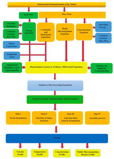
Figure 1.
Flow chart of the proposed mathematical model.
2. Governing Equations and Material
Consider the 2D steady flowing of a magnetized generalized Burgers’ nanoliquid over a stretchable surface examining the characteristics of bioconvection and moving micro-organisms across the fluid flow in the -path. The -coordinate system is taken where the -axis is along the path of the flowing, and the -axis is normal to the flowing with a stretching rapidity , as depicted in Figure 2. The magnetic field with potent is applied. The Burgers’ nanoliquid is anticipated to be a diluted suspension through a homogenous gyrotactic microbes distribution. It is to be noted that gyrotactic microbes’ swimming velocity and swimming direction are not influenced owing to the presence of nanoparticles when suspended the nanoparticles’ concentration is lower than 1%. Further assume that the bio convection impact is impelled when the suspended nanoparticles’ concentration is low. The wall is preserved at a fixed temperature and concentricity . A cooled stretched surface scenario and is taken into consideration. The concentration of species in this research is supposed to be on the high side; thus, the impacts of activation energy and bilateral reaction are considerable.
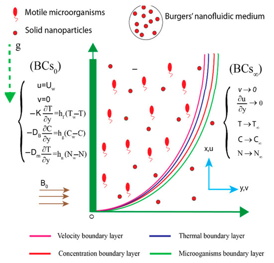
Figure 2.
Flow chart for a current problem.
Taking into account the hypotheses proposed, the regulating formulas and appropriate boundary constraints for the Burgers’ nanofluid flowing are as follows [69,70]:
having boundary conditions
The above governing equations are solved by following suitable transformations:
where , , and are functions of . The following equations are obtained:
with boundary conditions
Diverse non-dimensional factors occurring in (8)–(12) are provided below:
where , , are Deborah’s numbers, while is a parameter of the Burgers’ fluid. , and signify the magnetic field parameter, buoyancy ratio number, and Rayleigh number of bioconvection, respectively. is the Prandtl number while is utilized as a parameter for Brownian motion. is used for a different number of microorganisms whereas is a parameter for thermal radiation. and represent the Lewis number and activation energy. is the temperature difference parameter while is a chemical reaction factor. is the Lewis parameter of bio-convection and is used as the Peclet parameter. Moreover, , , , , , and signify the Biot number of heat, Biot number of solution, Biot number of microorganisms, thermophoresis parameter, relaxation parameter of heat, and parameter of mixed convection, respectively.
3. Galerkin Finite Element TechniqueGalerkin Finite Element Technique
The corresponding boundary constraints of the present system were computationally simulated using FEM. FEM is based on the partitioning of the desired region into components (finite). FEM [71] is covered in this section. Figure 3 depicts the flowing chart of the finite element technique. This procedure has been employed in numerous computational fluid dynamics (CFD) matters; the benefits of employing this strategy are discussed further below.
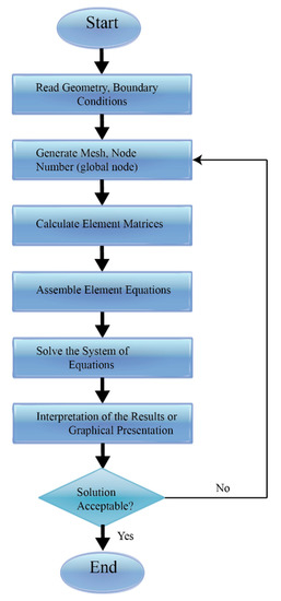
Figure 3.
Flow chart of G-FEM.
Step I: The weak form is derived from the strong form (stated ODEs), and residuals are computed.
Step II: To achieve the weak form, shape functions are taken linearly, and FEM is used.
Step III: The assembly method is used to build stiffness components, and a global stiffness matrix is created.
Step IV: Using the Picard linearizing technique, an algebraic framework (nonlinear equations) is produced.
Step V: Algebraic equations are simulated utilizing appropriate halting criterion through 10−5 (supercomputing tolerances).
Further, The Galerkin finite element technique’s flow chart is depicted in Figure 2.
4. Validity of Code
The computational technique’s authenticity was evaluated by comparing the heat transition rate from the previous methods to the authenticated results of previous research [72]. Table 1 compares the findings of the present study to the findings of the previous study. The present study is significantly compared, and the outcomes are remarkably accurate.

Table 1.
Comparison of with alteration in Prandtl number, taking and .
The important physical parameters in this problem are the local heat and mass fluxes, as well as the local motile microorganisms flux, which are specified as follows:
in which
Using the similarity transform presented above, Equation (14) can be described as follows:
5. Results and Discussion
To enhance understanding of the analysis, the results are demonstrated in tables and figures showing the impact of the thermofluid parameters on the flowing velocity, heat distribution, mass transfer, and motile microbes’ distribution. These are presented in Figure 4, Figure 5, Figure 6, Figure 7, Figure 8, Figure 9, Figure 10, Figure 11, Figure 12, Figure 13, Figure 14, Figure 15, Figure 16, Figure 17, Figure 18, Figure 19, Figure 20, Figure 21, Figure 22, Figure 23, Figure 24, Figure 25, Figure 26, Figure 27 and Figure 28 and Table 1 and Table 2 for a variational increase in the thermophysical terms. Figure 4, Figure 5, Figure 6 and Figure 7 demonstrate the material effect on flowing fluid velocity fields. A rise in dilatant Deborah number resulted in a significant decline of the nanofluid velocity magnitude as displayed in Figure 4. This is a result of enhancing shear material thickness that stimulated the bonding force. The opposed nanoparticles’ molecular interaction reduced thermal transfer, which consequently decreased the velocity distribution. Moreover, the Burgers’ nanoliquid material term increased the flow rate distribution as seen in Figure 5. The pseudoplastic term inspired Fick’s and Fourier’s thermal conductivity to boost the spinning of motile microbes along with the stretching sheet. Accordingly, the random motion of the nanoparticles was propelled, thereby encouraging the current-carrying nanofluid. As such, the flow rate past the streaming boundless medium was raised in magnitude. Likewise, the Deborah pseudoplastic number and enhanced the flow regime towards the far stream as presented in Figure 6 and Figure 7. The flow velocities were significantly raised with increasing pseudoplastic material terms. As the terms are increased, the nanoparticles’ bonding force is dominated by an internally generated heat to allow free molecular interaction of the fluid particles. Therefore, the velocity distributions were enhanced with rising Deborah numbers across the flow domain.
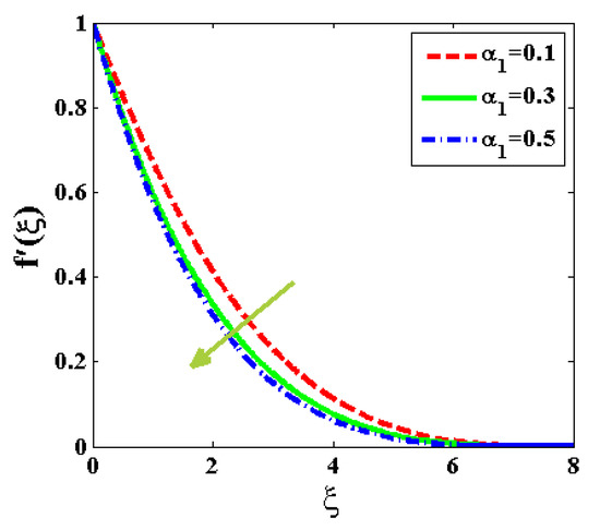
Figure 4.
Outlines of f′ at diverse quantities of .
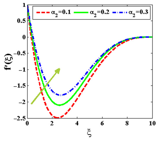
Figure 5.
Outlines of 𝑓′ at diverse quantities of .
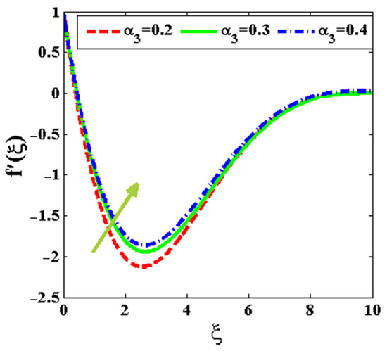
Figure 6.
Outlines of f′ at diverse quantities of .
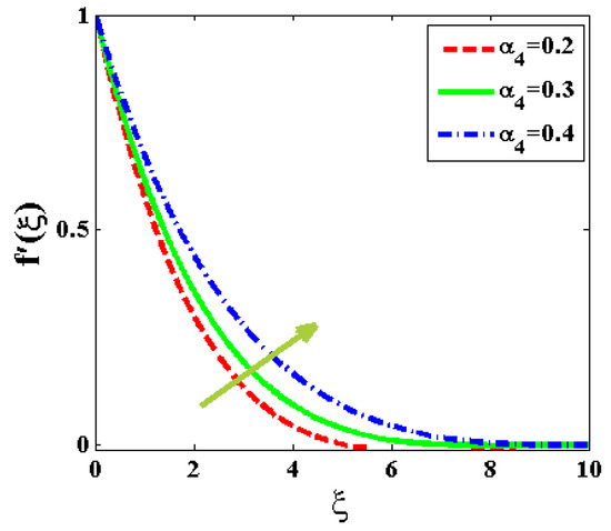
Figure 7.
Outlines of f′ at diverse quantities of .
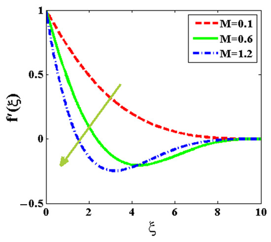
Figure 8.
Outlines of f′ at diverse quantities of .

Figure 9.
Outlines of f′ at diverse quantities of .
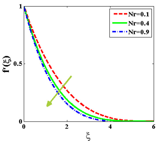
Figure 10.
Outlines of f′ at diverse quantities of .
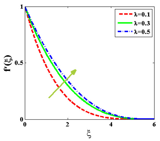
Figure 11.
Outlines of f′ at diverse quantities of .
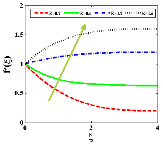
Figure 12.
Outlines of f′ at diverse quantities of .
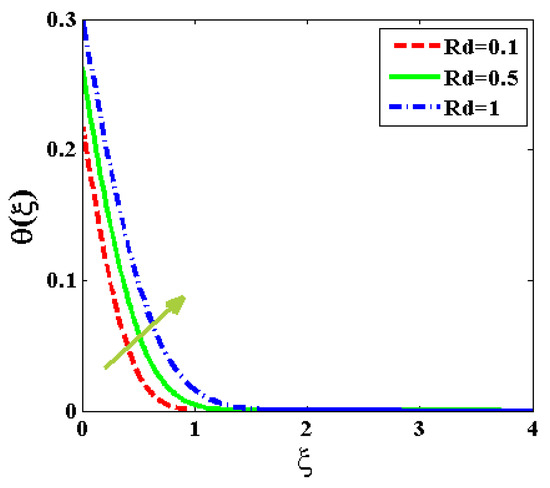
Figure 13.
Outlines of at diverse quantities of .
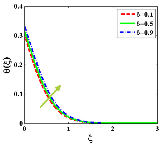
Figure 14.
Outlines of at diverse quantities of .
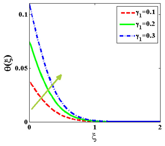
Figure 15.
Outlines of θ at diverse quantities of .
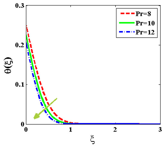
Figure 16.
Outlines of at diverse quantities of .
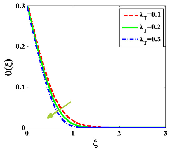
Figure 17.
Outlines of at diverse quantities of .
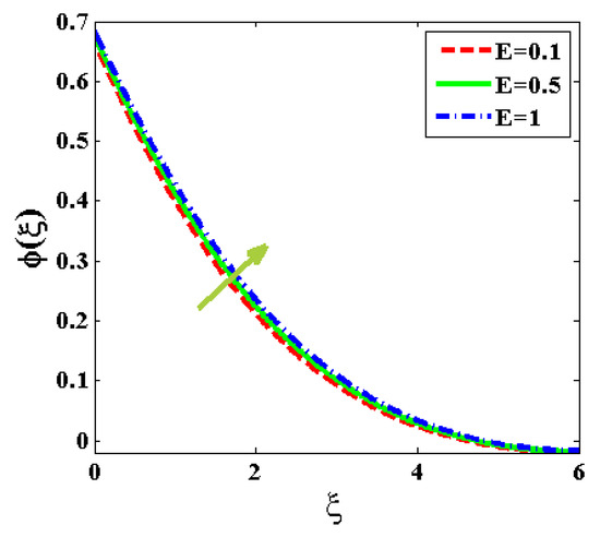
Figure 18.
Outlines of at diverse quantities of .
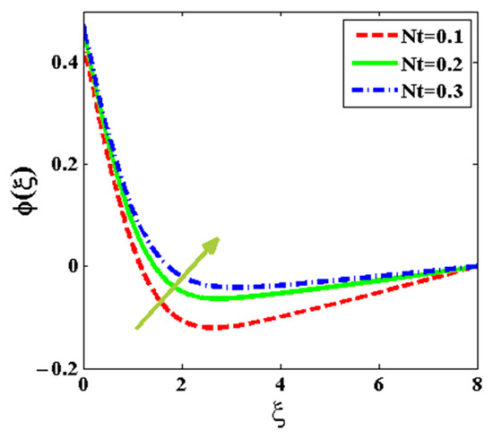
Figure 19.
Outlines of at diverse quantities of .
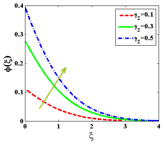
Figure 20.
Outlines of at diverse quantities of .
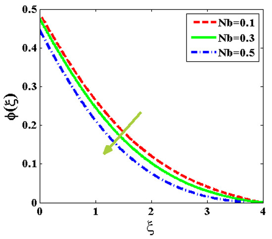
Figure 21.
Outlines of at diverse quantities of .
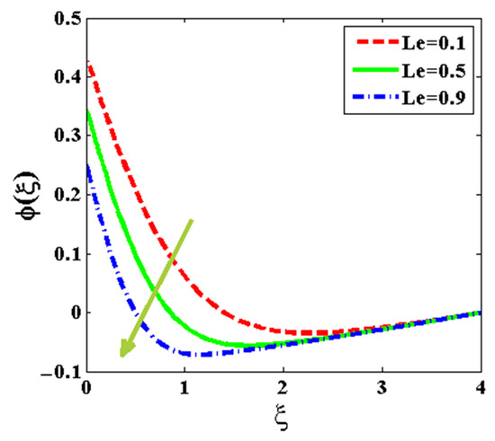
Figure 22.
Outlines of at various values of .
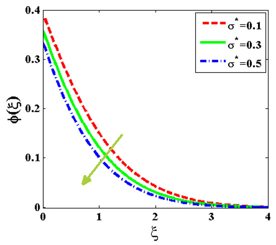
Figure 23.
Outlines of at diverse quantities of .
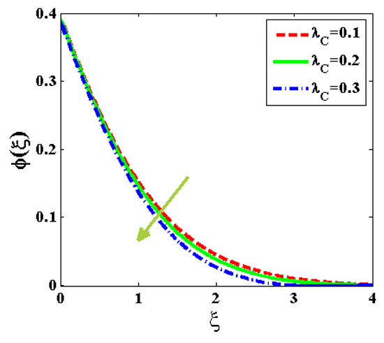
Figure 24.
Outlines of at diverse quantities of .
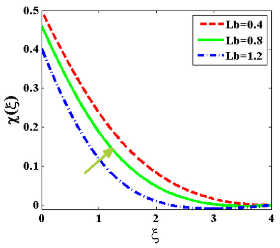
Figure 25.
Outlines of at diverse quantities of .
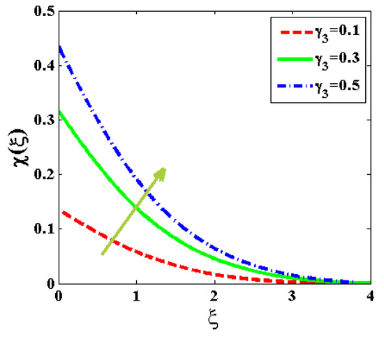
Figure 26.
Outlines of at diverse quantities of .
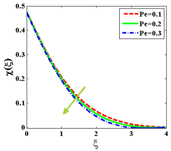
Figure 27.
Outlines of at diverse quantities of .
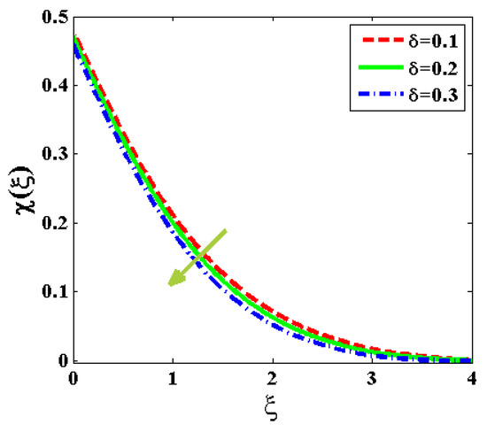
Figure 28.
Outlines of at diverse quantities of .
Table 2.
Nusselt and Sherwood quantities and consistency amount at the stretching walls.
In Figure 8, the increasing number of the magnetized force opposed the flowing velocity outline as presented. The motile microorganisms were damped due to an induced electromagnetic force that resists the nanoparticles’ free collision. This accordingly affects heat transfer, thereby meaningfully impacting the flow rate. The impact of the bioconvective Rayleigh quantity on the nanofluid flow rapidity is investigated in Figure 9. The Rayleigh number is connected with the convective buoyancy-driven flow; an increase in the Rayleigh number caused a rising flow velocity field near the stretching wall due to an enhanced heat gradient. The effect reduces along the far stream because of an increased fluid shear stress, which restricts the free flow of motile microbes. Hence, the velocity profile reduced and increased with the Rayleigh number variation. The sensitivity of the flow velocity to rising buoyancy ratio number is displayed in Figure 10. The velocity distribution was reduced as a result of the dominance of the fluid viscosity over the thermal buoyancy. As observed, the motile microorganisms of the nanofluid interaction were hampered, resulting in a significant decrease in the flow rate field. In Figure 11, the effect of increasing combined convective term on the rapidity distribution is examined. The combined natural and force convection denoting mixed convection raised the up-swimming of the microorganisms in a suspended nanoparticle, which led to an enhanced flow rate profile. The flow dimension is a result of the acted coupled convection mechanism on the Burger’s nanofluid, which propels high heat transfer past the stretched sheet. As such, the buoyancy and pressure forces interacted to boost heat propagation, which inspired the magnetized fluid velocity field. As well, in Figure 12, the parameter K significantly increased the velocity field of the motile microbes in the Burger’s nanofluid. The thermal conductivity of the fluid is stretched to create a free particle collision, thereby magnifying the velocity distribution.
Figure 13, Figure 14 and Figure 15 display the influence of the radiation term , bio-convective term and heat Biot number on the temperature distribution. The terms are a strong source of heat generation that stimulate internal heating. As observed, the heat propagation in the stretching device was boosted by the existence of Fourier and Fick thermal conductivity and low thermal diffusion. Hence, the temperature profile was increased as the nanoparticle random movement was enhanced. Therefore, in a chemical and thermal system, the terms that enhance heat transfer should be monitored to guide against chemical reaction blowup. In Figure 16 and Figure 17, The response of the heat transfer to enhancing Prandtl number and heat relaxation term is demonstrated. As noticed, the temperature field was reduced in magnitude along with the swimming motile microorganisms due to the high diffusion of heat to the environment, which was a result of a thinner energy boundary layer. The rising ambient heat dispersion reduces nanoparticles’ thermal conductivity. Hence, momentum viscosity dominates the thermal conductivity, thereby restricting Burger’s fluid molecular interaction. As such, the temperature distribution is decreased.
The effect of the thermofluid terms on the mass transfer are displayed in Figure 18, Figure 19, Figure 20, Figure 21, Figure 22, Figure 23 and Figure 24. The sensitivity of the reacting species to varying parameters is shown in the respective plots. In Figure 18, Figure 19 and Figure 20, the impression of active energy , thermophoresis term and the species Biot quantity is checked on the concentration distribution. The terms propel the solution concentration field due to the stimulation of internal energy that induced the species reaction along the boundless stream. Motile microorganism reaction close to the stretchable sheet is more noticeable than at far stream because of the rising wall thermal conductivity. Moreover, Burger’s nanofluid thermal reaction is boosted to inspire heat transfer, thereby leading to an enhanced chemical concentration distribution. In Figure 21, Figure 22, Figure 23 and Figure 24, the mass transfer diminished with a variational rise in the Brownian diffusion , Lewis number , chemical reaction term , and relaxation time . The low heat transfer through nanoparticles and motile microorganisms is due to the high molecular bond and shear stress that resists the concentration profiles. This is as well supported by the species boundary layer viscosity that supports chemical solution diffusion, thereby damping the species mass distribution. The plot of against depicting the motile microorganism distribution for parameter variations is given in Figure 25, Figure 26, Figure 27 and Figure 28. In Figure 25 and Figure 26, the impact of the bioconvective term and microorganism Biot number are examined. As is shown, the swimming microorganism distribution is increased with an enhanced parameter value because of created internal heating. The flow dimensions are due to the high-density gradient caused by the collection of convective macroscopic motion. The Biot number creates microorganism thermal resistances at the surface and inside the body to stimulate heat transfer. Therefore, the motile microbes profiled are propelled. Meanwhile, the opposite effect was obtained for the rising Peclet number and microorganism different number as seen in Figure 27 and Figure 28. The flow behavior is due to the shallow random suspensions and volume cell fraction of the motile microorganism dispersion pattern. As such, the microorganism distribution is damped in magnitude significantly.
6. Table Discussion
The numerically computed outcomes for the wall temperature gradient, mass gradient, and the motile microorganisms are presented in Table 2. The impact of different thermophysical terms has been investigated and obtained computationally. As can be seen, a rise or decline in the engineering thermofluid wall quantities could be obtained, a consequence of the thinness or thickness of the boundary layers. The boundary viscidness determines the thermal diffusion, species diffusion, and microorganism volume cell fraction. Therefore, an increase or decrease in the computed values could be obtained depicting various stretching wall effects.
7. Conclusions
The developed model describing the flow characteristics of the bioconvection and swimming microorganisms of a magnetized generalized Burgers’ nanomaterial with Fourier’s and Fick’s laws has been considered. Transformed invariant coupled quasilinear differential equations were obtained and solved using the finite element Galerkin technique via COMSOL software. The qualitative and quantitative results are provided graphically and in tables to give a clear insight into the study. The outcomes of the parameter sensitivities study are as follows:
- A significant monotonic increase in the flow velocity is seen for variations in the Rayleigh number and Deborah pseudoplastic number, and .
- A growing magnetic field term generates significant electromagnetic force, which increases shear stress and dampens the velocity profile.
- The suspended nanoparticles’ heat conduction and distribution of motile microbes are enhanced with rising radiation, bioconvective, and heat Biot number terms.
- The mass transfer and concentricity distribution are decreased for an increasing value of Brownian motion, Lewis number, and relaxation time.
- It is plausible to conclude that increasing the chemical reaction parameter and concentricity relaxation variable or reducing the Prandtl number, concentricity Biot quantity, and active energy factor can considerably enhance the concentration dispersion of nanoparticles.
- A rising value of bioconvective and microorganism Biot number spurred motile microorganism distribution.
The outcomes of this study apply to the promotion of thermal and chemical industrial productivity. As such, more investigation is encouraged along the research direction and study extension can be considered for the annular concentric cylinder flow with Arrhenius chemical kinetics. Some recent developments exploring the significance of the considered research domain are reported by [73,74,75,76,77,78,79,80,81,82].
Author Contributions
F.S. and W.J. formulated the problem. F.S., W.J., R.S. and M.R.E. solved the problem. F.S., W.J., T.S., M.S., R.S., S.O.S., M.R.E. and M.B.H. computed and scrutinized the results. All the authors equally contributed to the writing and proofreading of the paper. All authors reviewed the manuscript. All authors have read and agreed to the published version of the manuscript.
Funding
This research received no external funding.
Institutional Review Board Statement
Not applicable.
Informed Consent Statement
Not applicable.
Data Availability Statement
All data generated or analyzed during this study are included in this published article.
Conflicts of Interest
The authors declare no conflict of interest.
Nomenclature
| relaxation time parameters of Burgers’ fluid | |
| retardation time parameters of Burgers’ fluid | |
| activation energy | |
| relaxation time of heat | |
| relaxation time of mass | |
| liquid temperature | |
| liquid concentration | |
| ambient temperature | |
| ambient concentration | |
| coefficient of diffusion | |
| heat flux | |
| mass flux | |
| density | |
| pressure | |
| specific heat capacity | |
| thermal conductivity of the liquid |
References
- Bergman, T.L.; Lavine, A.S.; Incropera, F.P.; DeWitt, D.P. Introduction to Heat Transfer; John Wiley & Sons: Hoboken, NJ, USA, 2011. [Google Scholar]
- Serrano, J.; Olmeda, P.; Arnau, F.; Reyes-Belmonte, M.; Lefebvre, A. Importance of heat transfer phenomena in small turbochargers for passenger car applications. SAE Int. J. Engines 2013, 6, 716–728. [Google Scholar] [CrossRef]
- Zhang, H.; Zhuang, J. Research, development and industrial application of heat pipe technology in China. Appl. Therm. Eng. 2003, 23, 1067–1083. [Google Scholar] [CrossRef]
- Ramesh, K.N.; Sharma, T.K.; Rao, G.A.P. Latest advancements in heat transfer enhancement in the micro-channel heat sinks: A review. Arch. Comput. Methods Eng. 2021, 28, 3135–3165. [Google Scholar] [CrossRef]
- Pozhar, L.A. Structure and dynamics of nanofluids: Theory and simulations to calculate viscosity. Phys. Rev. E 2000, 61, 1432–1446. [Google Scholar] [CrossRef] [PubMed]
- Rafati, M.; Hamidi, A.A.; Niaser, M.S. Application of nanofluids in computer cooling systems (heat transfer performance of nanofluids). Appl. Therm. Eng. 2012, 45, 9–14. [Google Scholar] [CrossRef]
- Polidori, G.; Fohanno, S.; Nguyen, C.T. A note on heat transfer modelling of Newtonian nanofluids in laminar free convection. Int. J. Therm. Sci. 2007, 46, 739–744. [Google Scholar] [CrossRef]
- Huminic, G.; Huminic, A. Application of nanofluids in heat exchangers: A review. Renew. Sustain. Energy Rev. 2012, 16, 5625–5638. [Google Scholar] [CrossRef]
- Schlichting, H.; Gersten, K. Boundary-Layer Theory; Springer Science & Business Media: Berlin/Heidelberg, Germany, 2003. [Google Scholar]
- Ramadhan, A.I.; Azmi, W.H. The effect of nanoparticles composition ratio on dynamic viscosity of Al2O3-TiO2-SiO2 nanofluids. Mater. Today Proc. 2022, 48, 1920–1923. [Google Scholar] [CrossRef]
- Ramadhan, A.I.; Azmi, W.H.; Mamat, R.; Diniardi, E.; Hendrawati, T.Y. Experimental Investigation of Cooling Performance in Automotive Radiator using Al2O3-TiO2-SiO2 Nanofluids. Automot. Exp. 2022, 5, 28–39. [Google Scholar] [CrossRef]
- Seyyedi, S.M.; Hashemi-Tilehnoee, M.; Sharifpur, M. Impact of fusion temperature on hydrothermal features of flow within an annulus loaded with nanoencapsulated phase change materials (NEPCMs) during natural convection process. Math. Probl. Eng. 2021, 2021, 4276894. [Google Scholar] [CrossRef]
- Hashemi-Tilehnoee, M.; del Barrio, E.P.; Seyyedi, S.M. Magneto-turbulent natural convection and entropy generation analyses in liquid sodium-filled cavity partially heated and cooled from sidewalls with circular blocks. Int. Commun. Heat Mass Transf. 2022, 134, 106053. [Google Scholar] [CrossRef]
- Fikri, M.; Faizal, W.; Adli, H.; Bo, Z.; Jiang, X.; Ramadhan, A. Experimental Determination of Water, Water/Ethylene Glycol and TiO2-SiO2 Nanofluids mixture with Water/Ethylene Glycol to Three Square Multilayer Absorber Collector on Solar Water Heating System: A Comparative Investigation. Conf. Ser. Mater. Sci. Eng. 2021, 1062, 012019. [Google Scholar] [CrossRef]
- Malvandi, A.; Moshizi, S.A.; Soltani, E.G.; Ganji, D.D. Modified Buongiorno’s model for fully developed mixed convection flow of nanofluids in a vertical annular pipe. Comput. Fluids 2014, 89, 124–132. [Google Scholar] [CrossRef]
- Buongiorno, J. Convective transport in nanofluids. J. Heat Transf. 2006, 128, 240–250. [Google Scholar] [CrossRef]
- Kuznetsov, A.V.; Nield, D.A. Natural convective boundary-layer flow of a Nano fluid past a vertical plate. Int. J. Therm. Sci. 2010, 49, 243–247. [Google Scholar] [CrossRef]
- Tzou, D.Y. Thermal instability of nanofluids in natural convection. Int. J. Heat Mass Transf. 2008, 51, 2967–2979. [Google Scholar] [CrossRef]
- Hwang, K.S.; Jang, S.P.; Choi, S.U.S. Flow and convective heat transfer characteristics of water-based Al2O3 nanofluids in fully developed laminar flow regime. Int. J. Heat Mass Transf. 2009, 52, 193–199. [Google Scholar] [CrossRef]
- Nield, D.A.; Kuznetsov, A.V. The Cheng–Minkowycz problem for natural convective boundary-layer flow in a porous medium saturated by a nanofluid. Int. J. Heat Mass Transf. 2009, 52, 5792–5795. [Google Scholar] [CrossRef]
- Nield, D.A.; Kuznetsov, A.V. The Cheng–Minkowycz problem for the double-diffusive natural convective boundary layer flow in a porous medium saturated by a nanofluid. Int. J. Heat Mass Transf. 2011, 54, 374–378. [Google Scholar] [CrossRef]
- Khan, W.A.; Pop, I. Boundary-layer flow of a nanofluid past a stretching sheet. Int. J. Heat Mass Transf. 2010, 53, 2477–2483. [Google Scholar] [CrossRef]
- Malvandi, A.; Ganji, D.D.; Hedayati, F.; Rad, E.Y. An analytical study on entropy generation of nanofluids over a flat plate. Alex. Eng. J. 2013, 52, 595–604. [Google Scholar] [CrossRef]
- Malvandi, A.; Hedayati, F.; Domairry, G. Stagnation point flow of a nanofluid toward an exponentially stretching sheet with nonuniform heat generation/absorption. J. Thermodyn. 2013, 2013, 764827. [Google Scholar] [CrossRef]
- Malvandi, A.; Hedayati, F.; Ganji, D.D.; Rostamiyan, Y. Unsteady boundary layer flow of nanofluid past a permeable stretching/shrinking sheet with convective heat transfer. Proc. Inst. Mech. Eng. Part C J. Mech. Eng. Sci. 2014, 228, 1175–1184. [Google Scholar] [CrossRef]
- Aziz, A.; Khan, W.A. Natural convective boundary layer flow of a nanofluid past a convectively heated vertical plate. Int. J. Therm. Sci. 2012, 52, 83–90. [Google Scholar] [CrossRef]
- Sheikholeslami, M.; Gorji-Bandpay, M.; Ganji, D.D. Magnetic field effects on natural convection around a horizontal circular cylinder inside a square enclosure filled with nanofluid. Int. Commun. Heat Mass Transf. 2012, 39, 978–986. [Google Scholar] [CrossRef]
- Sheikholeslami, M.; Gorji-Bandpy, M.; Ganji, D.D.; Soleimani, S.; Seyyedi, S.M. Natural convection of nanofluids in an enclosure between a circular and a sinusoidal cylinder in the presence of magnetic field. Int. Commun. Heat Mass Transf. 2012, 39, 1435–1444. [Google Scholar] [CrossRef]
- Sheikholeslami, M.; Ganji, D.D. Heat transfer of Cu-water nano fluid flow between parallel plates. Powder Technol. 2013, 235, 873–879. [Google Scholar] [CrossRef]
- Sheikholeslami, M.; Ganji, D.D.; Ashorynejad, H.R. Investigation of squeezing unsteady Nano fluid flow using ADM. Powder Technol. 2013, 239, 259–265. [Google Scholar] [CrossRef]
- Gupta, U.; Ahuja, J.; Wanchoo, R.K. Magneto convection in a nano fluid layer. Int. J. Heat Mass Transf. 2013, 64, 1163. [Google Scholar] [CrossRef]
- Haddad, Z.; Abu-Nada, E.; Oztop, H.F.; Mataoui, A. Natural convection in nanofluids: Are the thermophoresis and Brownian motion effects significant in nanofluid heat transfer enhancement. Int. J. Therm. Sci. 2012, 57, 152–162. [Google Scholar] [CrossRef]
- Sheikhzadeh, G.A.; Dastmalchi, M.; Khorasanizadeh, H. Effects of nanoparticles transport mechanisms on Al2O3–water nanofluid natural convection in a square enclosure. Int. J. Therm. Sci. 2013, 66, 51–62. [Google Scholar] [CrossRef]
- Yacob, N.A.; Ishak, A.; Nazar, R.; Pop, I. Falkner–Skan problem for a static and moving wedge with prescribed surface heat flux in a nano fluid. Int. Commun. Heat Mass Transf. 2011, 38, 149–153. [Google Scholar] [CrossRef]
- Daungthongsuk, W.; Wongwises, S. A critical review of convective heat transfer of nanofluids. Renew. Sustain. Energy Rev. 2007, 11, 797–817. [Google Scholar] [CrossRef]
- Wang, X.-Q.; Mujumdar, A.S. Heat transfer characteristics of nanofluids: A review. Int. J. Therm. Sci. 2007, 46, 1–19. [Google Scholar] [CrossRef]
- Jamil, M.; Fetecau, C. Some exact solutions for rotating flows of a generalized Burgers’ fluid in cylindrical domain. J. Non-Newton. Fluid 2010, 165, 1700–1712. [Google Scholar] [CrossRef]
- Fetecau, C.; Hayat, T.; Khan, M.; Fetecau, C. A note on longitudinal oscillations of a generalized Burger fluid in cylindrical domains. J. Non-Newton. Fluid 2010, 165, 350–361. [Google Scholar] [CrossRef]
- Xue, C.; Nie, J.; Tan, W.C. An exact solution of start-up flow for the fractional generalized Burgers’ fluid in a porous half space. Nonlinear Analysis Theo. Math. Appl. 2008, 69, 2086–2094. [Google Scholar] [CrossRef]
- Khan, M.; Anjum, A.; Fetecau, C.; Qi, H. Exact solutions for some oscillating motion of a motions of a fractional Burgers’ fluid. Math. Comp. Mod. 2010, 51, 682–692. [Google Scholar] [CrossRef]
- Liu, Y.; Zheng, L.; Zhang, X. MHD flow and heat transfer of a generalized Burgers’ fluid due to an exponential accelerating plate with the effects of radiation. Comp. Math. Appl. 2011, 62, 3123–3131. [Google Scholar] [CrossRef][Green Version]
- Javed, M.; Hayat, T.; Alsaedi, A. Peristaltic flow of Burgers’ fluid with complaint walls and heat transfer. Appl. Math. Comp. 2014, 244, 654–671. [Google Scholar] [CrossRef]
- Awais, M.; Hayat, T.; Alsaedi, A. Investigation of heat transfer in flow of Burgers’ fluid during a melting process. J. Egyp. Math. Soc. 2015, 23, 410–415. [Google Scholar] [CrossRef]
- Bees, M.A. Advances in bioconvection. Ann. Rev. Fluid Mech. 2020, 52, 449–476. [Google Scholar] [CrossRef]
- Khan, M.; Irfan, M.; Khan, W.A.; Sajid, M. Consequence of convective conditions for flow of Oldroyd-B nanofluid by a stretching cylinder. J. Braz. Soc. Mech. Sci. Eng. 2019, 41, 116. [Google Scholar] [CrossRef]
- Tlili, I.; Waqas, H.; Almaneea, A.; Khan, S.U.; Imran, M. Activation energy and second order slip in bioconvection of Oldroyd-B nanofluid over a stretching cylinder: A proposed mathematical model. Processes 2019, 7, 914. [Google Scholar] [CrossRef]
- Waqas, H.; Shehzad, S.A.; Khan, S.U.; Imran, M. Novel numerical computations on flow of nanoparticles in porous rotating disk with multiple slip effects and microorganisms. J. Nanofluids 2019, 8, 1423–1432. [Google Scholar] [CrossRef]
- Waqas, H.; Khan, S.U.; Hassan, M.; Bhatti, M.M.; Imran, M. Analysis on the bioconvection flow of modified second-grade nanofluid containing gyrotactic microorganisms and nanoparticles. J. Mol. Liq. 2019, 291, 111231. [Google Scholar] [CrossRef]
- Khan, S.U.; Waqas, H.; Bhatti, M.M.; Imran, M. Bioconvection in the rheology of magnetized couple stress nanofluid featuring activation energy and Wu’s slip. J. Non-Equilib. Thermodyn. 2020, 45, 81–95. [Google Scholar] [CrossRef]
- Wang, Y.; Waqas, H.; Tahir, M.; Imran, M.; Jung, C.Y. Effective Prandtl aspects on bio-convective thermally developed magnetized tangent hyperbolic nanoliquid with gyrotactic microorganisms and second order velocity slip. IEEE Access 2019, 7, 130008–130023. [Google Scholar] [CrossRef]
- Waqas, H.; Khan, S.U.; Imran, M.; Bhatti, M.M. Thermally developed Falkner-Skan bioconvection flow of a magnetized nanofluid in the presence of a motile gyrotactic microorganism: Buongiorno’s nanofluid model. Phys. Scr. 2019, 94, 115304. [Google Scholar] [CrossRef]
- Khan, S.U.; Rauf, A.; Shehzad, S.A.; Abbas, Z.; Javed, T. Study of bioconvection flow in Oldroyd-B nanofluid with motile organisms and effective Prandtl approach. Physica A 2019, 527, 121179. [Google Scholar] [CrossRef]
- Li, Y.; Waqas, H.; Imran, M.; Farooq, U.; Mallawi, F.; Tlili, I. A numerical exploration of modified second-grade nanofluid with motile microorganisms, thermal radiation, and Wu’s slip. Symmetry 2020, 12, 393. [Google Scholar] [CrossRef]
- Chu, Y.M.; Khan, M.I.; Waqas, H.; Farooq, U.; Khan, S.U.; Nazeer, M. Numerical simulation of squeezing flow Jeffrey nanofluid confined by two parallel disks with the help of chemical reaction: Effects of activation energy and microorganisms. Int. J. Chem. React. Eng. 2021, 19, 717–725. [Google Scholar] [CrossRef]
- Logan, D.L. A First Course in the Finite Element Method, Cengage Learning; CL Engineering: Dbayeh, Lebanon, 2011; ISBN 978-0495668251. [Google Scholar]
- Hrennikoff, A. Solution of problems of elasticity by the framework method. J. Appl. Mech. 1941, 8, 169–175. [Google Scholar] [CrossRef]
- Courant, R. Variational methods for the solution of problems of equilibrium and vibrations. Bull. Am. Math. Soc. 1943, 49, 1–23. [Google Scholar] [CrossRef]
- CПб ЭMИ PAH. Available online: https://www.rusprofile.ru/id/3724410 (accessed on 17 March 2018).
- Hinton, E.; Irons, B. Least squares smoothing of experimental data using finite elements. Strain 1968, 4, 24–27. [Google Scholar] [CrossRef]
- Seyyedi, S.M.; Hashemi-Tilehnoee, M.; Sharifpur, M. Effect of inclined magnetic field on the entropy generation in an annulus filled with NEPCM suspension. Math. Probl. Eng. 2021, 2021, 8103300. [Google Scholar] [CrossRef]
- Hashemi-Tilehnoee, M.; Sahebi, N.; Dogonchi, A.; Seyyedi, S.M.; Tashakor, S. Simulation of the dynamic behavior of a rectangular single-phase natural circulation vertical loop with asymmetric heater. Int. J. Heat Mass Transf. 2019, 139, 974–981. [Google Scholar] [CrossRef]
- ARamadhan, I.; Basri, H.; Diniardi, E.; Almanda, D. Aplikasi Hibrida Nanofluida Di Sistem Pendingin Kendaraan Ringan Roda Empat. In Prosiding Seminar Nasional Penelitian LPPM UMJ; Universitas Muhammadiyah Jakarta (UMJ): Ciputat, Indonesia, 2021. [Google Scholar]
- Ramadhan, A.I.; Azmi, W.H.; Mamat, R. Experimental investigation of thermo-physical properties of tri-hybrid nanoparticles in water-ethylene glycol mixture. Walailak J. Sci. Technol. 2021, 18, 9335. [Google Scholar] [CrossRef]
- Ramadhan, A.I.; Diniardi, E.; Dermawan, E. Numerical study of effect parameter fluid flow nanofluid Al2O3-water on heat transfer in corrugated tube. AIP Conf. Proc. 2016, 1737, 050003. [Google Scholar]
- SAP-IV Software and Manuals. NISEE e-Library, The Earthquake Engineering Online Archive. Available online: https://nisee.berkeley.edu/elibrary/getpkg?id=SAP4 (accessed on 30 May 2022).
- Paulsen, G.; Andersen, H.W.; Collett, J.P.; Stensrud, I.T.; Trust, B. The History of DNV 1864–2014; Dinamo Forlag A/S: Lysaker, Norway, 2014; ISBN 978-82-8071-256-1. pp. 121–436. [Google Scholar]
- Strang, G.; Fix, G. An Analysis of The Finite Element Method. Prentice Hall; Prentice-Hall: Englewood Cliffs, NJ, USA, 1973; ISBN 978-0-13-032946-2. [Google Scholar]
- Zienkiewicz, O.C.; Taylor, R.L.; Zhu, J.Z. The Finite Element Method: Its Basis and Fundamentals; Butterworth-Heinemann: Oxford, UK, 2013; ISBN 978-0-08-095135-5. [Google Scholar]
- Bathe, K.J. Finite Element Procedures; Klaus-Jürgen Bathe: Cambridge, MA, USA, 2006; ISBN 978-0979004902. [Google Scholar]
- Wang, F.; Iqbal, Z.; Zhang, J.; Abdelmohimen, M.A.H.; Almaliki, A.H.; Galal, A.M. Bidirectional stretching features on the flow and heat transport of Burgers nanofluid subject to modified heat and mass fluxes. Waves Random Complex Media 2022, in press. [Google Scholar] [CrossRef]
- Ramzan, M.; Algehyne, E.A.; Saeed, A.; Dawar, A.; Kumam, P.; Watthayu, W. Homotopic simulation for heat transport phenomenon of the Burgers nanofluids flow over a stretching cylinder with thermal convective and zero mass flux conditions. Nanotechnol. Rev. 2022, 11, 1437–1449. [Google Scholar] [CrossRef]
- Qureshi, M.A. A case study of MHD driven Prandtl-Eyring hybrid nanofluid flow over a stretching sheet with thermal jump conditions. Case Stud. Therm. Eng. 2021, 28, 101581. [Google Scholar] [CrossRef]
- Jamshed, W.; Aziz, A. Entropy Analysis of TiO2-Cu/EG Casson Hybrid Nanofluid via Cattaneo-Christov Heat Flux Model. Appl. Nanosci. 2018, 8, 1–14. [Google Scholar]
- Jamshed, W. Numerical Investigation of MHD Impact on Maxwell Nanofluid. Int. Commun. Heat Mass Transf. 2021, 120, 104973. [Google Scholar] [CrossRef]
- Jamshed, W.; Nisar, K.S. Computational single phase comparative study of Williamson nanofluid in parabolic trough solar collector via Keller box method. Int. J. Energy Res. 2021, 45, 10696–10718. [Google Scholar] [CrossRef]
- Jamshed, W.; Devi, S.U.; Nisar, K.S. Single phase-based study of Ag-Cu/EO Williamson hybrid nanofluid flow over a stretching surface with shape factor. Phys. Scr. 2021, 96, 065202. [Google Scholar] [CrossRef]
- Jamshed, W.; Nisar, K.S.; Ibrahim, R.W.; Shahzad, F.; Eid, M.R. Thermal expansion optimization in solar aircraft using tangent hyperbolic hybrid nanofluid: A solar thermal application. J. Mater. Res. Technol. 2021, 14, 985–1006. [Google Scholar] [CrossRef]
- Jamshed, W.; Nisar, K.S.; Ibrahim, R.W.; Mukhtar, T.; Vijayakumar, V.; Ahmad, F. Computational frame work of Cattaneo-Christov heat flux effects on Engine Oil based Williamson hybrid nanofluids: A thermal case study. Case Stud. Therm. Eng. 2021, 26, 101179. [Google Scholar] [CrossRef]
- Jamshed, W.; Mishra, S.R.; Pattnaik, P.K.; Nisar, K.S.; Devi, S.S.U.; Prakash, M.; Shahzad, F.; Hussain, M.; Vijayakumar, V. Features of entropy optimization on viscous second grade nanofluid streamed with thermal radiation: A Tiwari and Das model. Case Stud. Therm. Eng. 2021, 27, 101291. [Google Scholar] [CrossRef]
- Jamshed, W.; Nasir, N.A.A.M.; Isa, S.S.P.M.; Safdar, R.; Shahzad, F.; Nisar, K.S.; Eid, M.R.; Abdel-Aty, A.-H.; Yahia, I.S. Thermal growth in solar water pump using Prandtl–Eyring hybrid nanofluid: A solar energy application. Sci. Rep. 2021, 11, 18704. [Google Scholar] [CrossRef]
- Jamshed, W. Finite element method in thermal characterization and streamline flow analysis of electromagnetic silver-magnesium oxide nanofluid inside grooved enclosure. Int. Commun. Heat Mass Transf. 2021, 130, 105795. [Google Scholar] [CrossRef]
- Jamshed, W.; Eid, M.R.; Hussain, S.M.; Abderrahmane, A.; Safdar, R.; Younis, O.; Pasha, A.A. Physical specifications of MHD mixed convective of Ostwald-de Waele nanofluids in a vented-cavity with inner elliptic cylinder. Int. Commun. Heat Mass Transf. 2022, 134, 106038. [Google Scholar] [CrossRef]


Publisher’s Note: MDPI stays neutral with regard to jurisdictional claims in published maps and institutional affiliations. |
© 2022 by the authors. Licensee MDPI, Basel, Switzerland. This article is an open access article distributed under the terms and conditions of the Creative Commons Attribution (CC BY) license (https://creativecommons.org/licenses/by/4.0/).