Abstract
The paper presents an application of smart measurements for establishing control network points using a Smart Station set offer by Leica. This set may provide measurements in a terrestrial surveying system and in a satellite navigation system separately or in a mixed (hybrid) use of both systems. The procedure used for creating the points was supported by two types of GNSS satellite positioning (fast static and RTK/RTN) methods and with one integrative (hybrid method realized using both terrestrial and satellite surveys) measurement method. In the results from determining the coordinates of control points using multivariate surveys (tacheometry and real-time GNSS methods), the highest differences of coordinates were no more than 0.02 m in the horizontal plane and no more than 0.04 m in vertical plane. As reference data, model coordinates of control network points determined using static GNSS occupation were used. The reference coordinates were calculated using rigorous adjustment with support of observation files from the post-processing service of the national continuously operating reference system. In accordance with the results of the study to survey the control network points in an urban environment, Smart Station equipment is used for the established geodetic data and for other engineering measurement tasks.
1. Introduction
The topic of the paper is important for all geo-activities that are related to surveying land. Globally, in geodesy, we have a control frame and, locally, we have a stated national frame; for current works, we establish networks. Progress in this term was presented in [1], which displasy the most important information for practitioners and scientists in the “Geodesy and Cartography” field of research. Nowadays, many people use the geo-data, geo-information, or some geo-portals [2], which are produced with reference to control networks. We have many methods of producing land surveying data where geodetic control points play an essential role [3]. As we know, geodetic control networks provide an established national spatial reference system [4]. In modern surveying, the geodetic data are usually realized using space (3D) data obtained from the Global Navigation Satellite Systems (GNSS) methods. Today, in GNSS positioning, six satellite navigation systems are used [5]: GPS of the United States, GLONASS of the Russian Federation, Galileo of the European Union, Compass/Beidou of China, QZSS of Japan, and IRNSS of India. The systems are used together (two or more) to increase the measurement accuracy [6,7,8]. There are more space-surveying techniques that can realize the three-dimensional geodetic data by determining or calculating the three-dimensional coordinates of surface points. The applications of geodetic control points are placed in topographic mapping [9], engineering construction measurements [10], and georeferencing survey of point clouds and raster images [11,12]. According to the classical perspective in surveying, we need reference control points to establish or check equipment (tacheometer—instrument or GNSS—receiver). In these cases, when using new sensors in surveying (UAV—photogrammetry or LIDAR—systems), the control points are helpful for guaranteeing an equal accuracy of produced geo-data [13]. In accordance with national regulation (for example in Poland with Regulation [14]), the base geodetic control network consists of points of the horizontal and the vertical networks. Nowadays, the coordinates of the horizontal (and 3D network) base geodetic control network points mainly are determined using GNSS surveying and the heights of the points are usually determined using geometric precise leveling. The base geodetic control network points are stations of the continuously operating reference system (CORS in Poland named ASG-EUPOS), which established the three-dimensional geodetic data. In the ASG-EUPOS reference network, the average error of the point’s position should not exceed 0.01 m and the error of the point’s height should not be greater than 0.02 m.
Generally, in geodesy and especially in surveying topics, the classical method of new applications and modern configurations is used. Photogrammetric flights (raids) for land survey are realized using unmanned aerial vehicles (UAV) from low-altitude distances [15]. Triangulation (directions measurements) may be represented using laser scanning technology [16]. The idea of GNSS surveying can be equated with the implementation of the geodetic intersection task, because the satellite navigation systems are similar to the land-based systems where the satellites act as the reference points [17]. Nowadays, the innovation concept of direct land surveying is the smart station survey, including integrated tacheometric measurements using real-time GNSS positioning, e.g., by Leica [18]. The technology of the smart station surveying was defined by the trends in economic and measurement activity too [19]. Over the last few decades, some innovations in land surveying have been implemented, for example, in establishing the control networks [20,21]. Initially, GPS techniques (currently GNSS technologies) help to eliminate the need for the highest (first) order control point densification and improve the accuracy of control network points [22,23]. Nowadays, first order control network points are created in accordance with the EUPOS standard for national CORS; the following assumptions were made: existing EPN and IGS stations have been incorporated into the network of reference stations and the mean distance between stations is 70 km. Moreover, the locations of the reference stations were chosen to ensure convenient conditions for GNSS satellite observations and only precise dual-frequency GNSS receivers have been used.
Typically, the estimation of the accuracy of the network horizontal and vertical points are specified with respect to an appropriate national geodetic datum [24]. The tasks involving constructing control network points will most often need to know the position’s relationship to the realization of the reference frame [25]. Constructing control networks is a huge challenge that individual countries and research centers are working on. Previously, the horizontal geodetic control networks were established using triangulation and traversing or using photogrammetry methods, while the vertical geodetic control networks were established using geometric leveling. For example, we know the standards and specifications for geodetic control networks from the United States of America [26]. Today, Global Navigation Satellite Systems and GNSS methods are generally used to establish both horizontal and vertical control network points. In this process, some tasks must be resolved, including planning of observation [27], and precise point positioning and calculation in the aspect of the solution of the fixed points [28,29,30].
2. Materials and Methods
During the application of a smart station survey for establishing control network points, three measurement methods were performed. The procedure for point positioning was supported by performing two satellite GNSS measurement methods (fast static and RTK/RTN GNSS positioning) and one integration (hybrid method realized by terrestrial and satellite positioning) surveying method.
The reference materials in the research are coordinates (X, Y, and Z) of nine control points established using GNSS static occupation over three days with three sessions every day [31]. The static sessions were started at 8 a.m., 10 a.m., and 12 a.m.—in three parts each day, with points measured in different sessions. The control network points were situated in the area of the University of Warmia and Mazury in Olsztyn in various field conditions on the Kortowo campus (Figure 1).
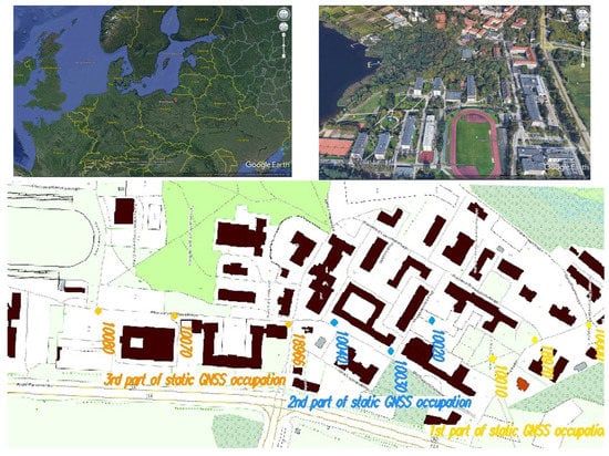
Figure 1.
Localization of analyzed control network points on the Kortowo campus.
The points were determined using static occupation over 90 min with the recording interval set to 30 s and a 10-degree elevation mask using three Topcon HyperPro GPS/GLONASS receivers. For post-processing purposes, the reference data were obtained from nearby permanent stations (BART, DZIA, ILAW, KROL, LAMA, and OLST) using the ASG-EUPOS POZGEO D service [32]. Rigorous adjustment was realized in the procedure dedicated for 3D and GNSS networks with the use of C-GEO software from Softline company [33], in the coordinate reference system EPSG:2178 (name PL-2000, Poland CS2000 zone 7), and in the geoid-based vertical system PL-KRON86-NH. Reference (model) coordinates for the control network points with accuracy were appointed: horizontal errors mXY ≤ 0.004 m and vertical mZ ≤ 0.003 m.
The model data were used for calculating the differences of coordinates after applying reference (r) GNSS static occupation and with the use of an individual (i) measurements scenario (the steps of the proposed approach are presented below in Figure 2).
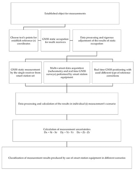
Figure 2.
A diagram with the proposed approach and the evaluation parameters used in work.
After calculating the measurement uncertainties, we may classify the surveying results and proposed measuring equipment for position and height determination in the centimeter range. According to professional practice with real-time GNSS positioning, for typical cases: high-quality engineering surveys in monitoring and construction works, with uncertainties DXY < 0.01 m and DZ < 0.02 m; basic engineering surveys and real estate surveying, with uncertainties DXY < 0.03 m and DZ < 0.05 m; civil engineering surveys, with uncertainties DXY and DZ no greater than 0.20 m; and surveying tasks in natural boundaries, with uncertainties DXY and DZ no greater than 0.50 m are all used. Similar national CORS guidelines [32] in this regard state that the estimated precision of real-time surveying is 0.03 m (horizontally) and 0.05 m (vertically).
The performed measurements were the inspiration for defining the following main aims of this study:
- (1)
- Checking the possibilities of replacing full static GNSS surveys using the single receiver measurement.
- (2)
- A multi-variant data acquisition for reference point stationing from surveys performed using smart station equipment.
- (3)
- Investigation of the used impact’s type of reference corrections on the real-time GNSS positioning of the control network points.
In the study of the method with the use of static surveys with a single receiver from the smart station set, analyses were performed of the coordinates of the control points hat were determined by the static occupation over 30 min with different recording intervals set to 1, 5, 10, 15, and 30 s and a 10-degree elevation mask using Leica GS15 receiver. The detailed analyses were mainly realized for the interval sets recorded with 1 and 5 s; this was due to practical recommendations for short static measurements carried out as part of the national satellite positioning system [32]. The differences between the coordinates calculated from the reference coordinates from the model static GNSS occupation and the results of the post-processing from the single receiver static survey were analyzed. The analyses considered fifteen scenarios of measurements marked in this key, for example: 1 s G&GL mean 1 s interval of recording GPS and GLONASS signals, 10s G mean 10 s interval of recording only GPS signals, and 30 s GL mean 30 s interval of recording only GLONASS signals.
The multi-variant measurements of control network points were realized as traversing. In the study, analyses of the coordinates of the control points that were determined using total angular–linear measurements and RTK/RTN surveys using the Leica Smart Station set were performed. The angles and distances were surveyed using the Leica TS15 tacheometer; it was a robotic total station that measured with accuracy: directions 1″ (0.0003 gon) and distances 1 mm + 1.5 ppm (in standard mode), while a Leica GS15 receiver was used for the real-time technique surveying (in VRS, MAC and SRS corrections).
In the next study, analyses of the coordinates of the control points that were determined using only RTK/RTN surveys with a Leica GS15 receiver were performed. The real-time technique was realized by using multiple reference stations (VRS or MAC) and single reference station (SRS) corrections. Some points were located in more difficult field conditions, in the so-called “city canyons”, under trees, and near buildings. The Kortowo campus is a wonderful place for the study of activity [34]. In our geo-engineering activities, we carry out many measurement works on the campus. We designate control network points for direct surveys and checkpoints for remote measurement techniques and their location was also the subject of previous publications by poster or paper [35,36].
3. Results
The typical analyses of various methods of surveying are based on differences of coordinates. In the presented analyses, the coordinates produced using full static GNSS surveys were stated as references. The results of the studies carried out in our own research, previously [35], currently, and within the framework of the diploma studio were used [31].
3.1. Results of Static Surveys Using a Single Receiver from Smart Station Set
In the case of static surveys using a single receiver from a smart station set, the differences between reference coordinates from model static GNSS occupation and the results from single receiver were considered. The calculated differences from the model static GNSS coordinates and the results of the post-processing from the single receiver static survey are present below in Figure 3a–i.
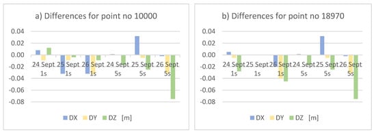
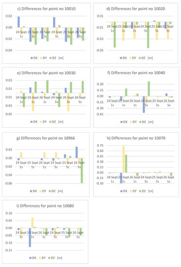
Figure 3.
Differences of coordinates between reference coordinates from model static GNSS occupation and rapid static surveys (in subfigures a–i are presented differences in meters with commas as decimal signs).
Additionally, Dilutions of Precision (DOP) parameters and root mean square (RMS) errors of analyzed scenarios of measurements were considered. In accordance with the literature [37] in science and engineering, the probability density curve is often of a particular shape known as a normal distribution (the Gaussian law of errors). To quantify such a distribution or dispersion of possible errors with a single number, we use the standard deviation (σ). We can determine σ experimentally by using a large number of observations and calculating the square root of the sum of the squares of the errors in the observations divided by one less than the number of observations (n). It is a method of computing σ as the RMS error with a probability of 68.3% [37], for example, in the case of X coordinate, . When researching a three-dimensional position (using X, Y, and Z coordinates), . Generally, satellite positioning accuracy is measured using the combined effect of the unmodeled measurement errors of pseudo-range (σ) and the effect of satellite geometry (DOP). The Dilutions of Precision can be measured using a single non-dimensional coefficient, where a low DOP coefficient represents a better positional precision due to the wider angular reparative between the satellites used to calculate a user’s position. So, the lower the value of this coefficient, the better the geometric strength and vice versa [30]. The various DOP forms are used [38]; the Geometric Dilution of Precision (GDOP) coefficient determines the multiplication factor of the estimation of total position and time errors. The Horizontal Dilution of Precision (HDOP represent the contribution to the 2D positioning accuracy) , the Vertical Dilution of Precision (VDOP represent the contribution to the altitude accuracy) , and the Position Dilution of Precision (PDOP represents the contribution of the satellite geometry to the 3D positioning accuracy) . The extreme value of the DOP and RMS for realized scenarios of measurements were stated and the results are presented in Table 1.

Table 1.
The extreme value of DOP and RMS for different scenarios of rapid static surveys.
Today’s surveyors are more interested in the concept of the maximum error, which varies from 95% to the 99% probability limits [39]. For the post-processing accuracy estimation of fast static GNSS surveying, in accordance with technical characteristics of the typical satellite receivers [40]: ±3 mm + 0.5 ppm × D for horizontal (Hz) component and ±5 mm + 0.5 ppm × D for vertical (V) component, where D is the distance to the nearest reference station were used.
In analyses considering standard uncertainty, both horizontal and vertical components are accounted for together (about 68% probability) . Multiply by a coverage factor (k) an use the fairly standard coverage factor of 3 too, which provides a coverage probability (confidence level) of approximately 99%. The coverage factor k = 3 multiplied by the standard uncertainty is termed expanded uncertainty U99 for a position, considering both horizontal and vertical components together (3D), and is written as .
The expected accuracy for the scenario of the rapid static surveys of nine measurement points were calculated and the results are presented in Table 2.
Table 2.
Expected accuracy of rapid static GNSS surveys.
The range of RMS errors from the characteristics of post-processing calculation (Table 1) matches well with the expected accuracy assessing the uncertainty interval calculated for horizontal and vertical components together U68(3D)–U99(3D) (uncertainty approximated with confidence level from 68% to 99%, in Table 2).
3.2. Results of Multi-Variant Surveys Performed Using Smart Station Equipment
In the case of multi-variant surveys, the differences of coordinates were calculated too. The differences between the reference coordinates from model static GNSS occupation and the surveys performed using smart station equipment were calculated. The number of maximum differences in positioning (for plus or minus) after applying GNSS static occupation and with the use of the individual type of corrections in multi-variant measurements (single reference station SRS, master-auxiliary concept MAC, or virtual reference station VRS). The number of extreme differences (NoED) of coordinates between the reference coordinates from model static GNSS occupation and surveys performed using the smart station are present below in Figure 4.
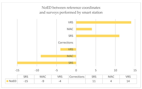
Figure 4.
Number of maximum differences in positioning after applying GNSS static occupation and with use the individual type of corrections in multi-variant measurements.
The detailed differences of coordinates (DX, DY, and DZ) were also considered and the stated results are presented below in Table 3.
Table 3.
Differences of coordinates after applying GNSS static occupation and with use of the individual type of corrections in multi-variant measurements.
For classical accuracy estimation of the multi-variant data acquisition for reference point stationing, rigorous adjustment was realized. The parameters and results of the adjustment of terrestrial and satellite surveys performed using smart station equipment are presented in Table 4.
Table 4.
Results of rigorous adjustment of terrestrial and satellite surveys performed using smart station equipment in multi-variant measurements.
The obtained RMSE from adjustment in the horizontal and vertical plane (shown in the last two rows of Table 4) are close to the differences present in Table 3. The characteristics for the terrestrial measurements obtained a posteriori are approximate to the assumed errors a priori. It is different for GNSS vectors surveying in fast static procedure, where the average errors were calculated from a variance–covariance matrix. It has been previously found in the literature [41] that, in the case of GPS (today GNSS), the rapid static positioning of the formal variance–covariance matrix output using processing software is of little use.
3.3. Results of RTK/RTN Surveys
The calculated differences of the coordinates between the reference coordinates from the model static GNSS occupation and of RTK/RTN surveys performed using the GNSS receiver from a smart station set are presented below in Figure 5. The number of extreme differences (NoED) of coordinates between the reference coordinates from the model static GNSS occupation and surveys performed using RTK/RTN GNSS are presented below in Figure 5.
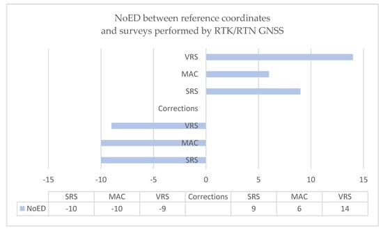
Figure 5.
Number of maximum differences in positioning after applying GNSS static occupation and with use the individual type of corrections in RTK/RTN surveys.
The detailed differences of coordinates (DX, DY, and DZ) and the minimal and maximal values of the differences stated in the real-time techniques were considered and are presented in Table 5.
Table 5.
Differences of coordinates after applying GNSS static occupation and with the use of real-time technique measurements.
In accordance with the adopted recommendations [40], for accuracy estimation of the real-time GNSS positioning, the following characteristics were used: ±8 mm + 1 ppm × D for the horizontal (Hz) component and ±15 mm + 1 ppm × D for the vertical (V) component, where D is the distance to the nearest reference station. The expected accuracy for the scenario of the real-time technique measurements of nine measurement points were also calculated and the results are presented below in Table 6.
Table 6.
Expected accuracy of real-time GNSS surveys.
It can be noticed that, if the total of differences of coordinates (DX, DY, and DZ) presented in Table 5 are included, the range would be obtained that corresponds fairly well with the expected accuracy assessing the uncertainty interval calculated for the horizontal and vertical components together U68(3D)–U99(3D) (uncertainty approximated with confidence level from 68% to 99%, in Table 6).
4. Discussion
The possibility of utilizing the GNSS surveys for object navigation and geodetic measurements are dependent on its positioning accuracy, which is strictly related to the number of satellites forming the constellation [42]. In accordance with the literature [43], using two satellite systems (GPS and GLONASS) significantly increases the accuracy of measurements.
The results from determining the coordinates of the control points using the static surveys method with a single receiver stated, for all calculation variants, that the error in the position of the point in the horizontal plane (DXY) did not exceed 0.03 m and, quite abnormally, was twice as large as the error in determining the point in the vertical plane (DZ). In general, the largest differences in coordinates (calculated from reference coordinates) were obtained for the adjustment using only one system (GPS), while the minimum differences in the coordinates were found for the solution using observations from both systems (GPS and GLONASS).
In the considered scenarios of the measurements, the biggest difference for the X coordinate equal to 0.160 m was obtained for point 10030 (30 s GL). However, the smallest difference for the X coordinate equal to 0.000 m was obtained for point 10070 (30 s G&GL). The biggest difference for the Y coordinate equal to 0.170 m was obtained for point 10030 (15 s GL). However, the smallest difference for the Y coordinate equal to 0.000 m was obtained for points: 10000 (5 s G&GL), 18970 (5 s GL, 10 s GL, and 15 s GL), 10020 (15 s G&GL, 15 s G), 18966 (15 s G&GL and 30 s G&GL), and 10070 (15 s G&GL). The biggest difference for the height (for Z coordinate), equal to 0.248 m, was also found for point 10030 (30 s GL). On the other hand, the smallest difference for the Z coordinate equal to 0.000 m was obtained for points: 10020 (30 s G&GL) and 10080 (1 s G&GL).
The results from determining the coordinates of the control points using the multi-variant survey method stated that the highest number of maximum coordinate differences from the reference coordinates were obtained for the total angular–linear and RTK/RTN measurements assumed on the basis of corrections from the virtual reference stations (VRS corrections). On the other hand, the most measurement results close to the reference coordinates were obtained for the multi-variant surveys with corrections from a single station (SRS).
In detail, the biggest difference for the X coordinate equal to −0.018 m was obtained for point 10030 (VRS). However, the smallest difference for the X coordinate equal to 0.002 m was obtained for point 10000 (SRS). The biggest difference for the Y coordinate equal to −0.013 m was obtained for point 10080 (SRS). However, the smallest difference for the Y coordinate equal to 0.000 m was obtained for points: 10020 (SRS), 10030 (MAC and SRS), 10040 (SRS), 18966 (MAC), and 10070 (MAC). The biggest difference for the height (for Z coordinate), equal to −0.038 m, was obtained for point 10080 (VRS). On the other hand, the smallest difference for the Z coordinate equal to −0.001 m was obtained for point 10030 (SRS).
In the results from the method establishing control network points by using RTK/RTN surveys, the greatest number of measurement results close to the reference coordinates were obtained for the MAC corrections and for the height for corrections from a single station (SRS).
The highest number of maximum coordinate differences was obtained for the control network points established on the basis of corrections from the virtual reference stations (VRS corrections), while the number of minimum coordinate differences was very similar for all types of corrections.
In detail, the biggest difference for the X coordinate equal to −0.031 m was obtained for point 10030 (VRS). However, the smallest difference for the X coordinate equal to 0.002 m was obtained for the following points: 18970 (SRS), 18966 (VRS), and 10080 (MAC and VRS). The biggest difference for the Y coordinate equal to 0.024 m was obtained for point 10040 (VRS). However, the smallest difference for the Y coordinate equal to 0.000 m was obtained for points: 10030 (SRS) and 10070 (VRS). The biggest difference for the height (for Z coordinate), equal to −0.059 m, was obtained for point 10010 (VRS). On the other hand, the smallest difference for the Z coordinate equal to −0.005 m was obtained for point 10030 (MAC).
In Figure 4 and Figure 5, the frequency of the minimum and maximum differences after applying GNSS occupation using the individual types of corrections are displayed (SRS, MAC, or VRS). The minimal differences in coordinates were practically even for SRS, MAC, and VRS corrections. However, the maximal differences in the coordinates were stated for VRS correction, in contrast to MAC correction, which is in accordance with the literature [44]. It is also practically correct that the high-quality solution was obtained for positioning with the use of a single reference station (SRS correction).
The performed studies did not show any significant difference in the results of the measurements using the GPS system or the GLONASS system. Of course, with the use of both systems (GPS and GLONASS), the number of satellites in the constellation was bigger and the accuracy of positioning of control network points was, therefore, also higher. It was especially noticeable at the points located in more difficult field conditions (near trees and buildings); these are the control points numbered: 10040, 10070, and 10080. Generally, for the control network points that were determined by 30 min sessions of static occupation, the differences of coordinates (X, Y, and Z) to the reference coordinates were no more than 0.030 m. Some of the results of the presented investigations are not very typical, as they were probably influenced by the time window of the satellite positioning and the approximately north–south orientation of the sequence of measured points. For example, the environments of points 10040 and 10070 are relatively poor, but these points have even better results than the other points (see Figure 3). In accordance with the literature [45], the urban environment is characterized by the presence of an excessive number of obstacles that produce a multipath effect in the positioning of the GNSS receiver.
Additional assessments were also used in the paper, for results of GNSS positioning were applied in assessing the expected accuracy [40]. The uncertainty interval calculated for the horizontal and vertical components together corresponds quite well with those presented in this work of the differences of the coordinates. When they are totally included, these could represent the displacement distance (as a vector obtained from DX, DY, and DZ in a three-dimensional Cartesian system). In the case of multi-variant surveys (terrestrial and satellite hybrid measurements) the observations were adjusted using a classical approach [46]. The available publications also present the results of a further integration of satellite positioning and terrestrial measurements [47,48].
5. Conclusions
In this paper, the application of a smart station survey for creating control network points was presented. As we know from the United States Patent (No. 5,233,357 and Date: 3 August 1993) Smart Station set offered by Leica, results may be obtained using measurements in a terrestrial surveying system and in satellite navigation system separately or in mixed-use (hybrid) systems [49].
The calculated differences of the coordinates between the reference coordinates from the model static GNSS occupation, the results of post-processing from single receiver static surveys as well as from RTK/RTN surveys performed using a GNSS receiver, and, finally, multi-variant surveys performed using smart station equipment were considered.
The results for determining coordinates of control points using the multi-variant survey method (tacheometry and real-time GNSS methods) stated that the highest differences of coordinates were no more than 0.02 m in the horizontal plane (uncertainty DXY) and no more than 0.04 m in the vertical plane (uncertainty DZ).
After using real-time GNSS occupation, the differences of the coordinates were no more than 0.03 m in the horizontal plane (DXY) and no more than 0.06 m in the vertical plane (DZ). Certainly, the high accuracy of the kinematic measurement using SRS correction is influenced by the fact that the used single reference station was located a short distance from the research area (less than 2 km). The network measurement with MAC correction has an interpolation algorithm, which provides greater possibilities and independence from the need to “trust” to VRS correction [44].
With the use of multi-variant surveys realized using Smart Station angular–linear and RTK/RTN measurements, a weaker solution was obtained on the basis of the corrections from the virtual reference station (VRS correction). The most measurement results close to the reference coordinates were obtained for the multi-variant surveys with corrections from a single reference station (SRS).
Nevertheless, the research results have shown that the use of Smart Station equipment is very hopeful for measuring urban environments, establishing control network points, and for other purposes (in areas with no full GNSS signals, e.g., near trees and buildings). This is in accordance with the results presented in the research of other authors [50].
Funding
This research was funded by the Department of Geodesy, University of Warmia and Mazury in Olsztyn, Poland, statutory research no. 29.610.001-110.
Institutional Review Board Statement
Not applicable.
Informed Consent Statement
Not applicable.
Data Availability Statement
Research data is available in the author’s archive.
Acknowledgments
Thanks to the Head Office of Geodesy and Cartography in Poland for main source of the provided data and GNSS real-time corrections, and for Colleagues and Students cooperating in measurement works.
Conflicts of Interest
The author declares no conflict of interest.
References
- Scientific Assembly of the International Association of Geodesy (IAG). Abstract Book; IAG: Beijing, China, 2021. [Google Scholar]
- Lists of Geoportals. University of Texas Libraries. Available online: https://guides.lib.utexas.edu/gis/lists-of-gis-data-portals (accessed on 7 May 2022).
- Doskocz, A. The current state of the creation and modernization of national geodetic and cartographic resources in Poland. Open Geosci. 2016, 8, 579–592. [Google Scholar] [CrossRef]
- Lu, Z.; Qu, Y.; Qiao, S. Geodesy—Introduction to Geodetic Datum and Geodetic Systems; Springer: Berlin/Heidelberg, Germany, 2014. [Google Scholar] [CrossRef]
- Camacho-Lara, S. Current and Future GNSS and Their Augmentation Systems. In Handbook of Satellite Applications; Pelton, J.N., Madry, S., Camacho-Lara, S., Eds.; Springer: New York, NY, USA, 2013; pp. 617–654. [Google Scholar] [CrossRef]
- Montenbruck, O.; Steigenberger, P.; Hauschild, A. Multi-GNSS signal-in-space range error assessment—Methodology and results. Adv. Space Res. 2018, 61, 3020–3038. [Google Scholar] [CrossRef]
- Wu, Z.; Wang, Q.; Yu, Z.; Hu, C.; Liu, H.; Han, S. Modeling and performance assessment of precise point positioning with multi-frequency GNSS signals. Measurement 2022, 201, 111687. [Google Scholar] [CrossRef]
- Ashour, I.; El Tokhey, M.; Mogahed, Y.; Ragheb, A. Performance of global navigation satellite systems (GNSS) in absence of GPS observations. Ain Shams Eng. J. 2022, 13, 101589. [Google Scholar] [CrossRef]
- Oki, S. Control Point Surveying and Topographic Mapping. In Civil Engineering Vol. I; Kiyoshi Horikawa, K., Qizhong Guo, Q., Eds.; UNESCO, Encyclopedia of Life Support Systems: Paris, France, 2009; pp. 158–172. [Google Scholar]
- Sztubecki, J.; Topoliński, S.; Mrówczyńska, M.; Bagrıaçık, B.; Beycioglu, A. Experimental Research of the Structure Condition Using Geodetic Methods and Crackmeter. Appl. Sci. 2022, 12, 6754. [Google Scholar] [CrossRef]
- Otepka, J.; Ghuffar, S.; Waldhauser, C.; Hochreiter, R.; Pfeifer, N. Georeferenced Point Clouds: A Survey of Features and Point Cloud Management. ISPRS Int. J. Geo-Inf. 2013, 2, 1038–1065. [Google Scholar] [CrossRef]
- Oniga, V.-E.; Breaban, A.-I.; Pfeifer, N.; Chirila, C. Determining the Suitable Number of Ground Control Points for UAS Images Georeferencing by Varying Number and Spatial Distribution. Remote Sens. 2020, 12, 876. [Google Scholar] [CrossRef]
- What Is Geodata? A Guide to Geospatial Data. Available online: https://gisgeography.com/what-is-geodata-geospatial-data (accessed on 4 June 2022).
- Regulation of the Minister of Development, Labor and Technology of 6 July 2021 on Geodetic, Gravimetric and Magnetic Control Networks. Journal of Laws of 2021, Item 1341 (in Polish), with Information in English. Available online: https://www.geoportal.gov.pl/en/dane/osnowy-podstawowe (accessed on 18 January 2023).
- Pyka, K.; Wiącek, P.; Guzik, M. Surveying with Photogrammetric Unmanned Aerial Vehicles. Arch. Photogramm. Cartogr. Remote Sens. 2020, 32, 79–102. [Google Scholar] [CrossRef]
- Emam, S.M.; Khatibi, S.; Khalili, K. Improving the accuracy of laser scanning for 3D model reconstruction using dithering technique. Procedia Technol. 2014, 12, 353–358. [Google Scholar] [CrossRef]
- GPS, GNSS and Geodesy Concepts. North Group LTD. Available online: https://www.northsurveying.com/index.php/soporte/gnss-and-geodesy-concepts (accessed on 24 May 2022).
- Biasion, A.; Cina, A.; Pesenti, M.; Rinaudo, F. An integrated GPS and Total Station instrument for cultural heritage surveying: The Leica Smartstation example. In Proceedings of the CIPA XX International Symposium: International Cooperation to Save the World’s Cultural Heritage, Torino, Italy, 26 September–1 October 2005; CIPA Organising Committee: Torino, Italy, 2005; pp. 13–18. [Google Scholar]
- Brouwer, T.; Koeva, M.; van Oosterom, P.; Theunisse, I. Smart Surveyors: Developments and Trends from the FIG Working Week 2020. Available online: https://www.gim-international.com/content/article/smart-surveyors (accessed on 17 February 2022).
- Dąbrowski, W.; Dorzak, A. The perspectives for the development of reproducible network technology based on 12 years of experience. Sci. J. Agric. Univ. Wroc. 1997, 14, 99–112, (In Polish with English Summary). [Google Scholar]
- Gargula, T. Research on geometrical structure of modular networks. Geod. Cartogr. 2004, 53, 189–202. [Google Scholar]
- Bałandynowicz, J.; Dąbrowski, W.; Gąsowska, B. Restorable networks strengthened by GPS vectors. Geod. Cartogr. Vilnius Tech. 2000, XXVI, 116–122. [Google Scholar]
- Gargula, T. The conception of integrated survey networks composed of modular networks and GPS vectors. Surv. Rev. 2009, 41, 301–313. [Google Scholar] [CrossRef]
- Dąbrowski, J. Accuracy Standards of Tying the Horizontal and Vertical Control Network to the National Geodetic Control Network. Geomat. Environ. Eng. 2014, 8, 41–57. [Google Scholar] [CrossRef]
- Wolski, B.; Granek, G. Functionality and reliability of horizontal control net (Poland). Open Geosci. 2020, 12, 668–677. [Google Scholar] [CrossRef]
- Bossler, J.D. Standards and Specifications for Geodetic Control Networks; Federal Geodetic Control Committee: Silver Spring, MD, USA, 1984. [Google Scholar]
- Mehrabi, H.; Voosoghi, B. Optimal observational planning of local GPS networks: Assessing an analytical method. J. Geod. Sci. 2014, 4, 87–97. [Google Scholar] [CrossRef]
- Kurt, O.; Konak, H.; Ince, C.D. The design and evaluation stages of local GPS networks for monitoring crustal movements. In Proceedings of the Conference Papers of International Earthquake Symposium, Kocaeli, Turkey, 17–19 August 2009. [Google Scholar] [CrossRef]
- Wielgosz, P.; Paziewski, J.; Baryła, R. On Constraining Zenith Tropospheric Delays in Processing of Local GPS Networks with Bernese Software. Surv. Rev. 2011, 43, 472–483. [Google Scholar] [CrossRef]
- Januszewski, J. Sources of Error in Satellite Navigation Positioning. Int. J. Mar. Navig. Saf. Sea Transp. 2017, 11, 419–423. [Google Scholar] [CrossRef]
- Stasiak, P.A.; Szczepkowski, M. Geodetic Control Points Performer with Smart Station Technology. Master’s Thesis, University of Warmia and Mazury, Olsztyn, Poland, 2014. (In Polish). [Google Scholar]
- Services of the Multifunctional Precise Satellite Positioning System ASG-EUPOS Offered in Poland and a Compendium of Knowledge on the Practical Aspects of GNSS Measurements. Available online: http://www.asgeupos.pl/index.php?lng=EN (accessed on 24 August 2022).
- Information About C-GEO Software Offer by Softline. Available online: http://www.c-geo.com (accessed on 24 August 2022). (In English).
- Information About Kortowo Campus. Available online: http://www.uwm.edu.pl/en/study-at-uwm/kortowo-campus (accessed on 24 May 2022).
- Doskocz, A.; Uradziński, M. Determination of control network points by Smart Station technology using correction from ASG-EUPOS service. In Proceedings of the Conference of Sections the Control Networks and the Earth’s Dynamic from Committee of Geodesy in Polish Academy of Sciences 2011. Poster sessions, Warsaw–Józefosław, Poland, 17–18 October 2011. (In Polish). [Google Scholar]
- Doskocz, A.; Uradziński, M. Position determination of control network points in the Smart Station technology using ASG-EUPOS system. Rep. Geod. 2012, 92, 155–162. [Google Scholar]
- Langley, R. The Mathematics of GPS. GPS World 1991, 2, 45–50. [Google Scholar]
- Langley, R. Dilution of Precision. GPS World 1999, 5, 52–59. [Google Scholar]
- Specht, M. Statistical Distribution Analysis of Navigation Positioning System Errors—Issue of the Empirical Sample Size. Sensors 2020, 20, 7144. [Google Scholar] [CrossRef] [PubMed]
- Manandhar, D. Interpreting GNSS Specifications. United Nations Office for Outer Space Affairs, Presentation 2021. Available online: https://www.unoosa.org/documents/pdf/icg/2021/Tokyo2021/ICG_CSISTokyo_2021_19.pdf (accessed on 30 November 2022).
- Han, S.; Rizos, C. Standarization of the variance-covariance matrix for GPS rapit static positioning. Geomat. Res. Australas. 1995, 62, 37–54. [Google Scholar]
- Specht, C.; Mania, M.; Skóra, M.; Specht, M. Accuracy of the GPS positioning system in the context of increasing the number of satellites in the constellation. Pol. Marit. Res. 2015, 22, 9–14. [Google Scholar] [CrossRef]
- Specht, C.; Koc, W. Mobile satellite measurements in designing and exploitation of rail roads. Transp. Res. Procedia 2016, 14, 625–634. [Google Scholar] [CrossRef]
- Janssen, V. A comparison of the VRS and MAC principles for network RTK. In Proceedings of the International Global Navigation Satellite Systems Society IGNSS Symposium 2009, Surfers Paradise, QLD, Australia, 1–3 December 2009. [Google Scholar]
- Titouni, S.; Rouabah, K.; Atia, S.; Flissi, M.; Khababa, O. GNSS multipath reduction using GPS and DGPS in the real case. Positioning 2017, 8, 47–56. [Google Scholar] [CrossRef]
- Welsch, W.M. Problems of accuracies in combined terrestrial and satellite control networks. J. Geod. Former. Bull. Géodésique 1986, 60, 193–204. [Google Scholar] [CrossRef]
- Niemeier, W.; Tengen, D. Uncertainty assessment in geodetic network adjustment by combining GUM and Monte-Carlo-simulations. J. Appl. Geodesy 2017, 11, 67–76. [Google Scholar] [CrossRef]
- Gargula, T. Adjustment of an Integrated Geodetic Network Composed of GNSS Vectors and Classical Terrestrial Linear Pseudo-Observations. Appl. Sci. 2021, 11, 4352. [Google Scholar] [CrossRef]
- 100 Years Innovation HEERBRUGG. United States Patent for SmartStation Set Offer by Leica. p. 200. Available online: https://www.flipsnack.com/hexagongeo/100-years-innovation-heerbrugg-hexagon-anniversary-book/full-view.html (accessed on 17 February 2022).
- Cheng, H.; Xi, G.; Ke, F.; Zhen, L.; Wei, G.; Fei, Y. Application and Study of Smart Station for Special Environment and Real Time Localization. In IEEE Conference Publication, Proceedings of the 2010 International Conference on Multimedia Technology, Ningbo, China, 29–31 October 2010; IEEE: New York, NY, USA, 2010. [Google Scholar] [CrossRef]
Disclaimer/Publisher’s Note: The statements, opinions and data contained in all publications are solely those of the individual author(s) and contributor(s) and not of MDPI and/or the editor(s). MDPI and/or the editor(s) disclaim responsibility for any injury to people or property resulting from any ideas, methods, instructions or products referred to in the content. |
© 2023 by the author. Licensee MDPI, Basel, Switzerland. This article is an open access article distributed under the terms and conditions of the Creative Commons Attribution (CC BY) license (https://creativecommons.org/licenses/by/4.0/).