Article

Retinex-Based Relighting for Night Photography

Nagoya Institute of Technology, Nagoya 464-8602, Japan
*
Author to whom correspondence should be addressed.
Appl. Sci. 2023, 13(3), 1719; https://doi.org/10.3390/app13031719
Submission received: 8 December 2022 / Revised: 24 January 2023 / Accepted: 26 January 2023 / Published: 29 January 2023
(This article belongs to the Special Issue Advances in Digital Image Processing)

Abstract

:
The lighting up of buildings is one form of entertainment that makes a city more colorful, and photographers sometimes change this lighting using photo-editing applications. This paper proposes a method for automatically performing such changes that follows the Retinex theory. Retinex theory indicates that the complex scenes caught by the human visual system are affected by surrounding colors, and Retinex-based image processing uses these characteristics to generate images. Our proposed method follows this approach. First, we propose a method for extracting a relighting saliency map using Retinex with edge-preserving filtering. Second, we propose a sampling method to specify the lighting area. Finally, we composite the additional light to match the human visual perception. Experimental results show that the proposed sampling method is successful in keeping the illuminated points in bright locations and equally spaced apart. In addition, the proposed various diffusion methods can enhance nighttime skyline photographs with various expressions. Finally, we can add in a new light by considering Retinex theory to represent the perceptual color.

1. Introduction

Lighting up buildings is a form of entertainment that adds color to cities. This lighting can be physically changed, but it is not easy to change the lighting on a building after taking a photograph of it. After the image is captured, photographers can change the lighting of the photo by using photo-editing applications, such as Adobe Photoshop. However, creating illuminated photography manually is a time-consuming and challenging task.
In this paper, we automatically generate and change the illuminated light in an image based on the Retinex theory [1,2,3], which is based on the human visual system (HVS). Generally, colors in images are determined by interactions between lights and illuminated surfaces. This interaction depends on the reflectivity and shape of the subject. Therefore, we should analyze this information to create natural lighting; however, understanding this information from photographs alone is a complex problem.
Retinex theory shows that HVS does not perceive absolute brightness but rather relative brightness, capturing the brightness perceived simultaneously with the ambient brightness. There are various multimedia applications based on this relation: low-light enhancement [4,5,6,7,8,9,10], high-dynamic range imaging [11], haze removal [12,13], underwater image enhancement [14], shadow removal [15], denoising [16], medical imaging [17,18], and face recognition [19].
Low-light enhancement is the application most related to the proposed method. For the enhancement of low-light images, one method is to emphasize very dark areas by accurately separating the illumination from the reflected light. Because of the multiplicative nature of the illumination and reflectance relationship, poor estimation accuracy for one will result in worse accuracy for the other. Recent approaches [5,6,7,8,20] solve this problem using complex solutions. While early studies for low-light enhancement are computationally lightweight, the reflectance component is directly separated from the illumination and regarded as the enhanced output, which often causes over-enhancement [4]. Current algorithms [5,6,7,8,20] estimate the illumination and reflectance components by adding the prior constraints, and then they obtain the enhanced low-light image by multiplying the reflectance component with the adjusted illumination component.
Our research target is relighting nighttime skyline shots as a new multimedia application using Retinex theory. The difference in our approach from low-light enhancement is the dynamic range required for the final image. Low-light enhancement requires a wider dynamic range to make dark areas visible, while our application only requires a narrow dynamic range since only bright areas will change illumination, not dark areas, limiting the number of re-lit regions. Thus, the transformation of illuminated intensity can be restricted to a linear transformation instead of a non-linear one. The final image can be directly transformed with the linear transformation from the input image and illuminating the color map in the Lab color space. The additional illuminating color map in the final image is artificial; thus, the map does not require an estimation of the original physical illumination. Our method estimates only perceptual reflectance, which indicates the additional illuminating location. Only a rough shape, such as an edge, is needed to estimate reflectance; thus, our approach is lightweight and does not cause significant degradation.
Our approach has three steps. First, we generate the reflectance field using single-scale Retinex (SSR) [21], and then the reflectance is convoluted by min-filtering and joint bilateral filtering [22,23]. All filters can be a O(1) constant-time property for each filtering radius: min-filtering [24], Gaussian filtering [25], and joint bilateral filtering [26]. Recent low-light enhancement approaches [5,6,7,8,20] assume that an inverted low-light image looks like a hazy image, and the inverted image can be enhanced via the haze-removal approach [27]. With this flow, they use min-filtering and guided image filtering [28,29] as an edge-preserving filter as an analogy to the proposed method. Second, we generate several light source points on the reflectance field based on a probabilistic model with blue noise sampling, which is often used in computer graphics [30]. Next, we generate light shapes based on various spread functions with or without edge-preserving factors. Finally, we relight photographs using the input images and generated illuminating factors.  Figure 1 presents an overview of the proposed flows. The main contributions are as follows:
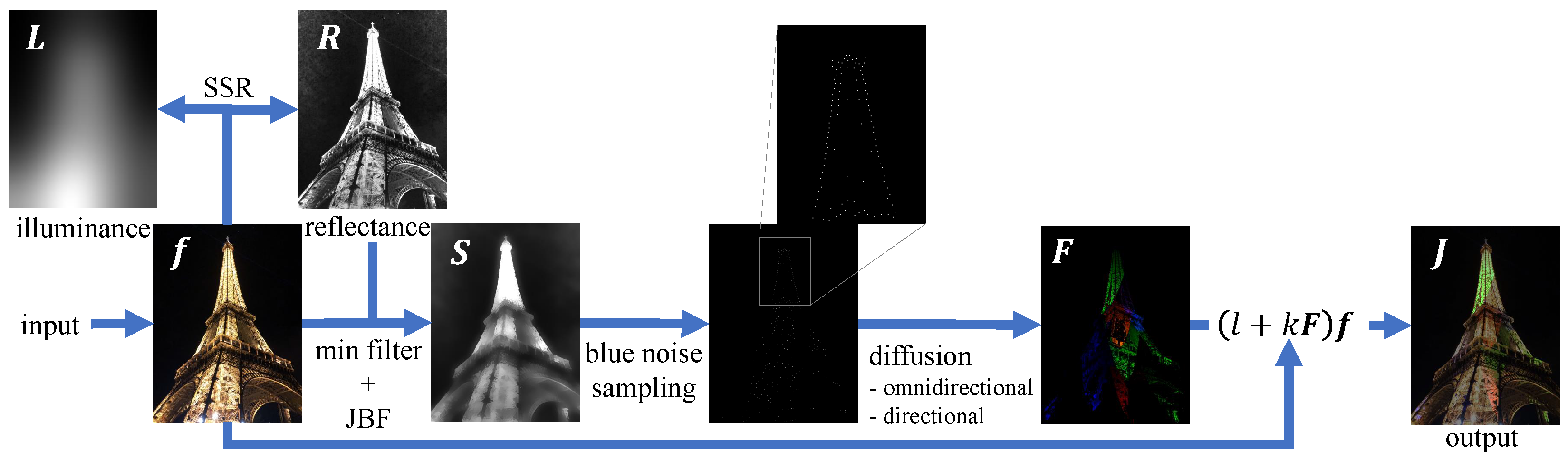
  • We propose a new Retinex-based application of relighting night photography, i.e., changing illumination based on the HVS.
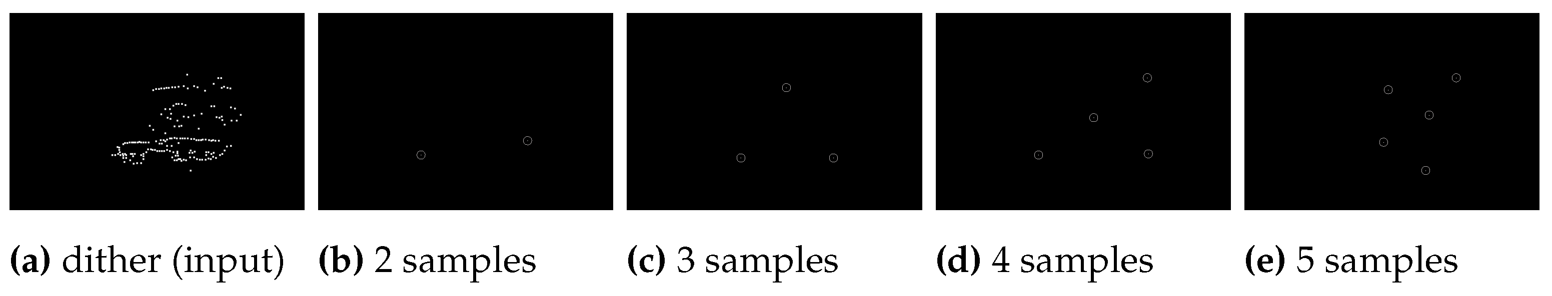
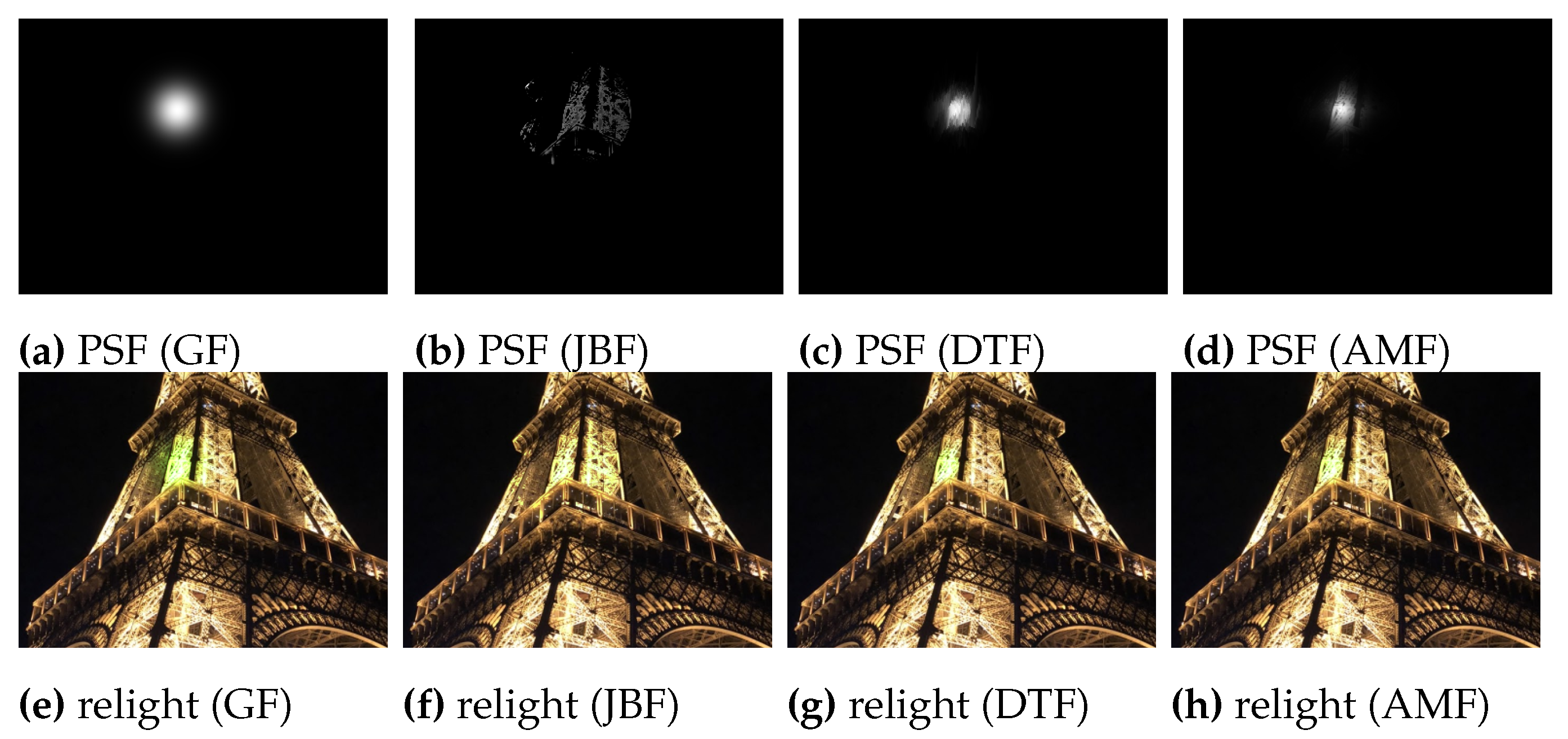
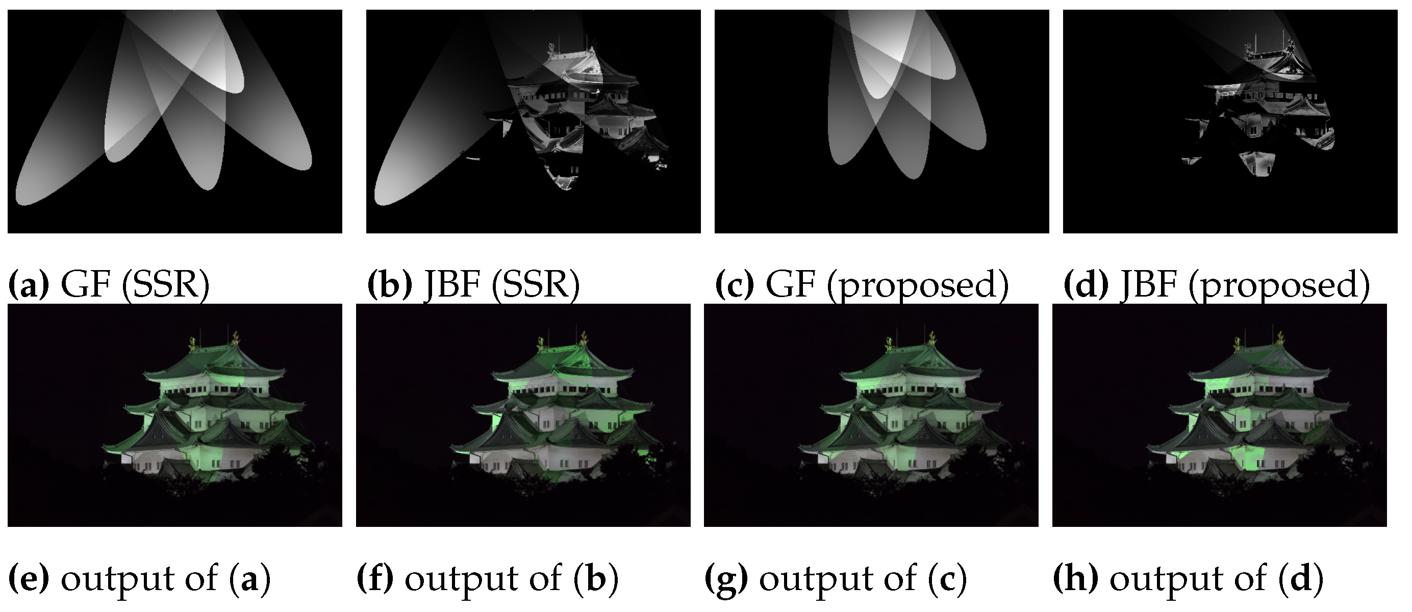
  • We propose a light source sampling method based on blue noise sampling, which is used in computer graphics. In addition, we propose various light shape generation methods: a point spread function with or without an edge-preserving factor and a hyperbola function to produce a searchlight effect (i.e., a directional light to illuminate a certain location).
  • We propose a method with a constant time property for the convolution radius. The independency is realized by using constant time filters in all processes in our method.
Figure 1. Overview of the proposed method.
Applsci 13 01719 g001

2. Retinex Theory

2.1. Overview

Land introduced the Retinex theory in 1964 to model how the HVS perceives a scene [1]. The HVS does not perceive absolute brightness but rather relative brightness. The fundamental observation is the insensitivity of human visual perception to a slowly varying illumination in a Mondrian-like scene. Recent reviews are presented in [31,32]. However, the goal has since shifted toward reflectance–illumination decomposition, which is picked up from the Retinex model.
There are various approaches to the decomposition problem of illumination and reflectance: threshold-based (PDE) Retinex [33,34], reset-based (random walk) Retinex [35], center-surround Retinex [3,21,36,37], and variational Retinex [31,38,39], and more recently, convolutional neural networks used for Retinex [40,41]. In another context, this separation is called intrinsic image decomposition [42,43,44,45], where the intrinsic image is the reflectance image in the Retinex.
The Retinex model involves the idea that the captured image f is the product of an illumination map L and a reflectance map R of the object [46]. It is defined as follows:
f = L R ,
where the operator ⊙ indicates the Hadamard product. The reflectance R is the intrinsic feature of the observed scene, which is not affected by the illumination component L as the extrinsic property. We can measure f but not directly capture L and R . All symbols used in this paper are reviewed in Appendix A.

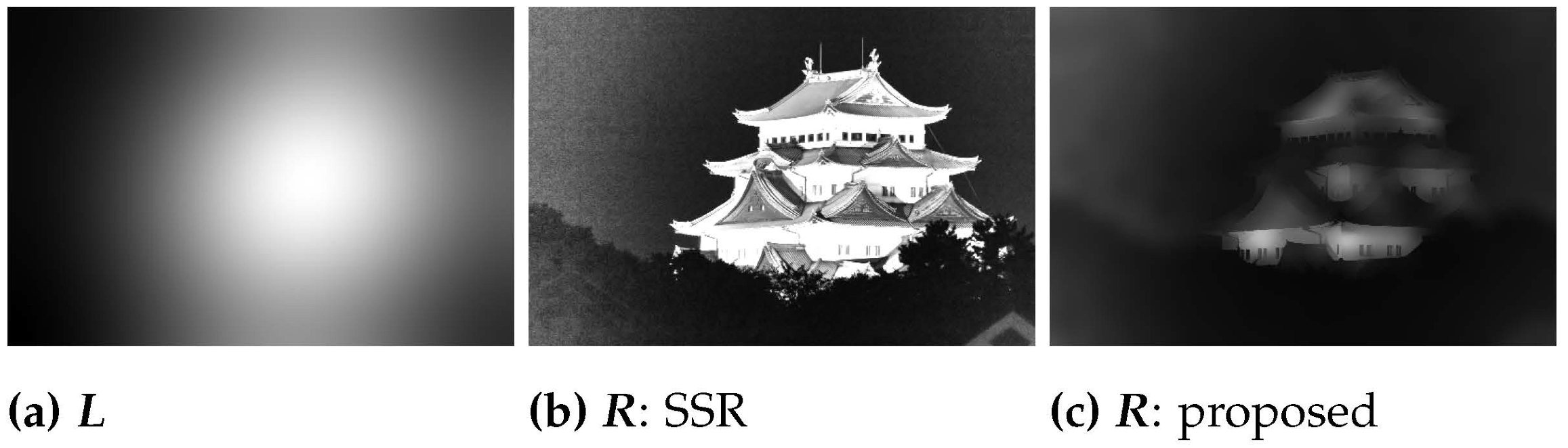
2.2. Single-Scale Retinex

Land introduced the center/surround Retinex [3]. It is based on the idea that brightness is calculated as the ratio of the value of a pixel to the mean value of the surrounding points and that these surrounding points have a density proportional to the inverse of the squared distance. This operation is similar to high-pass filtering, and Jobson et al. applied it using the Gaussian convolution [21,36,37]. Here, we define one version of this filter called single-scale Retinex (SSR). Smoothing filters can compute the surrounding field on each pixel, such as the mean of the neighboring pixels for mean filtering.
Let a D-dimensional, B-tone image be f : S R , where S R D is the spatial domain, R [ 0 , B 1 ] d is the range domain, and d is the color range dimension (generally, D = 2 , B = 256 , and d = 3 ), respectively. The SSR output image, which is the reflectance, R : S R , is defined by
R p = f p g f p ,
where p S is a pixel position. Equation (2) is based on the center-surrounding model of Retinex theory [21,36,37]. f p and R p are intensity vectors of the input and output images, respectively. The operator ∗ indicates a convolution, and here, we use Gaussian filtering (GF) as a traditional SSR representation defined by
g f p = q Ω p exp p q 2 2 2 σ 2 f q q Ω p exp p q 2 2 2 σ 2 ,
where Ω p S is the set of the neighboring pixels of p and σ is a smoothing parameter for the Gaussian distribution. Equation (2) means that the algorithm satisfies color constancy.
In SSR, a higher σ results in an output image with better color fidelity but a lower dynamic range. A smaller σ leads to an enhanced dynamic range but greater color distortion. For better balancing, the multi-scale Retinex (MSR) is also introduced [36]; however, MSR requires complex parameter tuning [47]. The simpler SSR was used because there is no need to consider the color distortion of the reflectance in this paper, as will be discussed later.

3. Proposed Method

This paper proposes an algorithm that partially relights nighttime skyline photographs and determines the positions and shapes of light sources. The proposed method has four steps: (1) extracting an illuminating saliency map, (2) sampling lighting points from the saliency map as a 2D probability distribution, (3) diffusing the lighting points for generating omnidirectional/directional lighting area, and (4) relighting based on Retinex enhancement. The following sections describe the detailed information for each step.

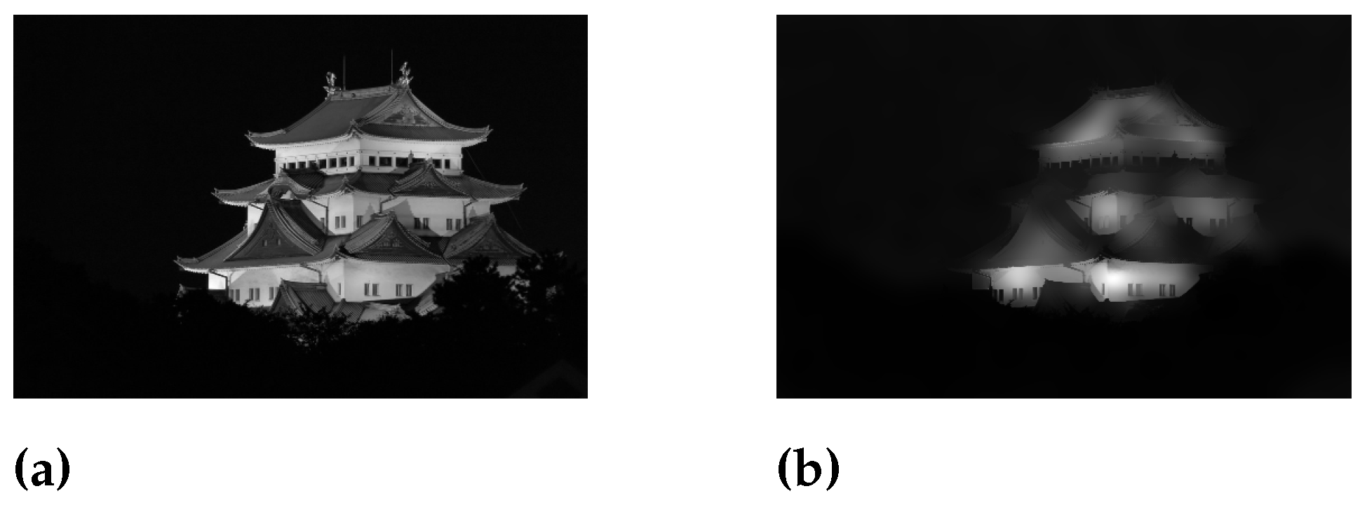
3.1. Illuminating Saliency Map

For illuminating images, lighting source points should be in human–visual saliency areas. The well-known saliency map [48] indicates that the human eyes focus on distinctive areas in the natural scene. For relighting night photography, we assume that the light source points should be located in high-reflectance areas. Therefore, the saliency map for this relighting is based on the reflectance map.
A simple solution uses reflectance images directly. However, there are some half pixels due to blurring or object boundaries. When the new lighting point is in a mixed area, lights spread across both foreground and background objects. Therefore, we erode the reflectance image and diffuse it using edge-preserving filtering to avoid this problem.
First, we convert the image to grayscale and apply SSR to extract the salient light areas in the input image. Examples of input color and grayscale images, L , and R from SSR are shown in  Figure 2,  Figure 3a, and  Figure 3b, respectively. To compute SSR, we use a sliding-DCT-based convolution [25,49,50,51], which has a constant-time property per pixel for convolution. The FFT computational order is O ( log N ) per pixel, where N is the number of image pixels, while that of sliding-DCT is O ( 1 ) . SSR is known to produce white shadows near the boundaries of objects, i.e., halo artifacts. The halo causes problems in the next step of dithering. Therefore, we erode the reflectance area to extract the more pronounced light component without the halo effect by min-convolution and iterative joint bilateral filtering (JBF) [22,23].
Next, we erode the reflectance image R , which is defined as follows:
R p min = inf q Ω p min R q ,
where Ω p min is a set for the convolution area, also called min-convolution. We use OpenCV’s implementation, which is O ( 1 ) order per pixel and is based on recursive filtering [24].
After the min-convolution, we diffuse the processed reflectance map using an iterative version of JBF. JBF is a variant of bilateral filtering (BF) [52], and the difference between BF and JBF is only the guidance signal for measuring color distance. BF measures the color distance for kernel weight from the filtering target of the input signal, while JBF measures it from an additional guide signal. Let the guide signal be the input f and the t-th iterative input and output signal be S p t and S p t + 1 , respectively. Iterative JBF is defined by
S p t + 1 = q Ω p jbf w s ( p , q ) w r ( f p , f q ) S q t q Ω p jbf w s ( p , q ) w r ( f p , f q ) ,
where S 1 = R min , w s : S × S R is a spatial kernel, and w r : R × R R is a range kernel. The kernels are based on the Gaussian distribution:
w s ( p , q ) = exp q p 2 2 2 σ s 2 , w r ( f p , f q ) = exp f q f p 2 2 2 σ r 2 ,
where σ s R + is a spatial scale and σ r R + is a range scale. We denote the final output as S = S t + 1 , where t is the number of JBF iterations, and we normalize S from 0 to 1 for the next step. The resulting output is shown in Figure 3c. Note that we accelerate JBF based on the constant-time BF [26,53] with the constant-time GF. GF, min-convolution, and JBF are constant for the filtering radius. That is, all processing is a constant time for each filtering radius.
Figure 4a, which is multiplied by SSR as a reflectance image (Figure 3b) and uses the GF image as an illuminance image (Figure 3a), is completely the same as  Figure 2 in grayscale. In comparison, Figure 4b, which is multiplied by R of the proposed method (Figure 3c) and using the GF image (Figure 3c), is not the same as the input image, as shown in  Figure 2. However, this is not a problem since this R is not used for the final output.

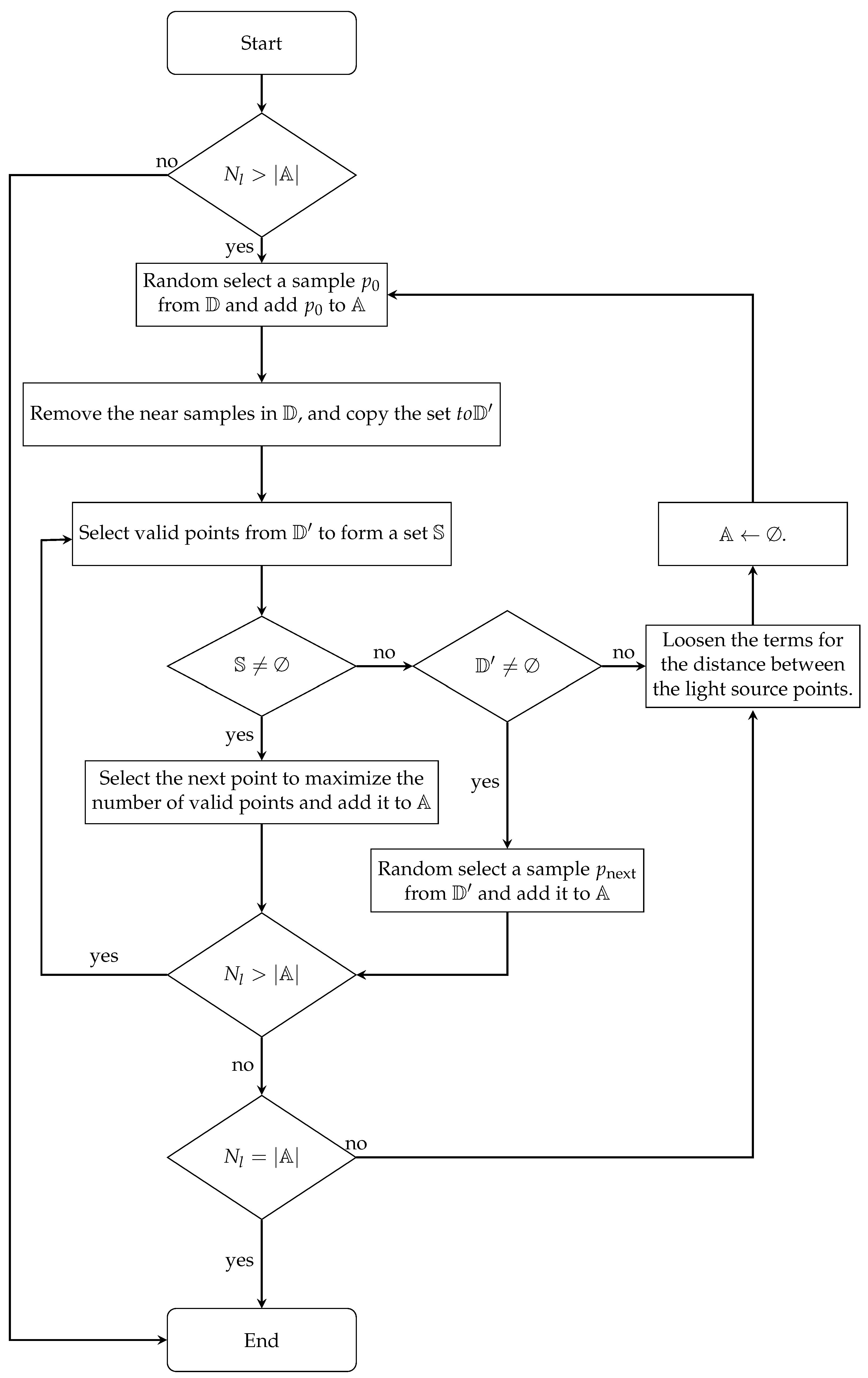
3.2. Lighting Points Sampling

We select N light source points based on S as a 2D probability distribution, where the normalized saliency map is S p [ 0 , 1 ] 1 . In addition, the samples must have a greater distance from each other, called blue noise sampling [30]. This paper introduces an efficient sampling method from S with dithering and blue noise sampling.
First, we use dithering S to extract the candidates of samples. Dithering is a blue noise sampling method [54,55]; however, it cannot control the number of samples. To change the number of samples, intensity remapping for dithering has been proposed [56]. Ideally, in dithering, the number of samples is the summation of the probability; N = S . Thus, a remapping function for S can control the number of samples. Lou et al. [56] used the clipping linear function U ( h , v ) = min ( h x , 1 ) . Given the desired number of samples N d , the input S is remapped and dithered to obtain the appropriate samples by setting the most suitable v that satisfies equation N d = U ( S , v ) . The detailed information is shown in [56]. Note that the number of sampling points N d is not the final number. We regard the dithering samples as candidates’ points because dithering does not have randomness, i.e., fixed samples. Therefore, we select the final sampling points from the dithered samples, i.e., oversampled dithering samples. An example of the dithering output is shown in  Figure 5a.
After performing remapped dithering, the oversampled points N d are randomly resampled based on blue noise sampling to reduce the number of the last samples N l . This task is equivalent to selecting light sources from N d . In the selection process, the distance between the points should be as far apart as possible to illuminate a wide area.
The resampling is performed according to  Figure 6 and Algorithm 1. First, we select a point randomly at lines 5 and 6 in Algorithm 1. Next, we find a point that has a distance within the range r l and maximum distance γ r l from the already sampled points while maximizing the remaining points that can be sampled as much as possible, which is shown in line 7 to line 23. Then, we iterate the sampling process. If the condition is not met, we retry the process by reducing r l to make it easier to meet the condition that is represented from lines 24 to 26. After processing, we can select the light source point set of A from the dithering point set D , where the number of samples is N l = | D | .  Figure 5 shows examples of the proposed sampling method. All points are sampled at a certain distance and at approximately equal intervals.
Algorithm 1: Sample light source from dithering points
Applsci 13 01719 i001

3.3. Diffusing Lighting Source Points

To define the illuminating area from the sampling points, we propose two types of diffusion: omnidirectional and directional. Omnidirectional diffusion is based on the point spread function (PSF) of filtering. Directional diffusion uses a rotated hyperbolic function to represent searchlight-like lighting, a cropped set of an omnidirectional PSF. The two types of diffusion are used according to how we want to render the image.
Let a PSF for the n-th sampling point be P n : S [ 0 , 1 ] 1 , i.e., normalized 0 to 1 in grayscale. The illuminating color map F : S [ 0 , B 1 ] 3 ( B = 256 ) is the product sum of each PSF and user-specific color vectors and is defined as follows:
F p = n A P p n C n ,
where A is the set of light source points and C n R 3 is a user-determined color vector (3 channels) for the n-th sampling point, e.g., red [ 255 , 0 , 0 ] , green [ 0 , 255 , 0 ] , and blue [ 0 , 0 , 255 ] . The following describes PSF generation methods for omnidirectional and directional diffusion.

3.3.1. Omnidirectional Diffusion

First, we explain omnidirectional diffusion. A primary method of omnidirectional diffusion uses the PSF of Gaussian filtering (GF). This kernel spreads light evenly in all directions. However, PSF of GF is not a sufficient method because it produces light outside of the target object. Therefore, we additionally use the PSF of edge-preserving filters: JBF, domain transform filtering (DTF) [57], and adaptive manifolds filtering (AMF) [58]. The PSF of edge-preserving filters depends not only on a spatial kernel, such as GF, but also on a range kernel. The kernel of joint edge-preserving filtering using the input image as a guide image can suppress light diffusion at the object boundary of the reflectance guide.
For the range kernel, JBF uses a Gaussian distribution with the Euclidean distance defined in Equation (6). The DTF range kernel uses the geodesic distance of image edges instead of the Euclidean distance, and the AMF range kernel uses the mixed Euclidean–geodetic distance. The core ideas are defined as follows:
w r DTF ( f p , f q ) = exp f q f p geo 2 2 σ r 2 , w r AMF ( f p , f q ) = exp f q f p mix 2 2 σ r 2 ,
where · geo indicates geodesic distance and · mix indicates the mixed Euclidean–geodetic distance. The geodesic distance considers changes in the value along the path. The definition is as follows:
f p f q geo = p q | f o | d o ,
where f o is a differential value along the path from p to q and | · | is the absolute function. The mixed Euclidean–geodetic distance is the blended value between Euclidean and geodetic distances:
f p f q mix = blend ( f p f q geo , f p f q )
where blend is a blending function. The actual response is different from these functions because of the approximation processes: separable approximation and range value approximation. See the papers [57,58] for the actual definitions.

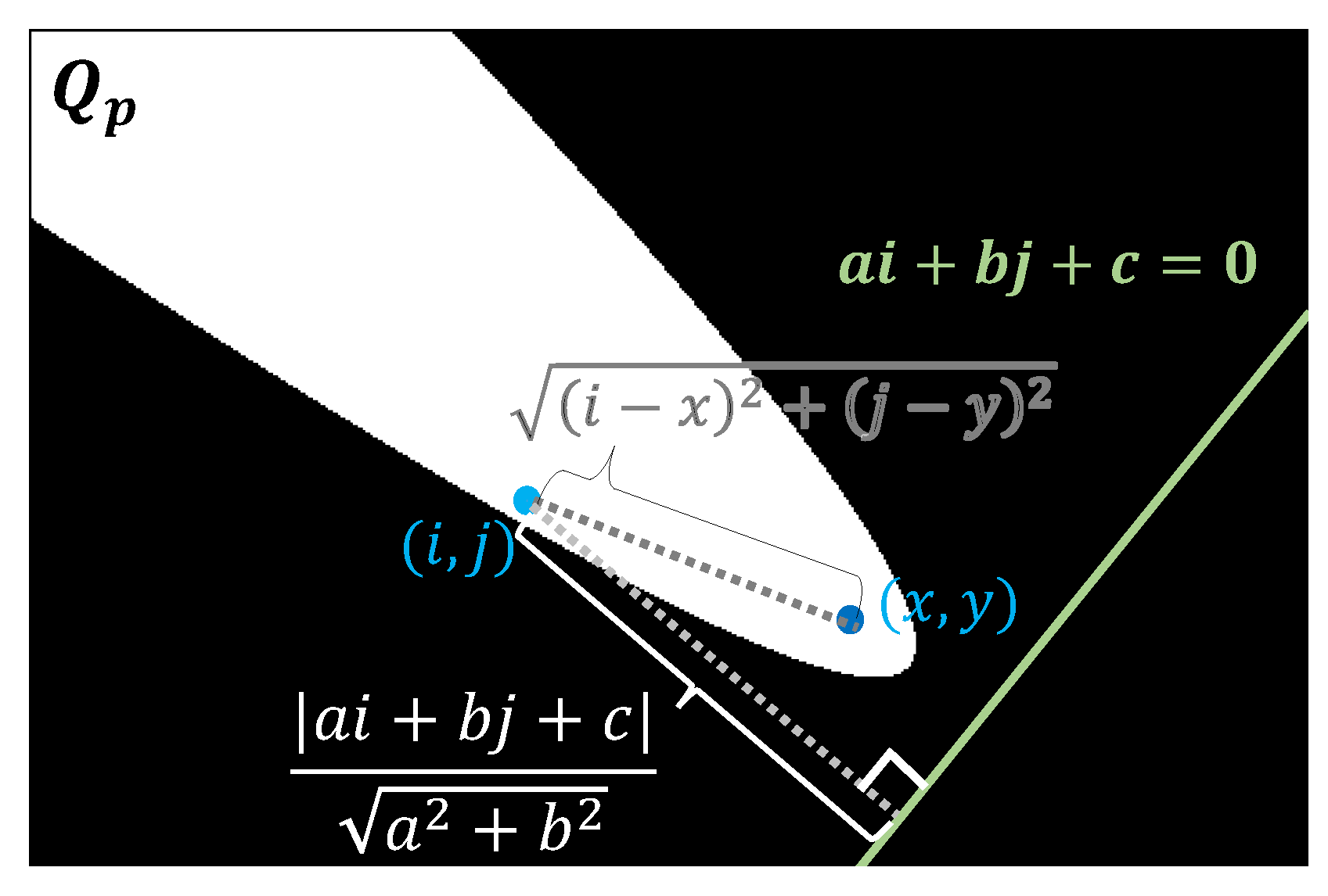
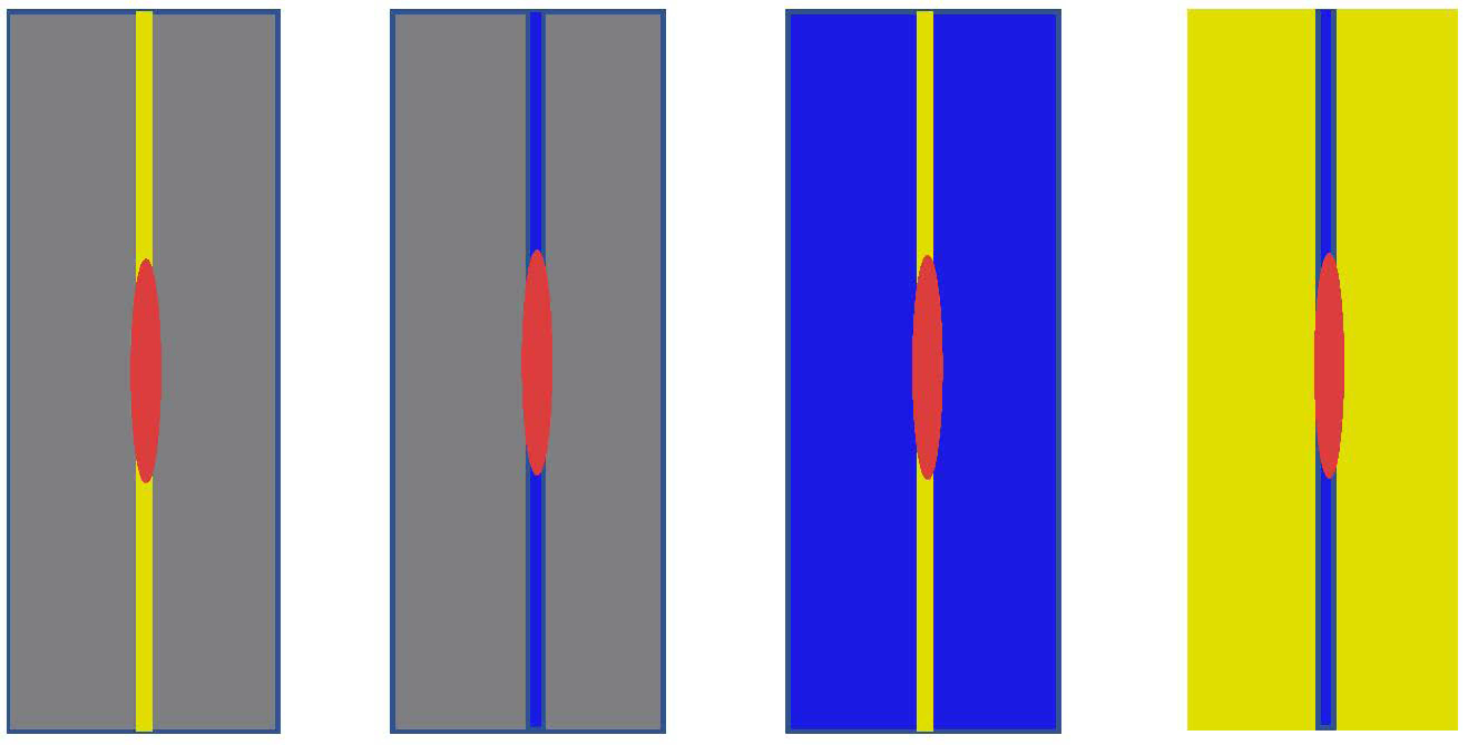
3.3.2. Directional Diffusion

The diffusion by GF or JBF can be realized by filtering multiple source points as input images or convoluting a kernel point by point. Since the number of sample points is tiny relative to the input image, the latter definition runs faster than the former methods. In the case of DTF and AMF, these kernels cannot be defined directly; thus, they can only be generated by convolving the sample points as an image. However, both are efficient filters that run in constant-time relative to the kernel radius.
Next, we introduce directional diffusion. The directionality can be created by cropping the region of PSF with a rotational quadratic function. The internal set in the rotational quadratic function Q p is defined by
Q p = ( i , j ) ( i x ) 2 + ( j y ) 2 a i + b j + c 2 a 2 + b 2 ,
where ( i , j ) S and p = ( x , y ) S are the s PSF pixel position and a sampling point, respectively. In this case, the sampling point is a focusing point, and the line, a i + b j + c = 0 , is a directrix of the quadratic function. A result of applying Equation (11) to a white image is shown in Figure 7. The white area in Figure 7 is the set of Q p .
Finally, directional light is generated based on any PSF by cropping the parabola function:
P p n = P p n p Q p 0 otherwise .
Since it is a cropping function, any PSF used in (7) is possible: GF, BF, or any other convolutional PSF.

3.4. Retinex-Based Image Relighting

The output image J : S R consists of luminance and reflectance factors, and our retouching aims to change the image’s illumination; thus, we change the luminance L by a luminance remapping function M while keeping the reflectance R :
J = M ( L ) R , where M ( L ) = ( l + k F ) L .
The function M is based on the illuminated map F computed in the previous section. Equation (13) shows that the lighting map boosts the luminance F by multiplying a constant scalar factor k, linearly darkening the factor l 1 . When l = 0.5 , the default lightness is half. Plugging in the Retinex relation of Equation (1), we can simplify Equation (13) as follows:
J = ( l + k F ) L R = ( l + k F ) L f L = ( l + k F ) f .
In our condition, we assume that illumination signals change linear properties; thus, the illumination component L can be removed in the final representation since the illumination components of L are canceled, i.e., there is no illumination L and reflectance R in (14). If we change L using a non-linear function, e.g., Gamma correction, the luminance component is required to recover the final image J . In this case, we should consider the color distortion problem [4], as in low-light enhancement.
The parameters l and k have essential roles in Retinex theory. Based on Retinex theory, human perception is affected by the surrounding colors. For example, in Figure 8, the two left gray backgrounds and the two right blue backgrounds, the RGB of the orange on the left side of each pair is ( 231 , 153 , 99 ) and that of the orange on the right side is ( 207 , 125 , 70 ) . In the images with blue backgrounds, the actual brightness of the oranges on the left and right sides is different, but they appear to be the same color. On the other hand, on the gray backgrounds, the oranges appear to have a greater difference in brightness than on the blue backgrounds, making it difficult to see the same color. This effect plays an important role in Retinex-based image processing. The dynamic range of an output image on display is generally 0 to 255. Therefore, when light is added to the original image, for example, the green light may not appear green due to the upper limit of the dynamic range (Figure 9a,d). To eliminate this effect, we reduce the brightness of the surroundings to make them appear relatively brighter (Figure 9b,c,e). Figure 9b,e are darkened in the RGB color space. Figure 9b,e are darkened in the Lab color space. In this paper, we used the second method and controlled for it using l of Equation (14).
Our human senses are also affected by the colors of our surroundings. In other words, the surrounding bright colors affect the new color to be added. Figure 10 shows the simulated example of the effect. The target pink colors have the same RGB values; however, these are affected by surrounding colors, and thus, these have different values. For example, it looks orange when the target color on the right-most side is enclosed by yellow. Therefore, we control the color using the Lab color space.
Equation (14) is changed to handle the Lab color space:
J = ( 1 + k F ) Lab 2 RGB ( l f L a b ) ,
where f L a b is the f in the Lab color space, and Lab 2 RGB ( · ) is a function that reconverts the Lab color space to RGB color space. Note that the vector l = { l l , l a , l b } has a similar role as a scalar l in Equation (14). The vector is extended to control the Lab values separately. If the elements in l for a and b channels components in the Lab color space are small, the output image has low color saturation.
Figure 11 shows the effect of surrounding colors by changing the parameter l . When l a and l b have low values, the color saturation values of the surrounding color are low. While these have high values, the color saturation values are high. The newly added light will be affected by the surrounding color situation and will change; thus, the user needs to make the desired changes.

4. Experimental Results

We performed two experiments: a comparison of the sampling methods and a visual comparison of the relighting results. We used eight images for the experiments, as shown in Figure 12.

4.1. Sampling Method Comparison

We verified the effectiveness of the sampling methods. In this experiment, we measured the probability that the sampled point was in the lighted object. We performed the following steps to determine whether light source points are inside or outside the lighted objects. First, we converted the input image into the 8-bit grayscale image and extracted its reflectance with thresholding by a threshold value T, where T = 50 for excluding outliers such as holes, windows, and the sky. For each image, Gaussian noises (mean: 0, standard deviation: 5) were added, and we performed the experiment 100 times to generate randomness. We experimentally compared state-of-the-art Retinex algorithms (URetinex-Net [59] and LR3M [6]) and saliency map algorithms (OpenCV implementation and SaliencyELD [60]) as sampling distributions for dithering. In addition, we handle random sampling as a baseline. The random sampling results can be directly computed as a percentage of the number of thresholds satisfied. Otherwise, it finds the percentage of dithering points below the threshold value.
Table 1 shows the mean ratio. Random sampling tends to have outside points since the sampling is not affected by luminance. The latest Retinex algorithm not only selects bright areas well, but samples the dark areas well too because these algorithms are designed to enhance dark images; they are thus unsuitable for this application. On the other hand, the proposed method can suppress light outside the object by using min-filtering and JBF. The latest saliency algorithms work better than the competitive Retinex algorithms. The proposed method works best because the algorithm is designed for the proposed new application of night image relighting.

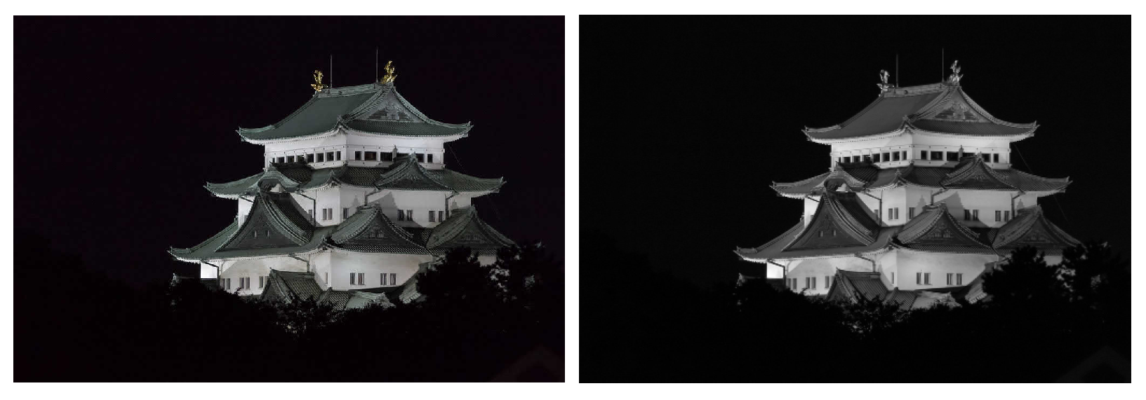
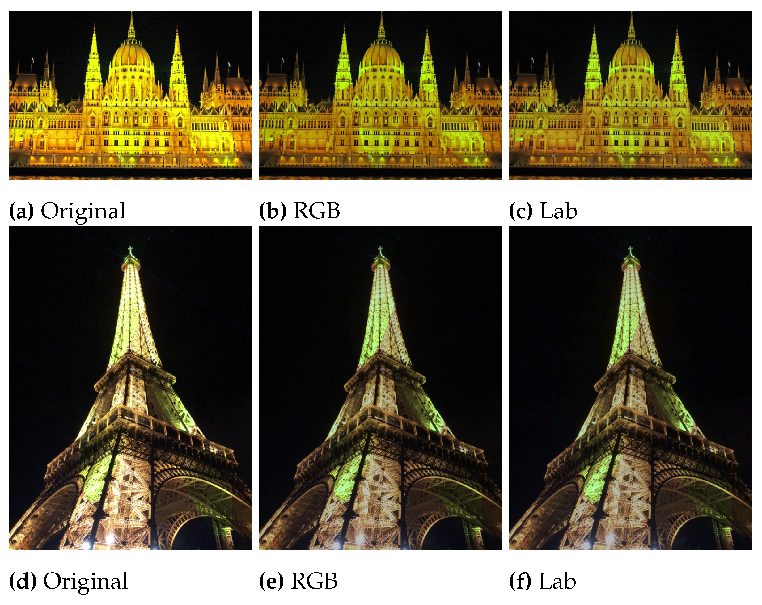
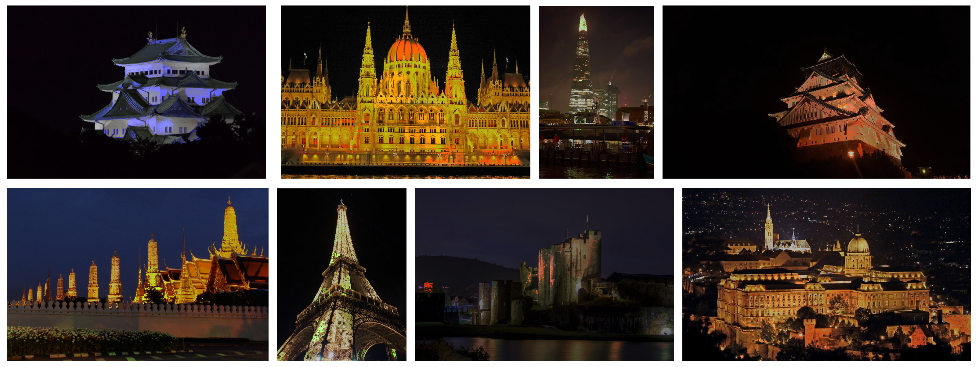
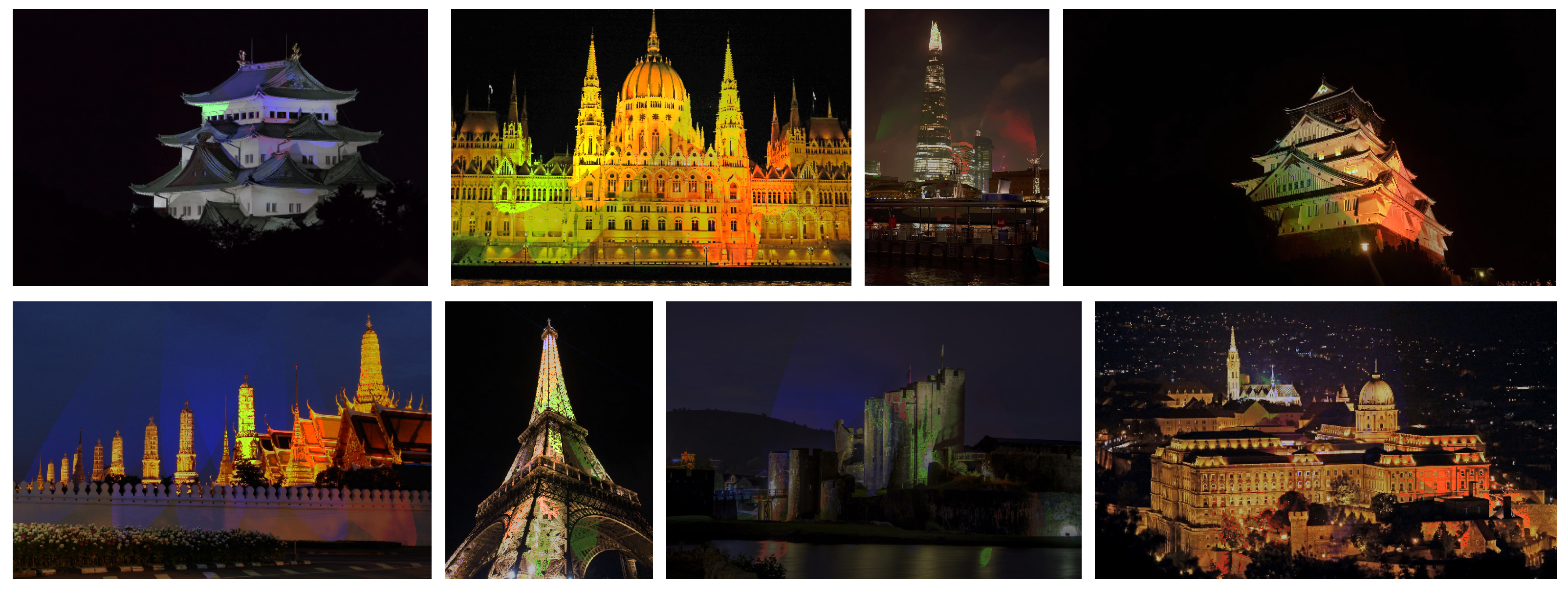
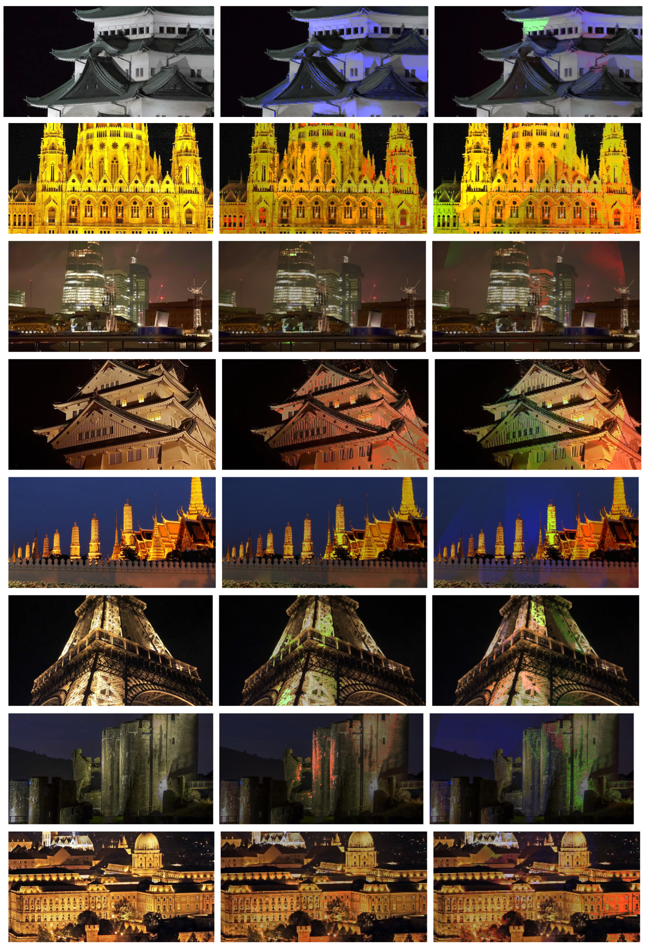
4.2. Visual Comparison

In this section, we visually compare each method. First, we compared with a light that spreads omnidirectionally from a point source using four different filters: GF (Figure 13a), JBF (Figure 13b), DTF (Figure 13c), and AMF (Figure 13d). Each filter diffuses a light source, and JBF, DTF, and AMF use the input image as a guided image. GF diffused regardless of the object boundary and even illuminated dark areas (Figure 13e). On the other hand, edge-preserving filters had weights depending on the difference in the guide image to prevent color leaking between different objects. JBF is characterized as being able to spread object awareness over a wide area (Figure 13f). In addition, JBF can also be spread out similar to GF regardless of the object by making the range smoothing parameter σ r infinitely large. DTF and AMF are characterized to illuminate the light more locally (Figure 13b,g,h). Each edge-preserving filter, JBF, DTF, and AMF, suppresses subnormal numbers to accelerate their filtering speeds [61], and the slower method of JBF is also accelerated by vectorization [62].
Next, we compared the directional light generation algorithms with the PSFs of GF and JBF using the SSR reflectance and the proposed reflectance. Figure 14 shows the diffusing lights and the rendering results. With the SSR reflectance, the sampling points tend to be located outside of the subject; thus, light leaks out of the object. The JBF PSF can reduce leakage to some extent, but it is challenging when completely outside the points. With the proposed reflectance, the sampling points concentrate on the subject, and the JBF PSF further concentrates the light within the subject. The other rendering results by the proposed reflectance, and JBF with changing color are shown in Figure 15 (omnidirectional) and Figure 16 (directional). The expanded images of Figure 15 and Figure 16 are shown in Figure 17.

5. Conclusions

In this paper, we proposed a relighting method for night photography in the form of a new Retinex-based application. We proposed a method for selecting points of relighting and synthesizing them using human perceptual characteristics according to Retinex theory. In addition, multiple diffusion methods were proposed to enable a variety of representations, such as omnidirectional diffusion and directional diffusion with and without various edge-preserving properties.

Author Contributions

Conceptualization, N.F.; methodology, N.F. and S.O.; software, N.F. and S.O.; validation, S.O.; formal analysis, N.F. and S.O.; investigation, N.F. and S.O.; resources, N.F. and S.O.; data curation, S.O.; writing—original draft preparation, S.O.; writing—review and editing, N.F.; visualization, N.F. and S.O.; supervision, N.F.; project administration, N.F.; funding acquisition, N.F. All authors have read and agreed to the published version of the manuscript.

Funding

Norishige Fukushima was supported by JSPS KAKENHI (21H03465).

Institutional Review Board Statement

Not applicable.

Informed Consent Statement

Not applicable.

Data Availability Statement

Our code, dataset, and additional results are available at https://norishigefukushima.github.io/RelightingUpNightPhotography/ accessed on 25 January 2023.

Acknowledgments

We thank Aiko Iwase (Tajimi Iwase Eye Clinic) for her support.

Conflicts of Interest

The authors declare no conflict of interest.

Abbreviations

The following abbreviations are used in this manuscript:
HSVhuman visual system
SSRsingle-scale Retinex
MSRmulti-scale Retinex
DCTdiscrete cosine transform
FFTfast Fourier transform
BFbilateral filtering
JBFjoint bilateral filtering
PSFpoint spread function
GFGaussian filtering
DTFdomain transform filtering
AMFadaptive manifolds filtering

Appendix A. Symbols Table

a, b, cparameters of quadratic function
A set of light source samples
Bvalue of maximum intensity (brightness)
dnumber of dimensions for color signals
C vector of user-determined light color
Dnumber of dimensions
D set of dithering points
f input image ( f p , f q : intensity vectors of pixel positions p and q )
f o derived function of f at o
F illuminating color map
gGaussian convolution operator
hvariable of a histogram index in clipping linear function
i, jcoordinates of an arbitrary point in the quadratic function Q
tnumber of JBF iterations
J output image
kconstant scalar factor that enhances luminance
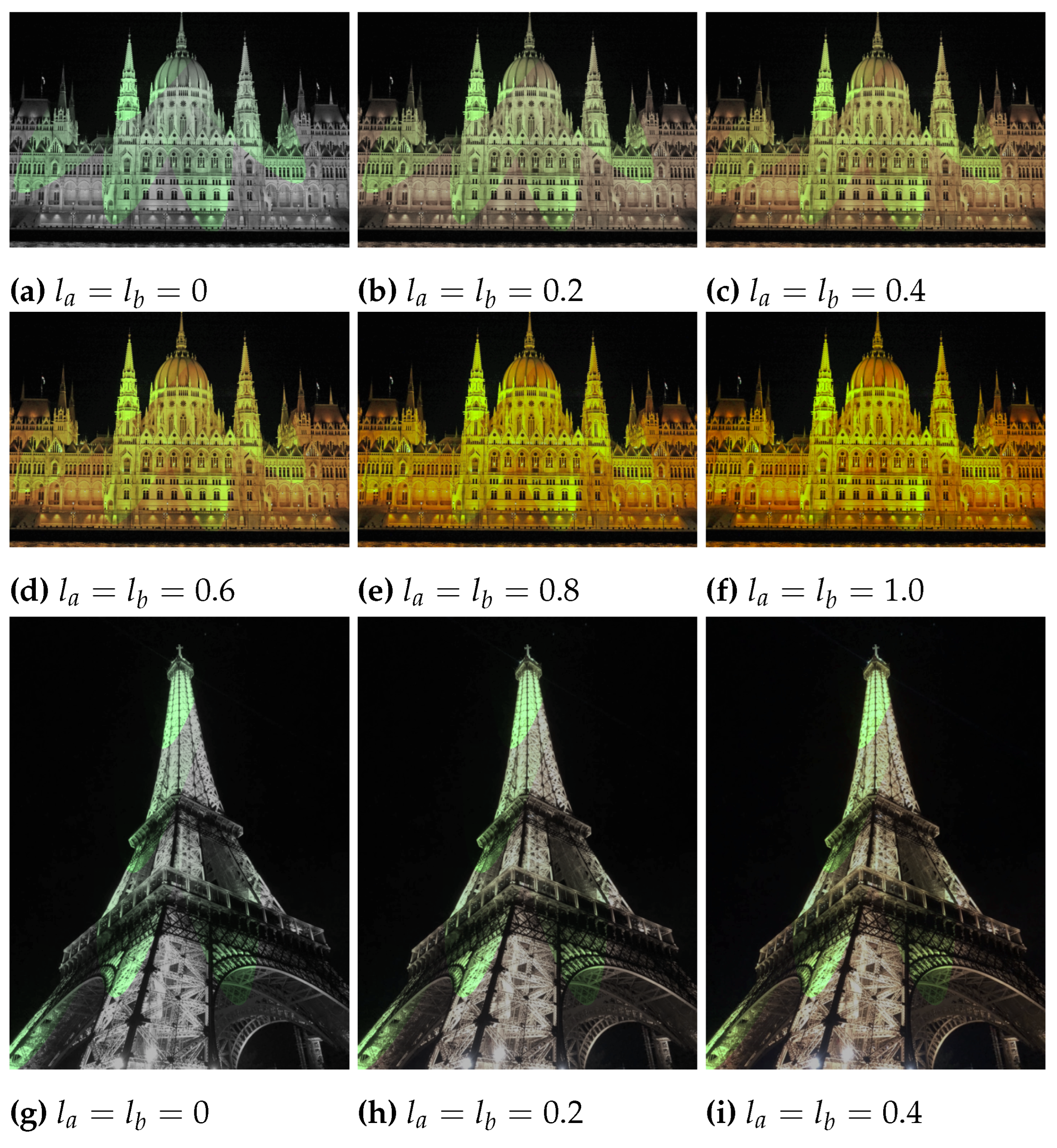
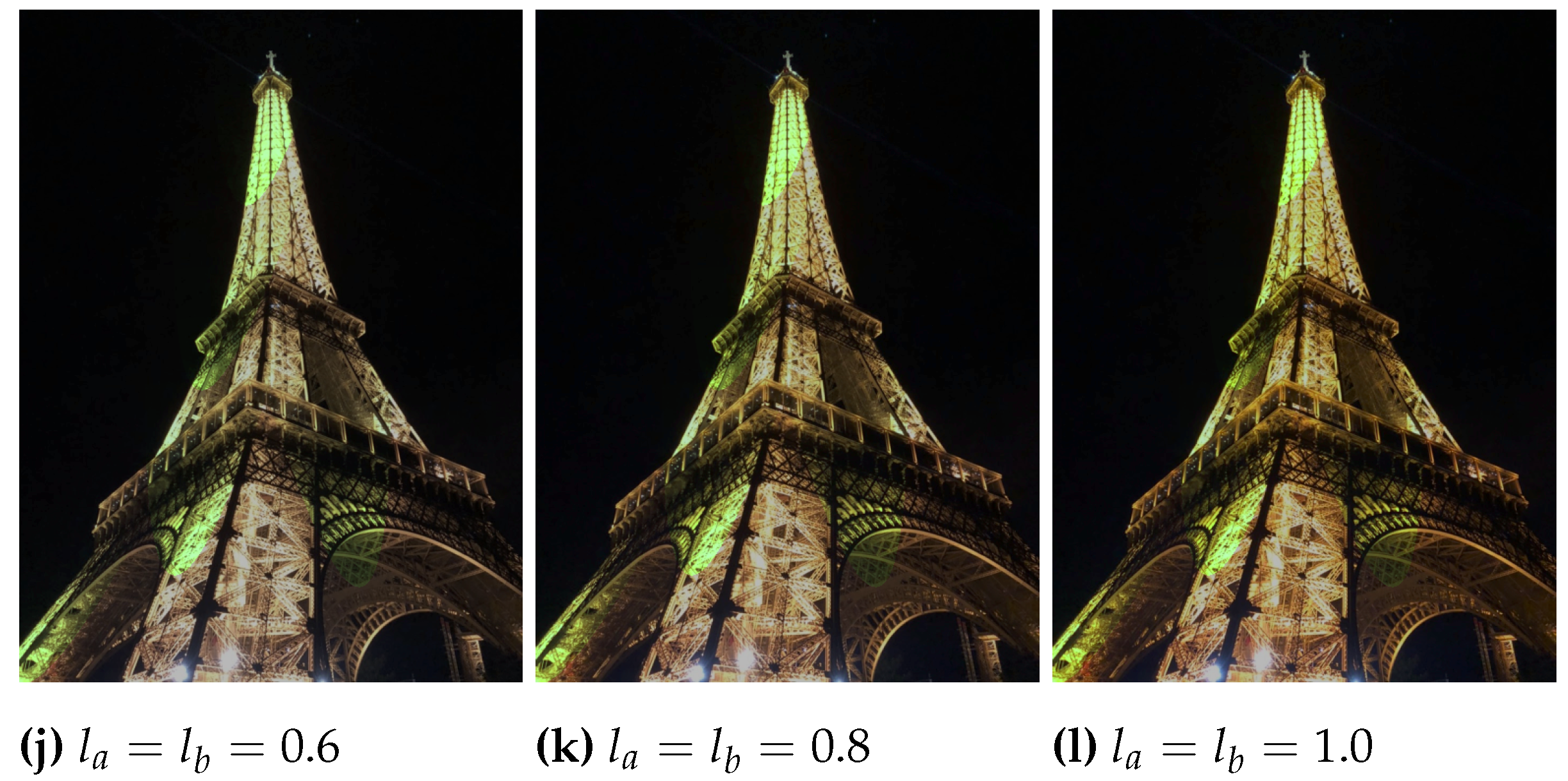
 F
l l , l a , l b linearly darkening factor in Lab color space
L illumination map
M ( ) luminance remapping function
nsubscript representing the index ( P n and C n )
Nnumber of samples ( N d : desired number of samples,
N l : number of target samples), N: number of image pixels
p , q pixel position
P n , P n PSF for n-th sampling point and its cropping version
Qset of clipped quadratic function
r l minimum distance between light source points
rsubscript of a smoothing parameter σ r
R reflectance map ( R p : intensity vectors of pixel positions p )
R set of real numbers
R range domain
ssubscript of a smoothing parameter σ s
S spatial domain
S saliency map ( S t )
titerating subscript (e.g., S t )
Tthreshold value used in our experiment
U ( ) clipping linear function ( R ( x , s ) )
vvariable of saturation-clipping linear function ( R ( x , s ) )
w s , w r weight function for edge-preserving smoothing filtering
x , y coordinates of light source for defining Q
γ amplify parameter for r l , e.g., γ r l
σ , σ s , σ r smoothing parameters
Ω set of neighboring pixels of a pixel (e.g., Ω p )

References

  1. Land, E.H. The retinex. Am. Sci. 1964, 52, 247–264. [Google Scholar]
  2. Land, E.H. The retinex theory of color vision. Sci. Am. 1977, 237, 108–129. [Google Scholar] [CrossRef]
  3. Land, E.H. An alternative technique for the computation of the designator in the retinex theory of color vision. Proc. Natl. Acad. Sci. USA 1986, 83, 3078–3080. [Google Scholar] [CrossRef] [Green Version]
  4. Rahman, Z.U.; Jobson, D.J.; Woodell, G.A. Retinex processing for automatic image enhancement. J. Electron. Imaging 2004, 13, 100–110. [Google Scholar] [CrossRef]
  5. Guo, X.; Li, Y.; Ling, H. LIME: Low-light image enhancement via illumination map estimation. IEEE Trans. Image Process. 2016, 26, 982–993. [Google Scholar] [CrossRef] [PubMed]
  6. Ren, X.; Yang, W.; Cheng, W.H.; Liu, J. LR3M: Robust low-light enhancement via low-rank regularized retinex model. IEEE Trans. Image Process. 2020, 29, 5862–5876. [Google Scholar] [CrossRef]
  7. Xu, J.; Hou, Y.; Ren, D.; Liu, L.; Zhu, F.; Yu, M.; Wang, H.; Shao, L. Star: A structure and texture aware retinex model. IEEE Trans. Image Process. 2020, 29, 5022–5037. [Google Scholar] [CrossRef] [Green Version]
  8. Kong, X.Y.; Liu, L.; Qian, Y.S. Low-light image enhancement via poisson noise aware retinex model. IEEE Signal Process. Lett. 2021, 28, 1540–1544. [Google Scholar] [CrossRef]
  9. Tang, H.; Zhu, H.; Tao, H.; Xie, C. An Improved Algorithm for Low-Light Image Enhancement Based on RetinexNet. Appl. Sci. 2022, 12, 7268. [Google Scholar] [CrossRef]
  10. Pan, X.; Li, C.; Pan, Z.; Yan, J.; Tang, S.; Yin, X. Low-Light Image Enhancement Method Based on Retinex Theory by Improving Illumination Map. Appl. Sci. 2022, 12, 5257. [Google Scholar] [CrossRef]
  11. Meylan, L.; Susstrunk, S. High dynamic range image rendering with a retinex-based adaptive filter. IEEE Trans. Image Process. 2006, 15, 2820–2830. [Google Scholar] [CrossRef] [PubMed]
  12. Parthasarathy, S.; Sankaran, P. A RETINEX based haze removal method. In Proceedings of the IEEE International Conference on Industrial and Information Systems (ICIIS), Chennai, India, 6–9 August 2012. [Google Scholar] [CrossRef]
  13. Galdran, A.; Alvarez-Gila, A.; Bria, A.; Vazquez-Corral, J.; Bertalmío, M. On the duality between retinex and image dehazing. In Proceedings of the IEEE Conference on Computer Vision and Pattern Recognition (CVPR), Salt Lake City, UT, USA, 18–23 June 2018; pp. 8212–8221. [Google Scholar] [CrossRef] [Green Version]
  14. Zhuang, P.; Li, C.; Wu, J. Bayesian retinex underwater image enhancement. Eng. Appl. Artif. Intell. 2021, 101, 104171. [Google Scholar] [CrossRef]
  15. Finlayson, G.D.; Hordley, S.D.; Drew, M.S. Removing shadows from images using retinex. In Proceedings of the Color and Imaging Conference, Scottsdale, AZ, USA, 12–15 November 2002; pp. 73–79. [Google Scholar]
  16. Rizzi, A.; Gatta, C.; Marini, D. From retinex to automatic color equalization: Issues in developing a new algorithm for unsupervised color equalization. J. Electron. Imaging 2004, 13, 75–84. [Google Scholar] [CrossRef] [Green Version]
  17. Okuhata, H.; Nakamura, H.; Hara, S.; Tsutsui, H.; Onoye, T. Application of the real-time Retinex image enhancement for endoscopic images. In Proceedings of the Annual International Conference of the IEEE Engineering in Medicine and Biology Society (EMBC), Osaka, Japan, 3–7 July 2013; pp. 3407–3410. [Google Scholar] [CrossRef]
  18. Almalki, Y.E.; Jandan, N.A.; Soomro, T.A.; Ali, A.; Kumar, P.; Irfan, M.; Keerio, M.U.; Rahman, S.; Alqahtani, A.; Alqhtani, S.M.; et al. Enhancement of Medical Images through an Iterative McCann Retinex Algorithm: A Case of Detecting Brain Tumor and Retinal Vessel Segmentation. Appl. Sci. 2022, 12, 8243. [Google Scholar] [CrossRef]
  19. Park, Y.K.; Park, S.L.; Kim, J.K. Retinex method based on adaptive smoothing for illumination invariant face recognition. Signal Process. 2008, 88, 1929–1945. [Google Scholar] [CrossRef]
  20. Park, S.; Yu, S.; Moon, B.; Ko, S.; Paik, J. Low-light image enhancement using variational optimization-based retinex model. IEEE Trans. Consum. Electron. 2017, 63, 178–184. [Google Scholar] [CrossRef]
  21. Jobson, D.J.; Rahman, Z.u.; Woodell, G.A. Properties and performance of a center/surround retinex. IEEE Trans. Image Process. 1997, 6, 451–462. [Google Scholar] [CrossRef]
  22. Eisemann, E.; Durand, F. Flash Photography Enhancement via Intrinsic Relighting. ACM Trans. Graph. 2004, 673–678. [Google Scholar] [CrossRef]
  23. Petschnigg, G.; Agrawala, M.; Hoppe, H.; Szeliski, R.; Cohen, M.; Toyama, K. Digital Photography with Flash and No-flash Image Pairs. ACM Trans. Graph. 2004, 23, 664–672. [Google Scholar] [CrossRef] [Green Version]
  24. Chen, S.; Haralick, R.M. Recursive erosion, dilation, opening, and closing transforms. IEEE Trans. Image Process. 1995, 4, 335–345. [Google Scholar] [CrossRef]
  25. Otsuka, T.; Fukushima, N.; Maeda, Y.; Sugimoto, K.; Kamata, S. Optimization of Sliding-DCT based Gaussian Filtering for Hardware Accelerator. In Proceedings of the International Conference on Visual Communications and Image Processing (VCIP), Macau, China, 1–4 December 2020. [Google Scholar] [CrossRef]
  26. Sumiya, Y.; Fukushima, N.; Sugimoto, K.; Kamata, S. Extending Compressive Bilateral Filtering for Arbitrary Range Kernel. In Proceedings of the IEEE International Conference on Image Processing (ICIP), Abu Dhabi, United Arab, 25–28 October 2020. [Google Scholar] [CrossRef]
  27. He, K.; Sun, J.; Tang, X. Single image haze removal using dark channel prior. IEEE Trans. Pattern Anal. Mach. Intell. 2010, 33, 2341–2353. [Google Scholar] [CrossRef] [PubMed]
  28. He, K.; Shun, J.; Tang, X. Guided Image Filtering. In Proceedings of the European Conference on Computer Vision (ECCV), Heraklion, Crete, Greece, 5–11 September 2010. [Google Scholar] [CrossRef]
  29. Fukushima, N.; Sugimoto, K.; Kamata, S. Guided Image Filtering with Arbitrary Window Function. In Proceedings of the IEEE International Conference on Acoustics, Speech and Signal Processing, Calgary, AB, Canada, 15–20 April 2018. [Google Scholar] [CrossRef]
  30. Cook, R.L. Stochastic sampling in computer graphics. ACM Trans. Graph. (TOG) 1986, 5, 51–72. [Google Scholar] [CrossRef]
  31. Zosso, D.; Tran, G.; Osher, S.J. Non-Local Retinex—A Unifying Framework and Beyond. SIAM J. Imaging Sci. 2015, 8, 787–826. [Google Scholar] [CrossRef]
  32. McCann, J.J. Retinex at 50: Color theory and spatial algorithms, a review. J. Electron. Imaging 2017, 26, 031204. [Google Scholar] [CrossRef]
  33. Horn, B.K. Determining lightness from an image. Comput. Graph. Image Process. 1974, 3, 277–299. [Google Scholar] [CrossRef]
  34. Morel, J.M.; Petro, A.B.; Sbert, C. A PDE formalization of Retinex theory. IEEE Trans. Image Process. 2010, 19, 2825–2837. [Google Scholar] [CrossRef]
  35. Funt, B.V.; Ciurea, F.; McCann, J.J. Retinex in MATLABTM. J. Electron. Imaging 2004, 13, 48–57. [Google Scholar] [CrossRef]
  36. Rahman, Z.u.; Jobson, D.J.; Woodell, G.A. Multi-scale retinex for color image enhancement. In Proceedings of the IEEE international conference on image processing (ICIP), Lausanne, Switzerland, 19 September 1996; Volume 3, pp. 1003–1006. [Google Scholar] [CrossRef]
  37. Jobson, D.J.; Rahman, Z.; Wooden, G.A. A multiscale retinex for bridging the gap between color images and the human observation of scenes. IEEE Trans. Image Process. 1997, 6, 965–976. [Google Scholar] [CrossRef] [PubMed] [Green Version]
  38. Kimmel, R.; Elad, M.; Shaked, D.; Keshet, R.; Sobel, I. A variational framework for retinex. Int. J. Comput. Vis. 2003, 52, 7–23. [Google Scholar] [CrossRef]
  39. Elad, M. Retinex by two bilateral filters. In Proceedings of the International Conference on Scale-Space Theories in Computer Vision, Hofgeismar, Germany, 7–9 April 2005; pp. 217–229. [Google Scholar] [CrossRef]
  40. Wei, C.; Wang, W.; Yang, W.; Liu, J. Deep Retinex Decomposition for Low-Light Enhancement. In Proceedings of the British Machine Vision Conference (BMVC), Newcastle, UK, 3–6 September 2018. [Google Scholar]
  41. Li, P.; Tian, J.; Tang, Y.; Wang, G.; Wu, C. Deep retinex network for single image dehazing. IEEE Trans. Image Process. 2020, 30, 1100–1115. [Google Scholar] [CrossRef] [PubMed]
  42. Grosse, R.; Johnson, M.; Adelson, E.; Freeman, W. Ground-truth dataset and baseline evaluations for intrinsic image algorithms. In Proceedings of the International Conference on Computer Vision (ICCV), Kyoto, Japan, 29 September–2 October 2009; pp. 2335–2342. [Google Scholar] [CrossRef]
  43. Gehler, P.; Rother, C.; Kiefel, M.; Zhang, L.; Scholkopf, B. Recovering intrinsic images with a global sparsity prior on reflectance. In Proceedings of the Neural Information Processing Systems (NIPS), Granada, Spain, 12–17 December 2011; pp. 765–773. [Google Scholar]
  44. Barron, J.; Malik, J. Color constancy, intrinsic images, and shape estimation. In Proceedings of the European Conference on Computer Vision (ECCV), Firenze, Italy, 7–13 October 2012; pp. 57–70. [Google Scholar] [CrossRef]
  45. Li, Y.; Brown, M. Single image layer separation using relative smoothness. In Proceedings of the Computer Vision and Pattern Recognition Conference (CVPR), Columbus, OH, USA, 23–28 June 2014; pp. 2752–2759. [Google Scholar] [CrossRef]
  46. Land, E.H.; McCann, J.J. Lightness and retinex theory. J. Opt. Soc. Am. 1971, 61, 1–11. [Google Scholar] [CrossRef]
  47. Ciurea, F.; Funt, B.V. Tuning retinex parameters. J. Electron. Imaging 2004, 13, 58–64. [Google Scholar] [CrossRef] [Green Version]
  48. Itti, L.; Koch, C.; Niebur, E. A model of saliency-based visual attention for rapid scene analysis. IEEE Trans. Pattern Anal. Mach. Intell. 1998, 20, 1254–1259. [Google Scholar] [CrossRef] [Green Version]
  49. Sugimoto, K.; Kamata, S. Efficient constant-time Gaussian filtering with sliding DCT/DST-5 and dual-domain error minimization. ITE Trans. Media Technol. Appl. 2015, 3, 12–21. [Google Scholar] [CrossRef] [Green Version]
  50. Sugimoto, K.; Kyochi, S.; Kamata, S. Universal approach for DCT-based constant-time Gaussian filter with moment preservation. In Proceedings of the IEEE International Conference on Acoustics, Speech and Signal Processing (ICASSP), Calgary, AB, Canada, 15–20 April 2018. [Google Scholar] [CrossRef]
  51. Fukushima, N.; Maeda, Y.; Kawasaki, Y.; Nakamura, M.; Tsumura, T.; Sugimoto, K.; Kamata, S. Efficient Computational Scheduling of Box and Gaussian FIR Filtering for CPU Microarchitecture. In Proceedings of the Asia-Pacific Signal and Information Processing Association Annual Summit and Conference (APSIPA ASC), Honolulu, HI, USA, 12–15 November 2018. [Google Scholar] [CrossRef]
  52. Tomasi, C.; Manduchi, R. Bilateral Filtering for Gray and Color Images. In Proceedings of the IEEE International Conference on Computer Vision (ICCV), Bombay, India, 7 January 1998. [Google Scholar] [CrossRef]
  53. Sugimoto, K.; Fukushima, N.; Kamata, S. 200 FPS Constant-time Bilateral Filter Using SVD and Tiling Strategy. In Proceedings of the IEEE International Conference on Image Processing (ICIP), Taipei, Taiwan, 22–25 September 2019. [Google Scholar] [CrossRef]
  54. Ulichney, R.A. Dithering with blue noise. Proc. IEEE 1988, 76, 56–79. [Google Scholar] [CrossRef]
  55. Mitsa, T.; Parker, K. Digital halftoning using a blue noise mask. In Proceedings of the International Conference on Acoustics, Speech, and Signal Processing (ICASSP), Toronto, ON, Canada, 14–17 April 1991. [Google Scholar] [CrossRef]
  56. Lou, L.; Nguyen, P.; Lawrence, J.; Barnes, C. Image Perforation: Automatically Accelerating Image Pipelines by Intelligently Skipping Samples. ACM Trans. Graph. 2016, 35, 1–14. [Google Scholar] [CrossRef]
  57. Gastal, E.S.L.; Oliveira, M.M. Domain Transform for Edge-Aware Image and Video Processing. ACM Trans. Graph. 2011, 30, 1–12. [Google Scholar] [CrossRef]
  58. Gastal, E.S.L.; Oliveira, M.M. Adaptive Manifolds for Real-Time High-Dimensional Filtering. ACM Trans. Graph. 2012, 31, 1–13. [Google Scholar] [CrossRef]
  59. Wu, W.; Weng, J.; Zhang, P.; Wang, X.; Yang, W.; Jiang, J. URetinex-Net: Retinex-Based Deep Unfolding Network for Low-Light Image Enhancement. In Proceedings of the Proceedings of the IEEE/CVF Conference on Computer Vision and Pattern Recognition (CVPR), New Orleans, LA, USA, 18–24 June 2022; pp. 5901–5910. [Google Scholar] [CrossRef]
  60. Gayoung, L.; Yu-Wing, T.; Junmo, K. Deep Saliency with Encoded Low level Distance Map and High Level Features. In Proceedings of the IEEE Conference on Computer Vision and Pattern Recognition (CVPR), Las Vegas, NV, USA, 27–30 June 2016. [Google Scholar] [CrossRef] [Green Version]
  61. Maeda, Y.; Fukushima, N.; Matsuo, H. Effective Implementation of Edge-Preserving Filtering on CPU Microarchitectures. Appl. Sci. 2018, 8, 1985. [Google Scholar] [CrossRef] [Green Version]
  62. Maeda, Y.; Fukushima, N.; Matsuo, H. Taxonomy of Vectorization Patterns of Programming for FIR Image Filters Using Kernel Subsampling and New One. Appl. Sci. 2018, 8, 1235. [Google Scholar] [CrossRef]
Figure 2. Input color and its grayscale images.
Applsci 13 01719 g002
Figure 3. Luminance L and reflectance R for each method: L is shared for each method, and the output is normalized for visibility. The proposed reflectance is SSR+min-filter+JBF.
Applsci 13 01719 g003
Figure 4. Restored image with multiplying R and L . (a) R is Figure 3b, and the output is the same as Figure 2 grayscale. (b) R is Figure 3c and the output is not recovered.
Applsci 13 01719 g004
Figure 5. Examples of blue noise sampling from dithering samples.
Applsci 13 01719 g005
Figure 6. Flowchart of sampling light source from dithering points.
Applsci 13 01719 g006
Figure 7. Visualizing result of (11). The white area is the set Q p .
Applsci 13 01719 g007
Figure 8. Effect of surrounding luminance values and colors on the brightness of target color. A blue and gray background pair, with the orange RGB value on the left (231,153,99) and on the right (207,125,70), respectively.
Applsci 13 01719 g008
Figure 9. Appearance when illuminated with awareness of dynamic range. (a,d): The luminance value is added to the original image. (b,e): The luminance value is added after darkening the original image by reducing RGB values ( l = 0.75 ). (c,f): The luminance value is added to the RGB image that is converted to Lab color space ( l l = l a = l b = 0.75 ).
Applsci 13 01719 g009
Figure 10. Color constancy affected by surrounding colors. All centering objects have the same color value (pink), but their appearances differ.
Applsci 13 01719 g010
Figure 11. Parameter changing results in Lab color space (Fixed l l = 0.75 with respect to l a and l b ).
Applsci 13 01719 g011aApplsci 13 01719 g011b
Figure 12. Test images.
Applsci 13 01719 g012
Figure 13. Comparison of 4 omnidirectional diffusion methods. (Top) PSFs; (Bottom) the output image with diffusion.
Applsci 13 01719 g013
Figure 14. Directional diffusing with 5 points selected: (a,b,e,f) from SSR, (c,d,g,h) from the proposed.
Applsci 13 01719 g014
Figure 15. Rendering results with omnidirectional diffusion (JBF).
Applsci 13 01719 g015
Figure 16. Rendering results with directional diffusion (JBF).
Applsci 13 01719 g016
Figure 17. Expansion of output (left: test images, center: Rendering results with omnidirectional diffusion, right: rendering results with directional diffusion (JBF)).
Applsci 13 01719 g017
Table 1. Probability that the points are out of the object (8-bit luminance value threshold: 50). Probability of random sampling points is the percentage above or below the threshold. The other probabilities are the percentage of cases where the dithering points of the input image are above or below the threshold. The top score for each image is shown in boldface.
ImageabcdefghAve.
Random0.86090.71730.90840.88960.81630.85660.86370.76970.8353
URetinex-Net [59]0.51590.43220.83070.53180.51790.61670.65960.38890.5617
LR3M [6]0.75390.4880.88460.84820.63640.80770.81140.59410.7280
Saliency (OpenCV)0.38310.47900.59800.29760.54830.51080.49660.59930.4891
SaliencyELD [60]0.42300.28320.43010.19450.31010.48580.30740.32160.3445
Proposed0.16180.32750.37270.13640.24940.21590.25560.28420.2504
Disclaimer/Publisher’s Note: The statements, opinions and data contained in all publications are solely those of the individual author(s) and contributor(s) and not of MDPI and/or the editor(s). MDPI and/or the editor(s) disclaim responsibility for any injury to people or property resulting from any ideas, methods, instructions or products referred to in the content.

