
A Novel Interval Iterative Multi-Thresholding Algorithm Based on Hybrid Spatial Filter and Region Growing for Medical Brain MR Images

Abstract
1. Introduction
- (1)
- A hybrid spatial filter is proposed to achieve image multi-scale decomposition which denoising while preserving more details. The proposed filter makes full use of the spatial information in the original image. It can improve the accuracy of image segmentation and make the algorithm more powerful and robust.
- (2)
- We proposed an interval iterative Otsu method based on region growing (RGIIM). It quickly obtains the growth threshold through the region growing method (RGM) and uses the idea of interval iteration to optimize the thresholds. This method achieves satisfactory segmentation results with minimal time cost.
- (3)
- A weighted strategy is used to fuse the segmentation result of the original image and its hybrid layers to make the final segmentation result more accurate.
2. Interval Iterative Otsu Method Based on Region Growing
2.1. Otsu Method
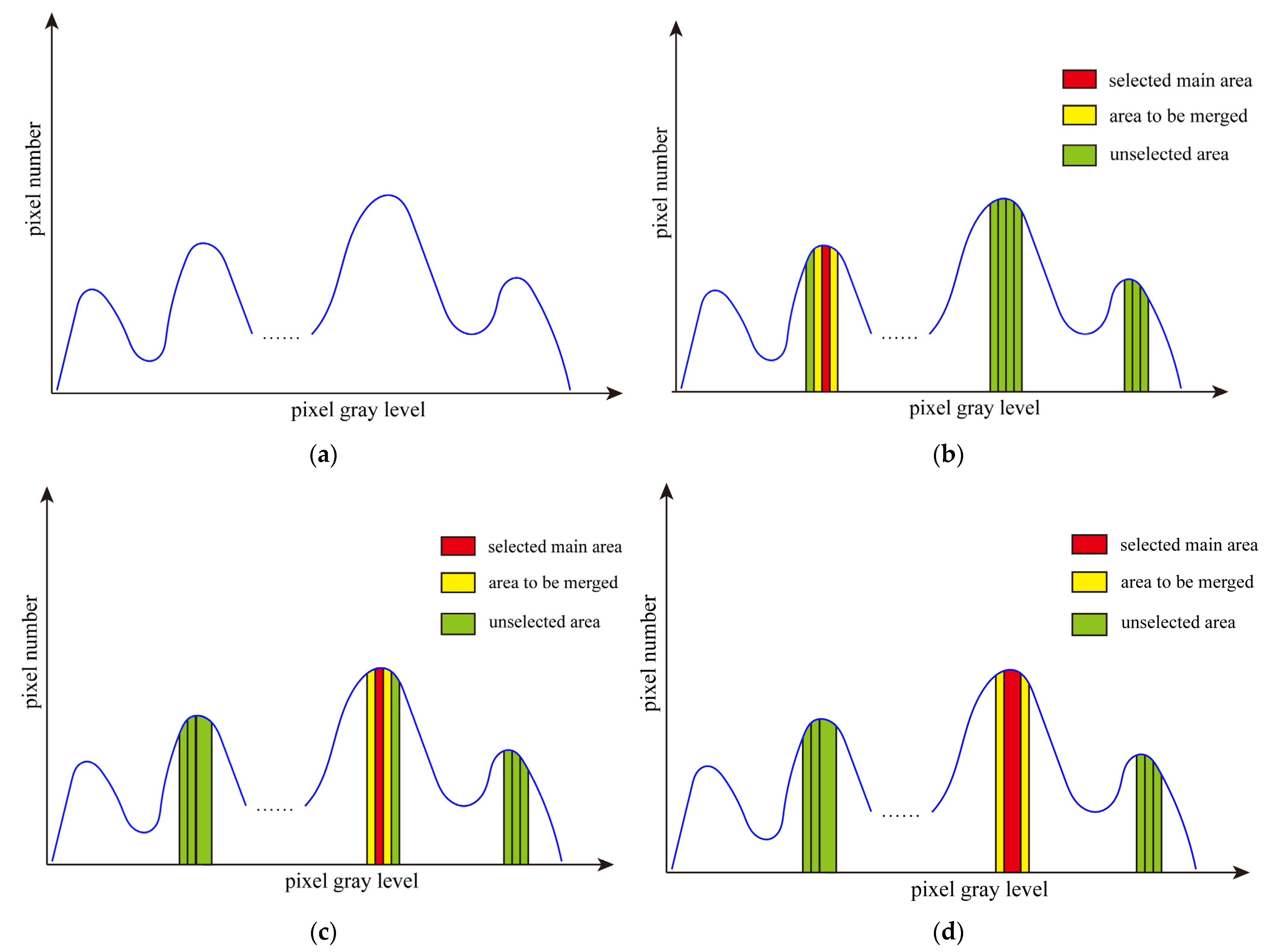
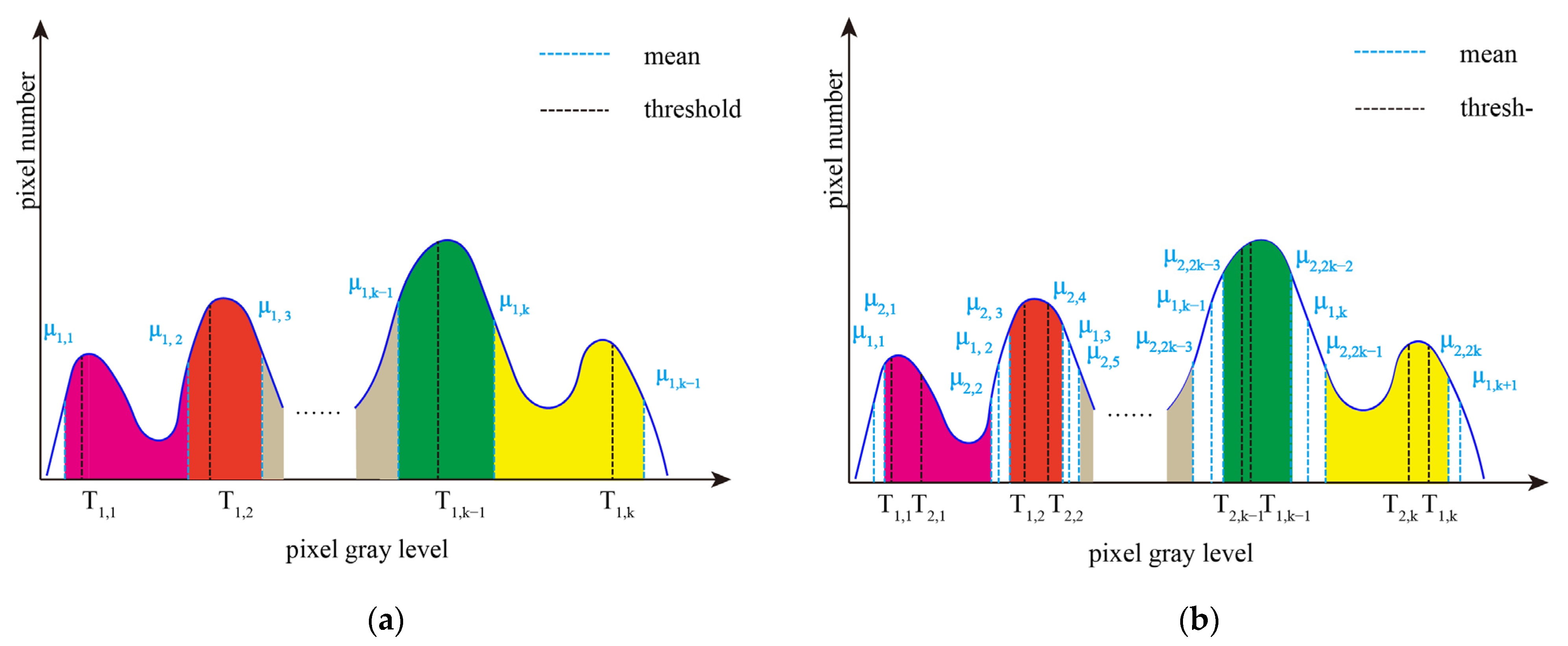
2.2. Interval Iterative Otsu Method Based on Region Growing
2.2.1. The First Stage
2.2.2. The Final Stage
3. The Proposed Algorithm
3.1. The Framework
- (1)
- The original image is processed with the proposed hybrid spatial filter to obtain the hybrid layer.
- (2)
- The proposed RGIIM is executed on the original image and the hybrid layer separately to obtain different sets of segmentation thresholds.
- (3)
- The weighted strategy is performed on the segmentation thresholds to obtained the optimized segmentation thresholds.
3.2. Hybrid Spatial Filter
3.3. Weighted Strategy
4. Experimental Results and Analysis
4.1. Experimental Protocols
4.2. Evaluation Measure
4.3. Comparison between the Proposed Method and Other Methods
4.4. Ablation Experiment
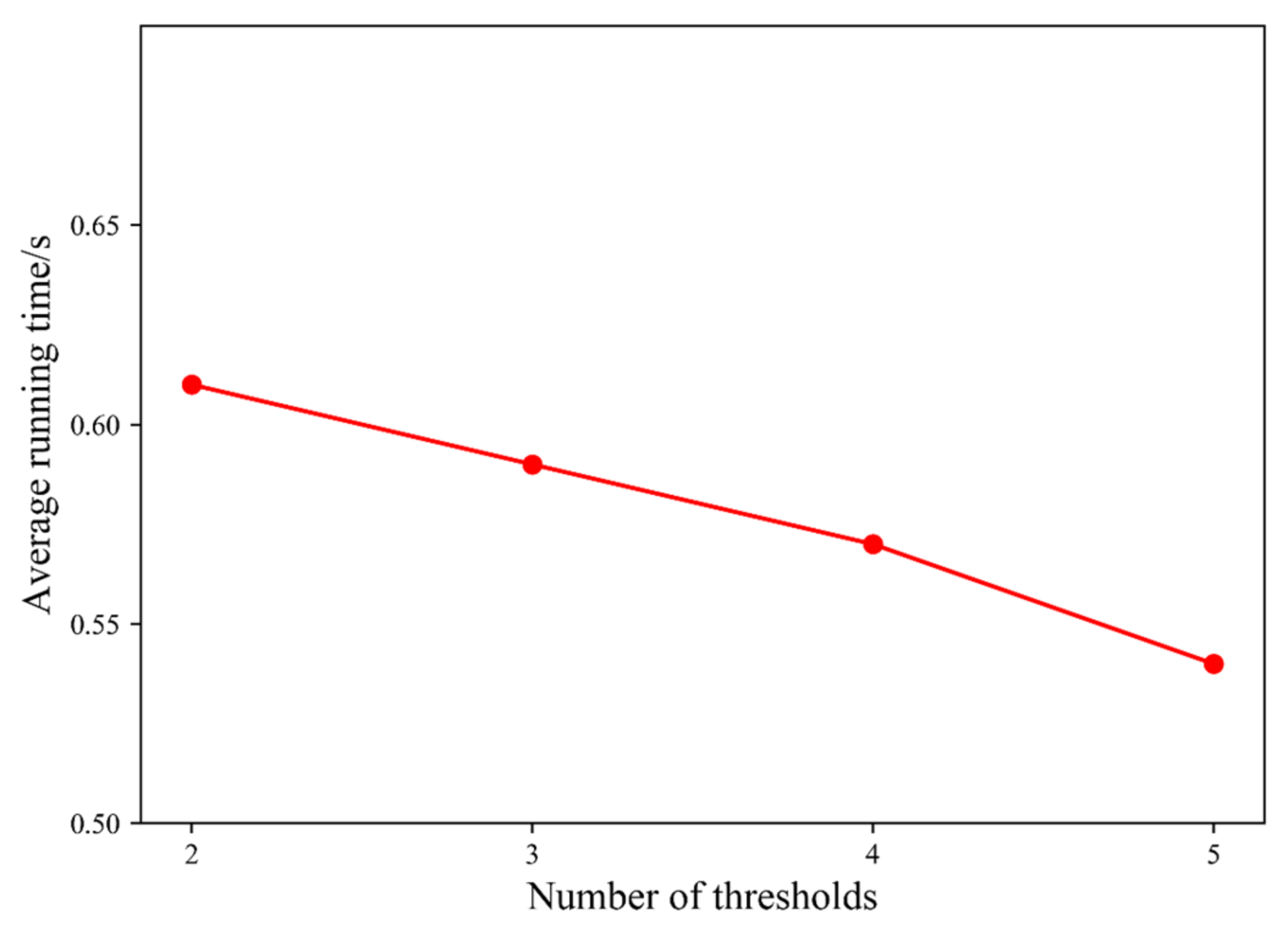
4.5. Time Complexity Analysis
4.5.1. Proposed Method Time Complexity Analysis
4.5.2. Computation Time Comparison
5. Conclusions
Author Contributions
Funding
Institutional Review Board Statement
Informed Consent Statement
Data Availability Statement
Acknowledgments
Conflicts of Interest
References
- Mărginean, R.; Andreica, A.; Dioşan, L.; Bálint, Z. Butterfly effect in chaotic image segmentation. Entropy 2020, 22, 1028. [Google Scholar] [CrossRef] [PubMed]
- Oktay, O.; Ferrante, E.; Kamnitsas, K.; Heinrich, M.; Bai, W.; Caballero, J.; Cook, S.A.; De Marvao, A.; Dawes, T.; O‘Regan, D.P.; et al. Anatomically constrained neural networks (ACNNs): Application to cardiac image enhancement and segmentation. IEEE Trans. Med. Imaging 2017, 37, 384–395. [Google Scholar] [CrossRef] [PubMed]
- Zou, L.; Song, L.T.; Weise, T.; Wang, X.F.; Huang, Q.J.; Deng, R.; Wu, Z.Z. A survey on regional level set image segmentation models based on the energy functional similarity measure. Neurocomputing 2021, 452, 606–622. [Google Scholar] [CrossRef]
- Rakić, M.; Cabezas, M.; Kushibar, K.; Oliver, A.; Lladó, X. Improving the detection of autism spectrum disorder by combining structural and functional MRI information. NeuroImage Clin. 2020, 25, 102181. [Google Scholar] [CrossRef] [PubMed]
- Zheng, G.Y.; Liu, X.B.; Han, G.H. Survey on medical image computer aided detection and diagnosis systems. Ruan Jian Xue Bao J. Softw. 2018, 29, 1471–1514. [Google Scholar]
- Al-Amri, S.S.; Kalyankar, N.V. Image segmentation by using threshold techniques. arXiv 2010, arXiv:1005.4020. [Google Scholar]
- Aruna Kumar, S.V.; Yaghoubi, E.; Proença, H. A Fuzzy Consensus Clustering Algorithm for MRI Brain Tissue Segmentation. Appl. Sci. 2022, 12, 7385. [Google Scholar] [CrossRef]
- Yu, S.; Zhang, R.; Wu, S.; Hu, J.; Xie, Y. An edge-directed interpolation method for fetal spine MR images. Biomed. Eng. Online 2013, 12, 102. [Google Scholar] [CrossRef]
- Luo, S.; Tong, L.; Chen, Y. A multi-region segmentation method for SAR images based on the multi-texture model with level sets. IEEE Trans. Image Process. 2018, 27, 2560–2574. [Google Scholar] [CrossRef]
- Ananth, C.; Singh, S. Graph Cutting Tumor Images. Int. J. Adv. Res. Comput. Sci. Softw. Eng. (IJARCSSE) 2014, 4, 309–314. [Google Scholar] [CrossRef]
- Ronneberger, O.; Fischer, P.; Brox, T. U-net: Convolutional networks for biomedical image segmentation. In International Conference on Medical Image Computing and Computer-Assisted Intervention; Springer: Cham, Switzerland, 2015; pp. 234–241. [Google Scholar]
- Zhou, Z.; Rahman Siddiquee, M.M.; Tajbakhs, N.; Liang, J. Unet++: A nested u-net architecture for medical image segmentation. In Deep Learning in Medical Image Analysis and Multimodal Learning for Clinical Decision Support; Springer: Cham, Switzerland, 2018; pp. 3–11. [Google Scholar]
- Du, G.; Cao, X.; Liang, J.; Chen, X.; Zhan, Y. Medical image segmentation based on u-net: A review. J. Imaging Sci. Technol. 2020, 64, art00009. [Google Scholar] [CrossRef]
- Valanarasu, J.M.J.; Patel, V.M. UNeXt: MLP-based Rapid Medical Image Segmentation Network. arXiv 2022, arXiv:2203.04967. [Google Scholar]
- Chen, J.; Lu, Y.; Yu, Q.; Luo, X.; Adeli, E.; Wang, Y.; Lu, L.; Yuille, A.L.; Zhou, Y. Transunet: Transformers make strong encoders for medical image segmentation. arXiv 2021, arXiv:2102.04306. [Google Scholar]
- Sabir, M.W.; Khan, Z.; Saad, N.M.; Khan, D.M.; Al-Khasawneh, M.A.; Perveen, K.; Qayyum, A.; Azhar Ali, S.S. Segmentation of Liver Tumor in CT Scan Using ResU-Net. Appl. Sci. 2022, 12, 8650. [Google Scholar] [CrossRef]
- Otsu, N. A threshold selection method from gray-level histograms. IEEE Trans. Syst. Man Cybern. 1979, 9, 62–66. [Google Scholar] [CrossRef]
- Gull, S.F.; Skilling, J. Maximum entropy method in image processing. In IEEE Proceedings F (Communications, Radar and Signal Processing); IET Digital Library: London, UK, 1984; Volume 131, pp. 646–659. [Google Scholar]
- Kittler, J.; Illingworth, J. Minimum error thresholding. Pattern Recognit. 1986, 19, 41–47. [Google Scholar] [CrossRef]
- Nyo, M.T.; Mebarek-Oudina, F.; Hlaing, S.S.; Khan, N.A. Otsu’s thresholding technique for MRI image brain tumor segmentation. Multimed. Tools Appl. 2022, 81, 43837–43849. [Google Scholar] [CrossRef]
- He, L.; Huang, S. An efficient krill herd algorithm for color image multilevel thresholding segmentation problem. Appl. Soft Comput. 2020, 89, 106063. [Google Scholar] [CrossRef]
- Abd Elaziz, M.; Lu, S. Many-objectives multilevel thresholding image segmentation using knee evolutionary algorithm. Expert Syst. Appl. 2019, 125, 305–316. [Google Scholar] [CrossRef]
- Liu, S.; Shen, X.; Feng, Y.; Chen, H. A novel histogram region merging based multithreshold segmentation algorithm for MR brain images. Int. J. Biomed. Imaging 2017, 2017, 9759414. [Google Scholar] [CrossRef]
- Mirjalili, S. Genetic algorithm. In Evolutionary Algorithms and Neural Networks; Springer: Cham, Switzerland, 2019; pp. 43–55. [Google Scholar]
- Di Caprio, D.; Ebrahimnejad, A.; Alrezaamiri, H.; Santos-Arteaga, F.J. A novel ant colony algorithm for solving shortest path problems with fuzzy arc weights. Alex. Eng. J. 2022, 61, 3403–3415. [Google Scholar] [CrossRef]
- Ibrahim, R.A.; Ewees, A.A.; Oliva, D.; Abd Elaziz, M.; Lu, S. Improved salp swarm algorithm based on particle swarm optimization for feature selection. J. Ambient. Intell. Humaniz. Comput. 2019, 10, 3155–3169. [Google Scholar] [CrossRef]
- Xue, J.; Shen, B. A novel swarm intelligence optimization approach: Sparrow search algorithm. Syst. Sci. Control Eng. 2020, 8, 22–34. [Google Scholar] [CrossRef]
- Guo, K.; Cui, L.; Mao, M.; Zhou, L.; Zhang, Q. An improved gray wolf optimizer MPPT algorithm for PV system with BFBIC converter under partial shading. IEEE Access 2020, 8, 103476–103490. [Google Scholar] [CrossRef]
- Sathya, P.D.; Kayalvizhi, R. Optimal segmentation of brain MRI based on adaptive bacterial foraging algorithm. Neurocomputing 2011, 74, 2299–2313. [Google Scholar] [CrossRef]
- Passino, K.M. Biomimicry of bacterial foraging for distributed optimization and control. IEEE Control Syst. Mag. 2002, 22, 52–67. [Google Scholar]
- Lagarias, J.C.; Reeds, J.A.; Wright, M.H.; Wright, P.E. Convergence properties of the Nelder--Mead simplex method in low dimensions. SIAM J. Optim. 1998, 9, 112–147. [Google Scholar] [CrossRef]
- Maitra, M.; Chatterjee, A. A hybrid cooperative–comprehensive learning based PSO algorithm for image segmentation using multilevel thresholding. Expert Syst. Appl. 2008, 34, 1341–1350. [Google Scholar] [CrossRef]
- Manikandan, S.; Ramar, K.; Iruthayarajan, M.W.; Srinivasagan, K.G. Multilevel thresholding for segmentation of medical brain images using real coded genetic algorithm. Measurement 2014, 47, 558–568. [Google Scholar] [CrossRef]
- Liu, J.; Li, W.; Tian, Y. Automatic thresholding of gray-level pictures using two-dimension Otsu method. In Proceedings of the 1991 International Conference on Circuits and Systems, Shenzhen, China, 16–17 June 1991; pp. 325–327. [Google Scholar]
- Wang, L.; Duan, H.; Wang, J. A fast algorithm for three-dimensional otsu’s thresholding method. In Proceedings of the 2008 IEEE International Symposium on IT in Medicine and Education, Xiamen, China, 12–14 December 2008; pp. 136–140. [Google Scholar]
- Suhas, S.; Venugopal, C.R. MRI image preprocessing and noise removal technique using linear and nonlinear filters. In Proceedings of the 2017 International Conference on Electrical, Electronics, Communication, Computer, and Optimization Techniques (ICEECCOT), Mysuru, India, 15–16 December 2017; pp. 1–4. [Google Scholar]
- Cai, H.; Yang, Z.; Cao, X.; Xia, W.; Xu, X. A new iterative triclass thresholding technique in image segmentation. IEEE Trans. Image Process. 2014, 23, 1038–1046. [Google Scholar] [CrossRef]
- Feng, Y.; Liu, W.; Zhang, X.; Liu, Z.; Liu, Y.; Wang, G. An Interval Iteration Based Multilevel Thresholding Algorithm for Brain MR Image Segmentation. Entropy 2021, 23, 1429. [Google Scholar] [CrossRef]
- Zuo, Q.; Geng, Y.; Shen, C.; Tan, J.; Liu, S.; Liu, Z. Accurate angle estimation based on moment for multirotation computation imaging. Appl. Opt. 2020, 59, 492–499. [Google Scholar] [CrossRef] [PubMed]
- Shi, Z.; Zhou, X. Spatio-Temporal Dynamic Fields Estimating and Modeling of Missing Points in Data Sets Using a Flexible State-Space Model. Appl. Sci. 2021, 11, 9050. [Google Scholar] [CrossRef]
- Castleman, K.R. Digital Image Processing; Prentice Hall Press: Hoboken, NJ, USA, 1996. [Google Scholar]
- Liew, S.L.; Anglin, J.M.; Banks, N.W.; Sondag, M.; Ito, K.L.; Kim, H.; Chan, J.; Ito, J.; Jung, C.; Khoshab, N.; et al. A large, open source dataset of stroke anatomical brain images and manual lesion segmentations. Sci. Data 2018, 5, 180011. [Google Scholar] [CrossRef] [PubMed]
- Feng, Y.; Shen, X.; Chen, H.; Zhang, X. Segmentation fusion based on neighboring information for MR brain images. Multimed. Tools Appl. 2017, 76, 23139–23161. [Google Scholar] [CrossRef]


| Parameter Settings | Description |
|---|---|
| δ = 0.01 | Value that stops the iteration for RGIIM |
| W = 3 | filter window size |
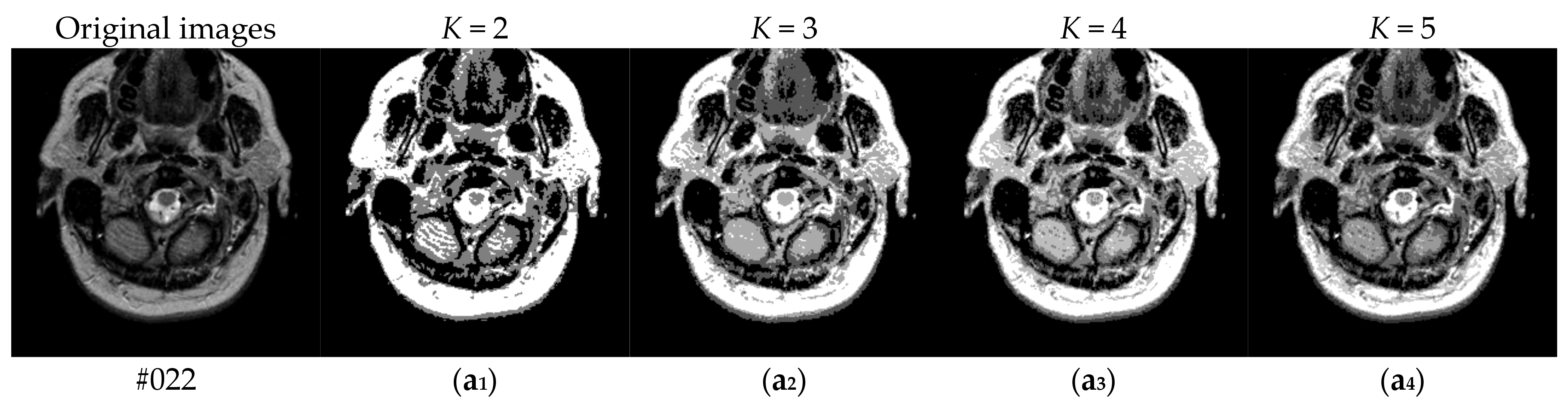
| K = 2, 3, 4, 5 | Number of the thresholds |
| Test Images | Number of Thresholds (K) | Uniformity Measure (U) | |||||
|---|---|---|---|---|---|---|---|
| Proposed | PSO | BF | ABF | NMS | RCGA | ||
| #022 | 2 | 0.9870 | 0.9552 | 0.9569 | 0.9569 | 0.9569 | 0.9569 |
| 3 | 0.9894 | 0.9672 | 0.9708 | 0.9696 | 0.9769 | 0.9769 | |
| 4 | 0.9904 | 0.9420 | 0.9765 | 0.9698 | 0.9824 | 0.9824 | |
| 5 | 0.9917 | 0.9435 | 0.9786 | 0.9785 | 0.9752 | 0.9788 | |
| #032 | 2 | 0.9845 | 0.9368 | 0.9342 | 0.9342 | 0.9342 | 0.9342 |
| 3 | 0.9886 | 0.9619 | 0.9716 | 0.9600 | 0.9796 | 0.9801 | |
| 4 | 0.9891 | 0.9144 | 0.9697 | 0.9766 | 0.9848 | 0.9848 | |
| 5 | 0.9905 | 0.9422 | 0.9668 | 0.9767 | 0.9851 | 0.9843 | |
| #042 | 2 | 0.9827 | 0.9271 | 0.9246 | 0.9246 | 0.9246 | 0.9246 |
| 3 | 0.9812 | 0.9585 | 0.9721 | 0.9689 | 0.9548 | 0.9548 | |
| 4 | 0.9868 | 0.9465 | 0.9752 | 0.9821 | 0.9865 | 0.9865 | |
| 5 | 0.9871 | 0.9348 | 0.9724 | 0.9766 | 0.9845 | 0.9877 | |
| #052 | 2 | 0.9837 | 0.9158 | 0.9128 | 0.9128 | 0.9068 | 0.9128 |
| 3 | 0.9860 | 0.9523 | 0.9713 | 0.9673 | 0.8800 | 0.9467 | |
| 4 | 0.9854 | 0.9372 | 0.9764 | 0.9834 | 0.8982 | 0.9856 | |
| 5 | 0.9880 | 0.9240 | 0.9735 | 0.9782 | 0.9842 | 0.9868 | |
| #062 | 2 | 0.9759 | 0.9192 | 0.9047 | 0.9049 | 0.9015 | 0.9015 |
| 3 | 0.9799 | 0.8777 | 0.9135 | 0.9029 | 0.9030 | 0.9030 | |
| 4 | 0.9849 | 0.9236 | 0.8856 | 0.8988 | 0.8989 | 0.8989 | |
| 5 | 0.9851 | 0.8505 | 0.9527 | 0.9325 | 0.9835 | 0.9855 | |
| #072 | 2 | 0.9723 | 0.9068 | 0.9041 | 0.9041 | 0.9041 | 0.9041 |
| 3 | 0.9788 | 0.9034 | 0.9084 | 0.8985 | 0.8992 | 0.8992 | |
| 4 | 0.9830 | 0.8809 | 0.8876 | 0.8804 | 0.8666 | 0.8666 | |
| 5 | 0.9878 | 0.9531 | 0.8881 | 0.8876 | 0.9818 | 0.9825 | |
| #082 | 2 | 0.9782 | 0.9120 | 0.9091 | 0.9091 | 0.9091 | 0.9091 |
| 3 | 0.9734 | 0.8852 | 0.8621 | 0.8661 | 0.8849 | 0.8849 | |
| 4 | 0.9816 | 0.8619 | 0.8479 | 0.8622 | 0.8695 | 0.8695 | |
| 5 | 0.9847 | 0.9372 | 0.9188 | 0.9105 | 0.9854 | 0.9857 | |
| #092 | 2 | 0.9870 | 0.9131 | 0.9156 | 0.9131 | 0.9131 | 0.9131 |
| 3 | 0.9877 | 0.8607 | 0.8751 | 0.8827 | 0.8786 | 0.8786 | |
| 4 | 0.9863 | 0.9490 | 0.8583 | 0.8514 | 0.8240 | 0.8641 | |
| 5 | 0.9887 | 0.8684 | 0.8923 | 0.8401 | 0.9880 | 0.9876 | |
| #102 | 2 | 0.9864 | 0.9383 | 0.9250 | 0.9250 | 0.9250 | 0.9250 |
| 3 | 0.9851 | 0.8768 | 0.8977 | 0.9097 | 0.9179 | 0.9179 | |
| 4 | 0.9888 | 0.9256 | 0.9410 | 0.9050 | 0.9871 | 0.9871 | |
| 5 | 0.9921 | 0.8446 | 0.9180 | 0.9181 | 0.9907 | 0.9895 | |
| #112 | 2 3 4 5 | 0.9875 | 0.9356 | 0.9403 | 0.9404 | 0.9404 | 0.9404 |
| 0.9906 | 0.9147 | 0.9666 | 0.9769 | 0.9863 | 0.9890 | ||
| 0.9899 | 0.9751 | 0.9824 | 0.9825 | 0.9885 | 0.9896 | ||
| 0.9887 | 0.9735 | 0.9822 | 0.9830 | 0.9915 | 0.9914 | ||
| Test Images | Number of Thresholds (K) | Optimal Threshold Values | |||||
|---|---|---|---|---|---|---|---|
| Proposed | PSO | BF | ABF | NMS | RCGA | ||
| #022 | 2 | 33, 92 | 97, 184 | 96, 184 | 95, 184 | 96, 184 | 96, 184 |
| 3 | 17, 56, 110 | 69, 138, 207 | 65, 131, 186 | 69, 114, 185 | 58, 116, 185 | 58, 115, 185 | |
| 4 | 13, 37, 74, 116 | 83, 116, 175, 207 | 52, 99, 148, 186 | 58, 113, 174, 208 | 43, 87, 132, 185 | 44, 87, 131, 186 | |
| 5 | 13, 37, 74, 108, 134 | 76, 119, 154, 184, 214 | 44, 90, 127, 170, 208 | 43, 88, 130, 176, 208 | 44, 104, 140, 176, 214 | 44, 86, 127, 174, 208 | |
| #032 | 2 | 32,90 | 107, 185 | 110, 185 | 110, 185 | 110, 185 | 109, 185 |
| 3 | 24, 70, 116 | 74, 157, 192 | 72, 120, 198 | 81, 134, 187 | 56, 115, 186 | 53, 116, 185 | |
| 4 | 13, 43, 87, 127 | 95, 125, 164, 194 | 63, 119, 173, 208 | 58, 102, 142, 190 | 39, 83, 132, 189 | 39, 84, 131, 189 | |
| 5 | 11, 37, 67, 94, 125 | 80, 112, 139, 186, 213 | 63, 101, 140, 175, 207 | 52, 87, 128, 167, 198 | 29, 75, 124, 173, 207 | 34, 78, 123, 174, 207 | |
| #042 | 2 | 46, 107 | 111, 183 | 114, 184 | 114, 184 | 113, 184 | 114, 183 |
| 3 | 18, 60, 107 | 80, 148, 178 | 70, 136, 188 | 74, 130, 185 | 84, 132, 188 | 84, 132, 187 | |
| 4 | 18, 58, 100, 140 | 81, 125, 164, 197 | 62, 112, 156, 194 | 50, 100, 143, 190 | 29, 76, 128, 187 | 30, 75, 127, 188 | |
| 5 | 18, 55, 86, 112, 142 | 82, 115, 142, 184, 214 | 58, 114, 151, 188, 218 | 53, 97, 144, 184, 218 | 31, 76, 126, 178, 217 | 25, 69, 114, 156, 194 | |
| #052 | 2 | 48, 97 | 119, 186 | 117, 186 | 117, 186 | 118, 185 | 118, 185 |
| 3 | 44, 87, 122 | 89, 113, 187 | 102, 156, 206 | 107, 158, 204 | 109, 166, 207 | 109, 165, 203 | |
| 4 | 42, 80, 105, 130 | 79, 111, 141, 208 | 93, 124, 171, 210 | 90, 129, 173, 210 | 94, 132, 175, 210 | 91, 131, 174, 209 | |
| 5 | 26, 55, 80, 105, 130 | 65, 85, 131, 162, 203 | 56, 112, 144, 175, 209 | 56, 95, 133, 167, 203 | 20, 67, 120, 167, 207 | 24, 67, 118, 166, 203 | |
| #062 | 2 | 66, 109 | 109, 186 | 119, 190 | 119, 186 | 121, 187 | 121, 187 |
| 3 | 53, 89, 125 | 112, 167, 187 | 97, 133, 183 | 102, 147, 199 | 101, 148, 195 | 101, 147, 196 | |
| 4 | 33, 76, 108, 149 | 85, 134, 180, 203 | 98, 140, 182, 218 | 93, 135, 175, 212 | 94, 134, 176, 211 | 94, 134, 175, 211 | |
| 5 | 33, 76, 98, 125, 156 | 99, 119, 157, 181, 203 | 73, 104, 139, 184, 213 | 79, 111, 145, 179, 212 | 28, 68, 120, 168, 208 | 20, 65, 113, 158, 200 | |
| #072 | 2 | 47, 91 | 116, 177 | 117, 179 | 117, 179 | 118, 179 | 117, 179 |
| 3 | 47, 89, 123 | 96, 178, 207 | 95, 147, 202 | 99, 150, 190 | 100, 142, 188 | 99, 141, 187 | |
| 4 | 25, 73, 106, 145 | 96, 124, 161, 187 | 94, 129, 173, 214 | 95, 134, 174, 214 | 100, 140, 179, 214 | 99, 140, 179, 213 | |
| 5 | 25, 72, 99, 129, 174 | 72, 112, 151, 178, 197 | 87, 109, 139, 178, 210 | 87, 119, 150, 180, 214 | 10, 64, 120, 172, 211 | 14, 64, 119, 171, 211 | |
| #082 | 2 | 48, 96 | 110, 170 | 112, 169 | 111, 170 | 112, 169 | 111, 169 |
| 3 | 20, 72, 100 | 103, 136, 198 | 114, 155, 210 | 111, 155, 201 | 103, 146, 189 | 103, 146, 190 | |
| 4 | 20, 72, 98, 134 | 100, 129, 167, 188 | 103, 139, 175, 214 | 99, 135, 170, 210 | 98, 134, 169, 210 | 98, 133, 169, 210 | |
| 5 | 20, 72, 94, 116, 152 | 78, 105, 151, 180, 201 | 81, 122, 150, 182, 212 | 84, 113, 146, 178, 214 | 14, 62, 115, 168, 210 | 10, 62, 107, 148, 190 | |
| #092 | 2 | 58, 98 | 109, 175 | 108, 174 | 109, 174 | 109, 173 | 109, 174 |
| 3 | 35, 79, 107 | 115, 134, 178 | 107, 144, 209 | 104, 158, 207 | 106, 158, 206 | 105, 158, 206 | |
| 4 | 24, 63, 83, 107 | 77, 107, 149, 194 | 100, 129, 164, 208 | 102, 138, 171, 212 | 112, 152, 186, 220 | 97, 136, 211, 173 | |
| 5 | 24, 63, 82, 101, 121 | 90, 113, 165, 185, 206 | 85, 114, 147, 175, 212 | 96, 128, 158, 186, 216 | 10, 64, 110, 160, 205 | 5, 62, 109, 159, 205 | |
| #102 | 2 | 55, 97 | 98, 166 | 108, 174 | 108, 174 | 108, 173 | 107, 174 |
| 3 | 25, 64, 97 | 113, 145, 180 | 103, 148, 189 | 98, 146, 189 | 94, 142, 189 | 94, 142, 190 | |
| 4 | 25, 62, 86, 118 | 84, 124, 165, 189 | 79, 122, 164, 200 | 90, 127, 164, 198 | 2, 64, 119, 173 | 1, 63, 120, 174 | |
| 5 | 25, 62, 86, 112, 140 | 99, 128, 147, 194, 218 | 81, 113, 147, 187, 220 | 82, 114, 148, 184, 218 | 9, 62, 106, 147, 190 | 1, 62, 104, 145, 189 | |
| #112 | 2 | 54, 100 | 109, 162 | 105, 165 | 105, 164 | 106, 163 | 106, 163 |
| 3 | 29, 76, 111 | 104, 163, 216 | 79, 134, 180 | 71, 123, 175 | 3, 49, 145 | 1, 70, 142 | |
| 4 | 25, 61, 90, 111 | 63, 130, 153, 206 | 54, 117, 156, 192 | 58, 105, 146, 182 | 4, 63, 132, 178 | 1, 65, 123, 172 | |
| 5 | 18, 49, 76, 94, 111 | 58, 128, 155, 187, 213 | 48, 112, 137, 161, 200 | 47, 108, 142, 171, 197 | 2, 44, 79, 131, 175 | 1, 49, 95, 139, 183 | |
| Number of Thresholds (K) | Average Uniformity Measure (U) | |||
|---|---|---|---|---|
| Non-F-RGM | F-RGM | Non-F-RGIIM | Proposed | |
| 2 | 0.9696 | 0.9729 | 0.9795 | 0.9825 |
| 3 | 0.9723 | 0.9775 | 0.9838 | 0.9840 |
| 4 | 0.9677 | 0.9820 | 0.9864 | 0.9866 |
| 5 | 0.9791 | 0.9850 | 0.9877 | 0.9884 |
| Methods | Proposed | PSO | BF | ABF | NMS | RCGA |
|---|---|---|---|---|---|---|
| 1 K pixel/s | 0.008 | 0.1057 | 0.2772 | 0.3254 | 0.3548 | 0.2815 |
Disclaimer/Publisher’s Note: The statements, opinions and data contained in all publications are solely those of the individual author(s) and contributor(s) and not of MDPI and/or the editor(s). MDPI and/or the editor(s) disclaim responsibility for any injury to people or property resulting from any ideas, methods, instructions or products referred to in the content. |
© 2023 by the authors. Licensee MDPI, Basel, Switzerland. This article is an open access article distributed under the terms and conditions of the Creative Commons Attribution (CC BY) license (https://creativecommons.org/licenses/by/4.0/).
Share and Cite
Feng, Y.; Liu, Y.; Liu, Z.; Liu, W.; Yao, Q.; Zhang, X. A Novel Interval Iterative Multi-Thresholding Algorithm Based on Hybrid Spatial Filter and Region Growing for Medical Brain MR Images. Appl. Sci. 2023, 13, 1087. https://doi.org/10.3390/app13021087
Feng Y, Liu Y, Liu Z, Liu W, Yao Q, Zhang X. A Novel Interval Iterative Multi-Thresholding Algorithm Based on Hybrid Spatial Filter and Region Growing for Medical Brain MR Images. Applied Sciences. 2023; 13(2):1087. https://doi.org/10.3390/app13021087
Chicago/Turabian StyleFeng, Yuncong, Yunfei Liu, Zhicheng Liu, Wanru Liu, Qingan Yao, and Xiaoli Zhang. 2023. "A Novel Interval Iterative Multi-Thresholding Algorithm Based on Hybrid Spatial Filter and Region Growing for Medical Brain MR Images" Applied Sciences 13, no. 2: 1087. https://doi.org/10.3390/app13021087
APA StyleFeng, Y., Liu, Y., Liu, Z., Liu, W., Yao, Q., & Zhang, X. (2023). A Novel Interval Iterative Multi-Thresholding Algorithm Based on Hybrid Spatial Filter and Region Growing for Medical Brain MR Images. Applied Sciences, 13(2), 1087. https://doi.org/10.3390/app13021087