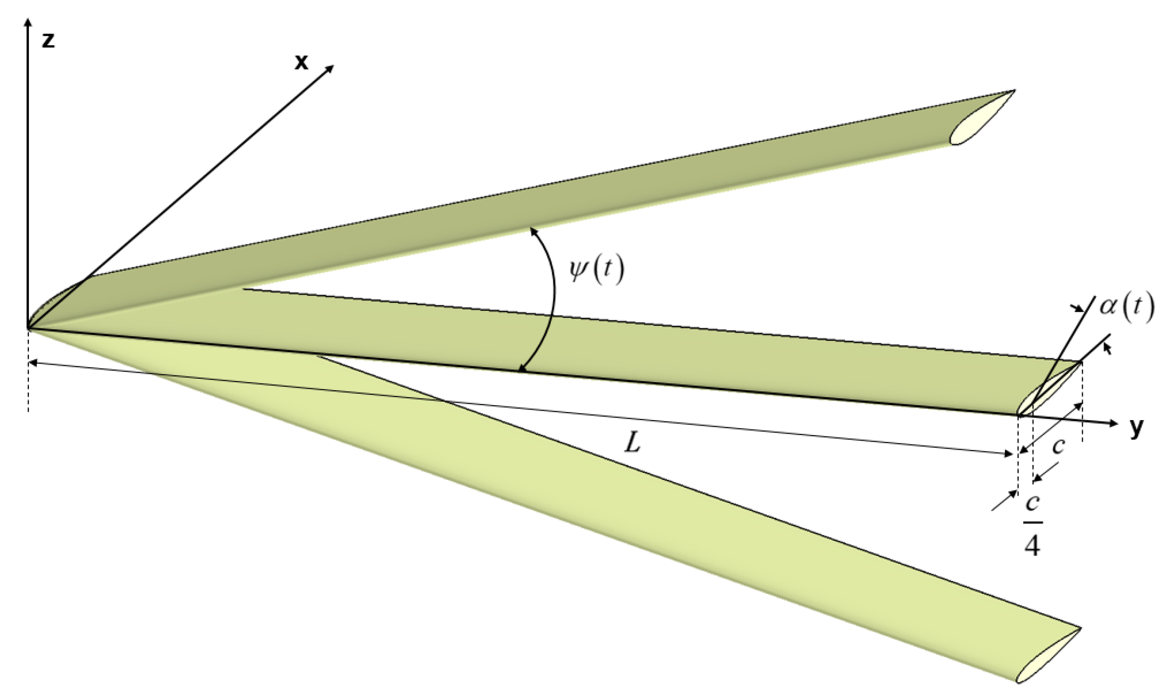
Figure 1.
Motion of flapping wing.
Figure 1.
Motion of flapping wing.
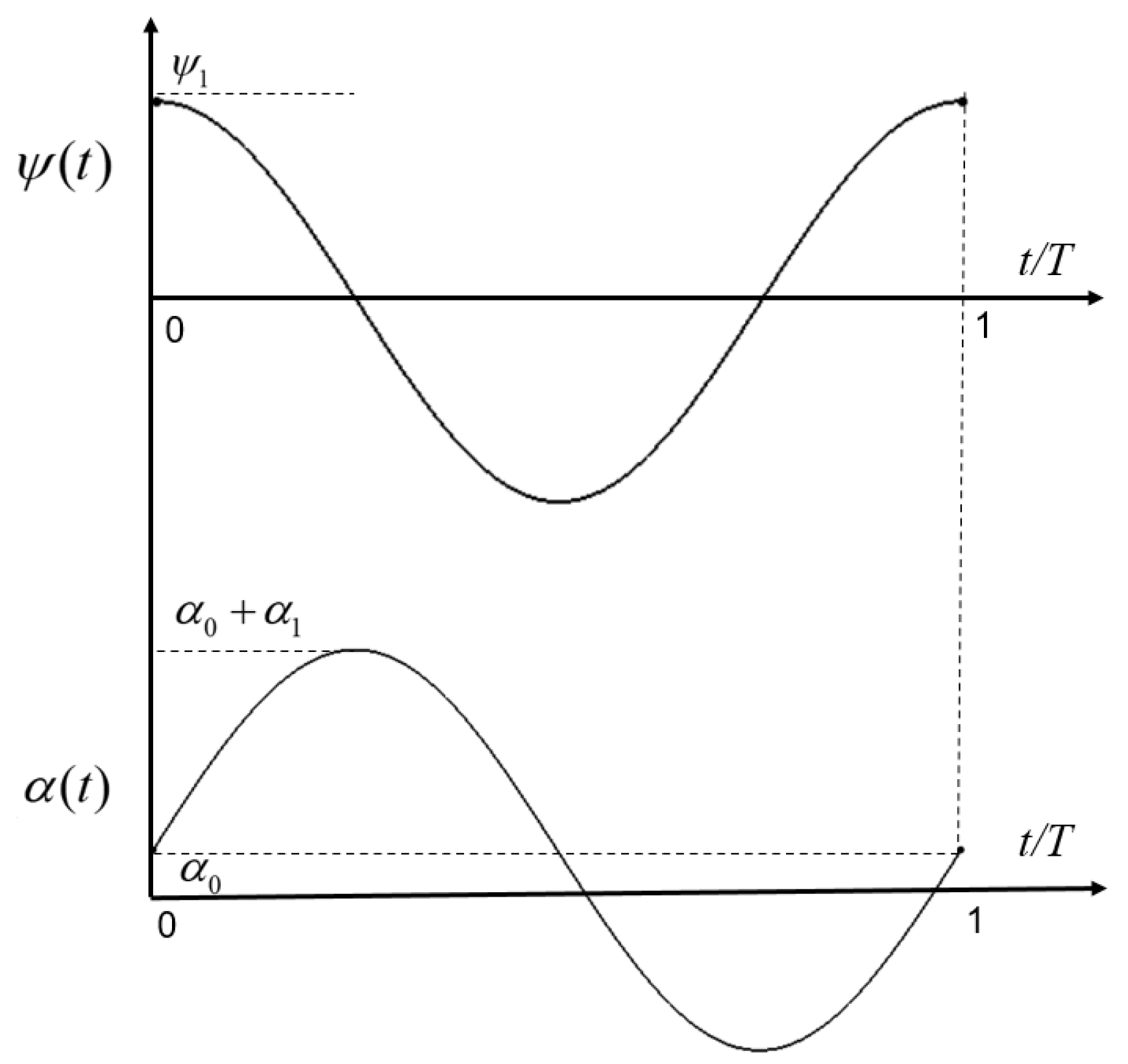
Figure 2.
The time history plot corresponding to Equation (1).
Figure 2.
The time history plot corresponding to Equation (1).
Figure 3.
Comparison of average lift coefficient.
Figure 3.
Comparison of average lift coefficient.
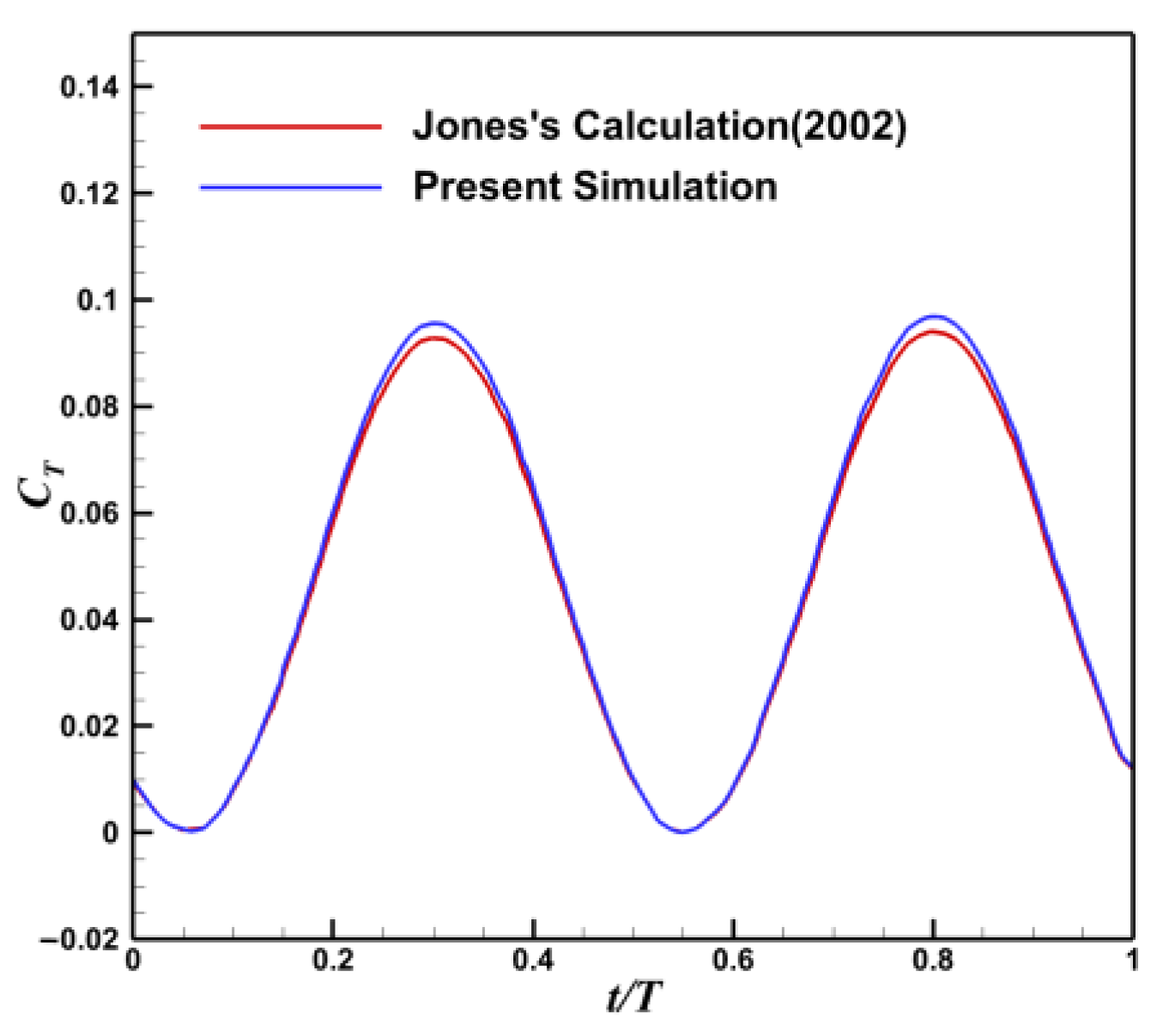
Figure 4.
Comparison of average thrust coefficient.
Figure 4.
Comparison of average thrust coefficient.
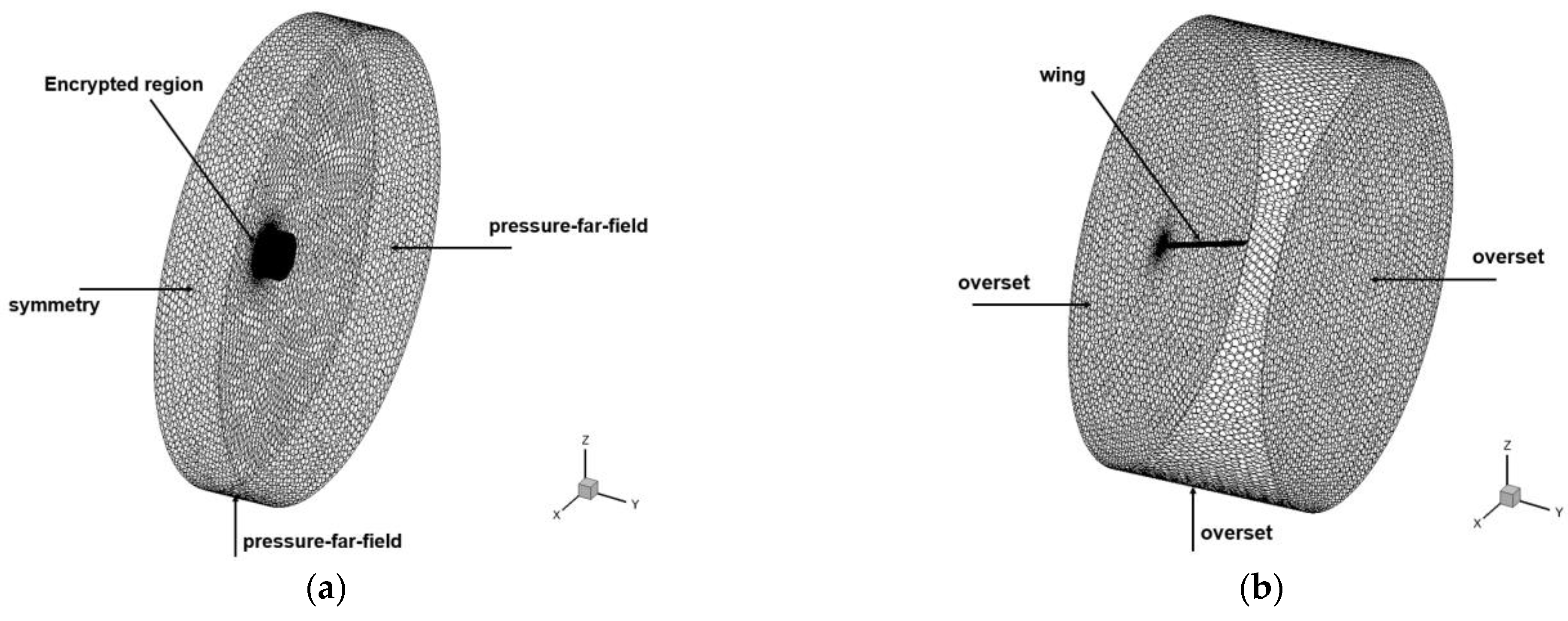
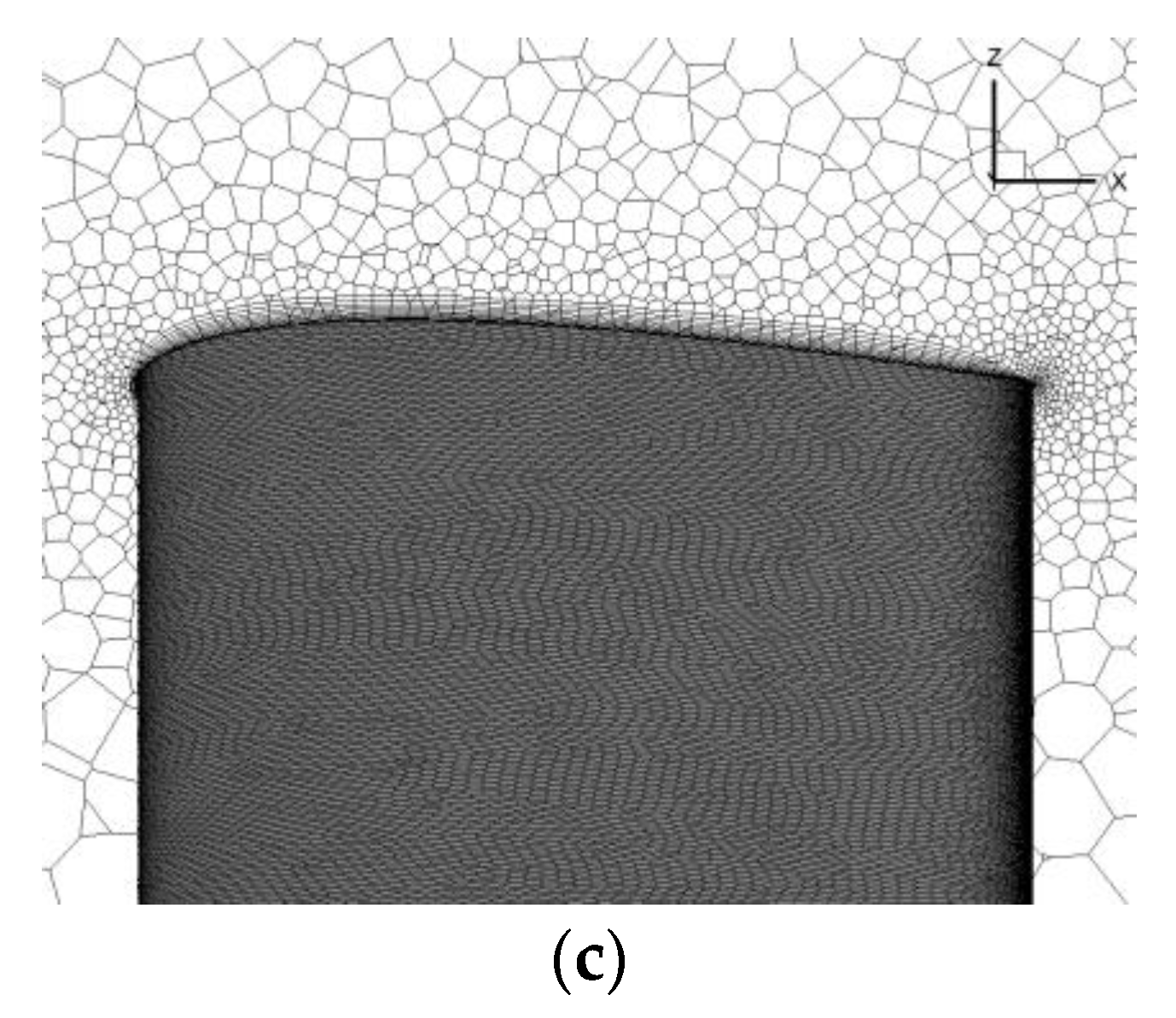
Figure 5.
Grid and boundary conditions. (a) Background grid; (b) Component grid; (c) Boundary layer and surface mesh.
Figure 5.
Grid and boundary conditions. (a) Background grid; (b) Component grid; (c) Boundary layer and surface mesh.
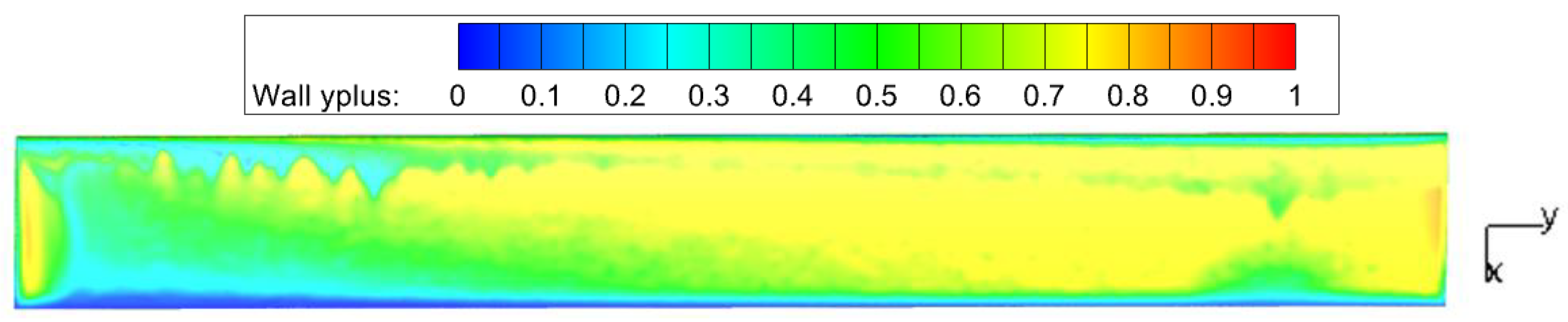
Figure 6.
The y+ contours of baseline case.
Figure 6.
The y+ contours of baseline case.
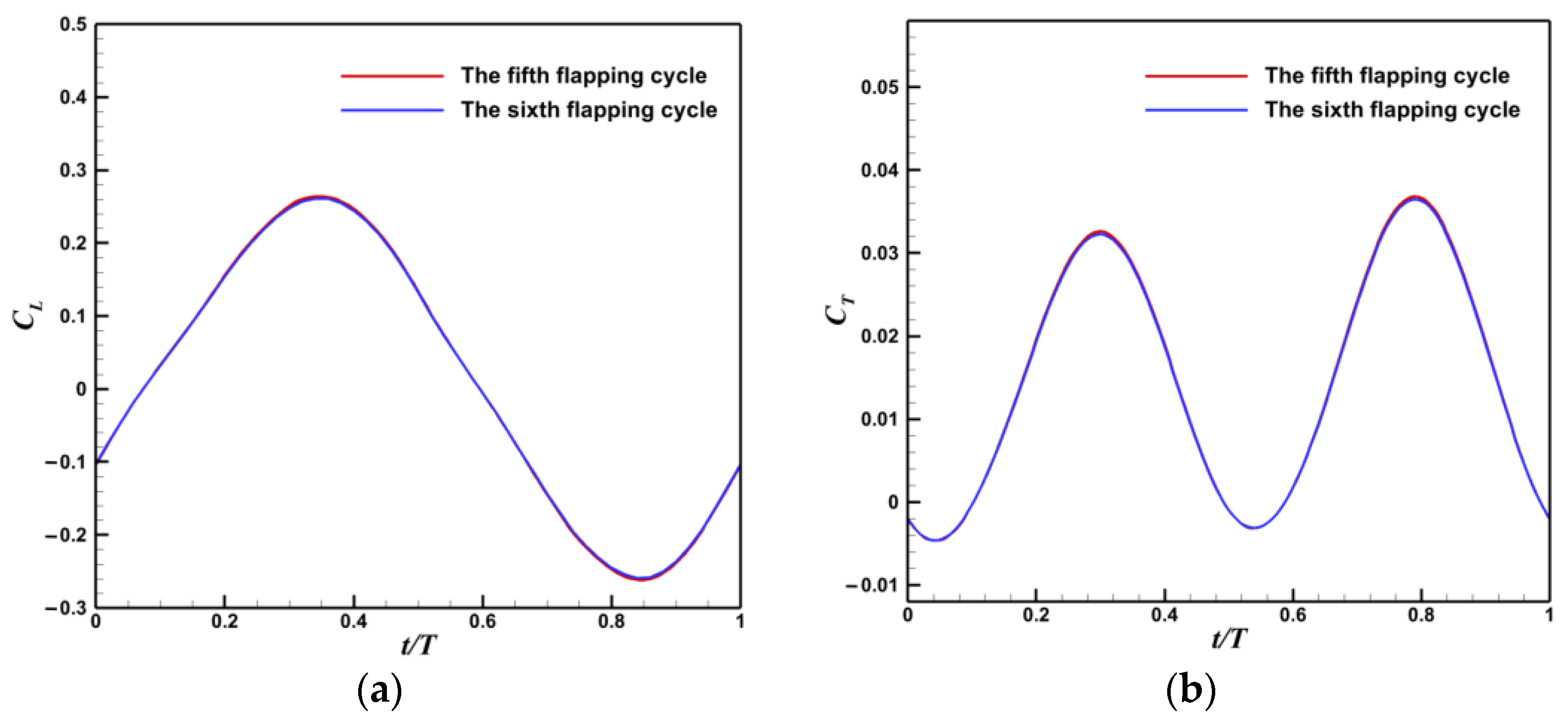
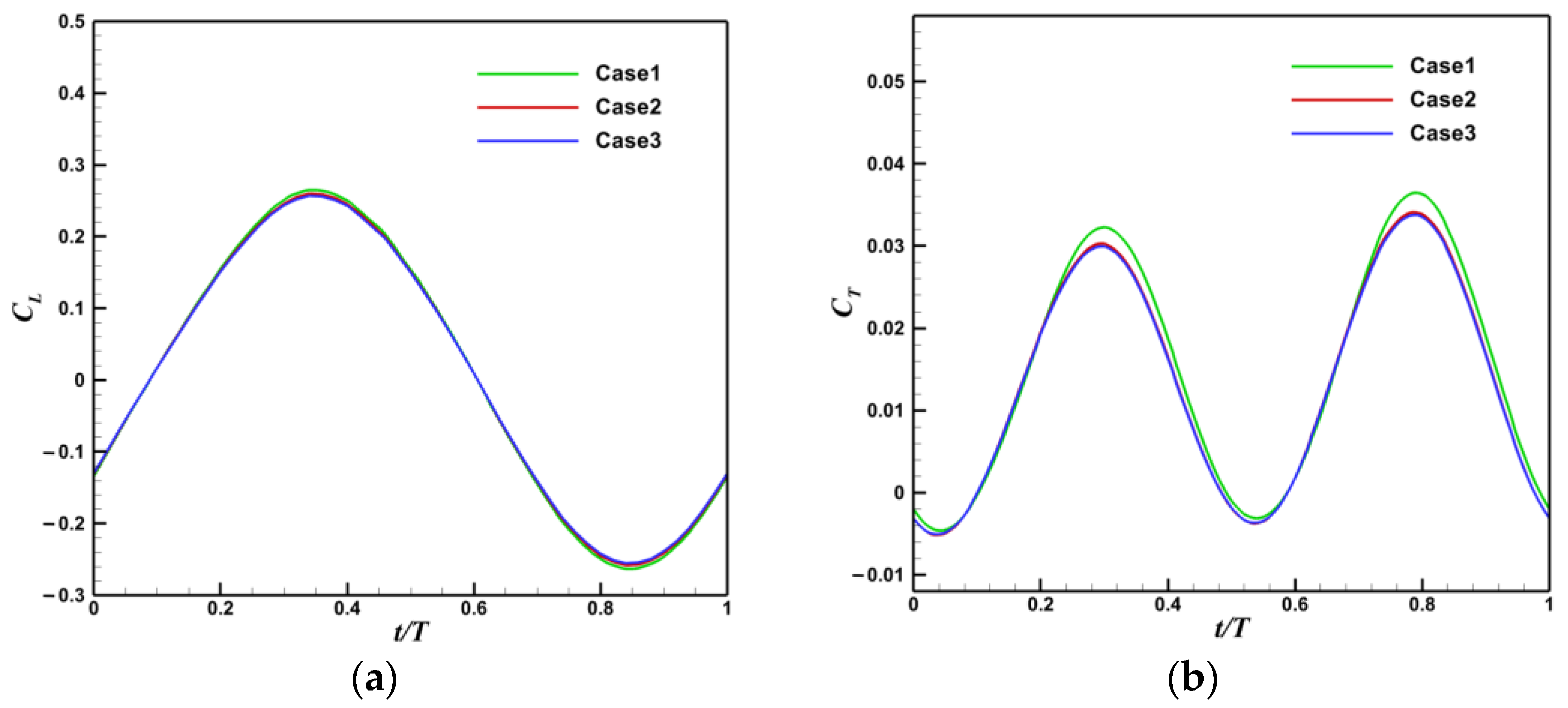
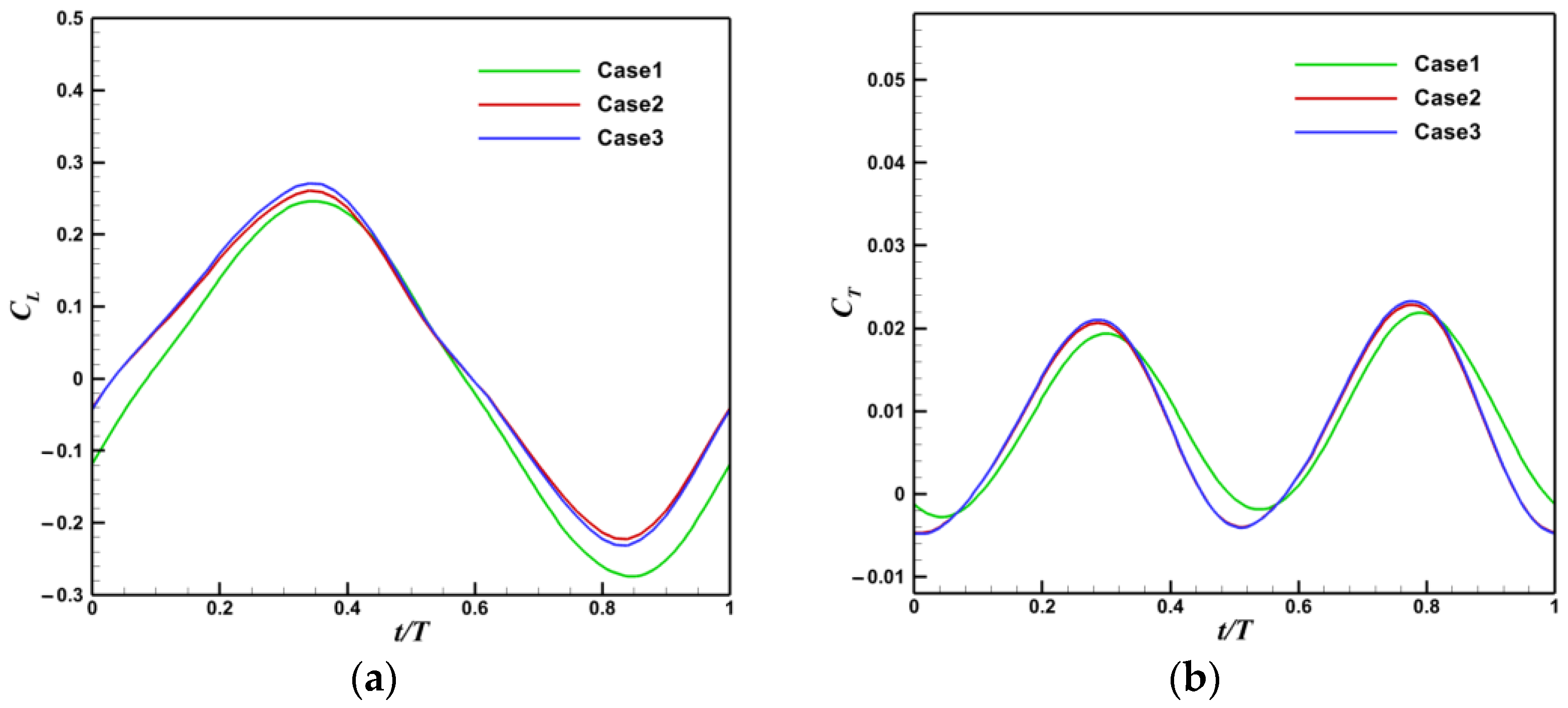
Figure 7.
The comparison of time history of lift and thrust coefficient. (a) Lift coefficient; (b) Trust coefficient.
Figure 7.
The comparison of time history of lift and thrust coefficient. (a) Lift coefficient; (b) Trust coefficient.
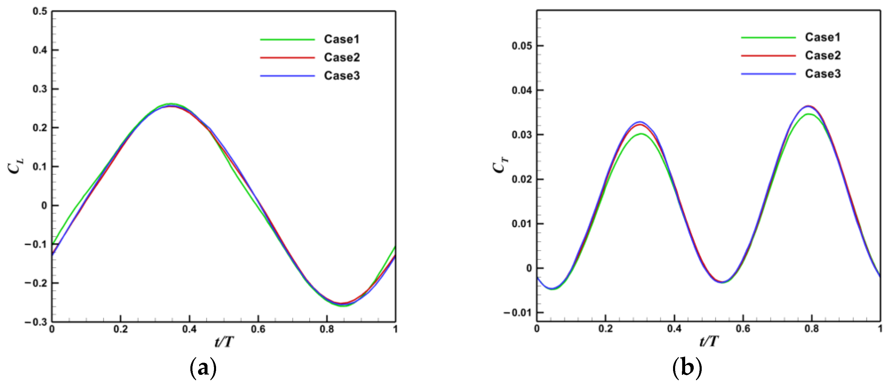
Figure 8.
Grid independence verification. (a) Lift coefficient; (b) Trust coefficient.
Figure 8.
Grid independence verification. (a) Lift coefficient; (b) Trust coefficient.
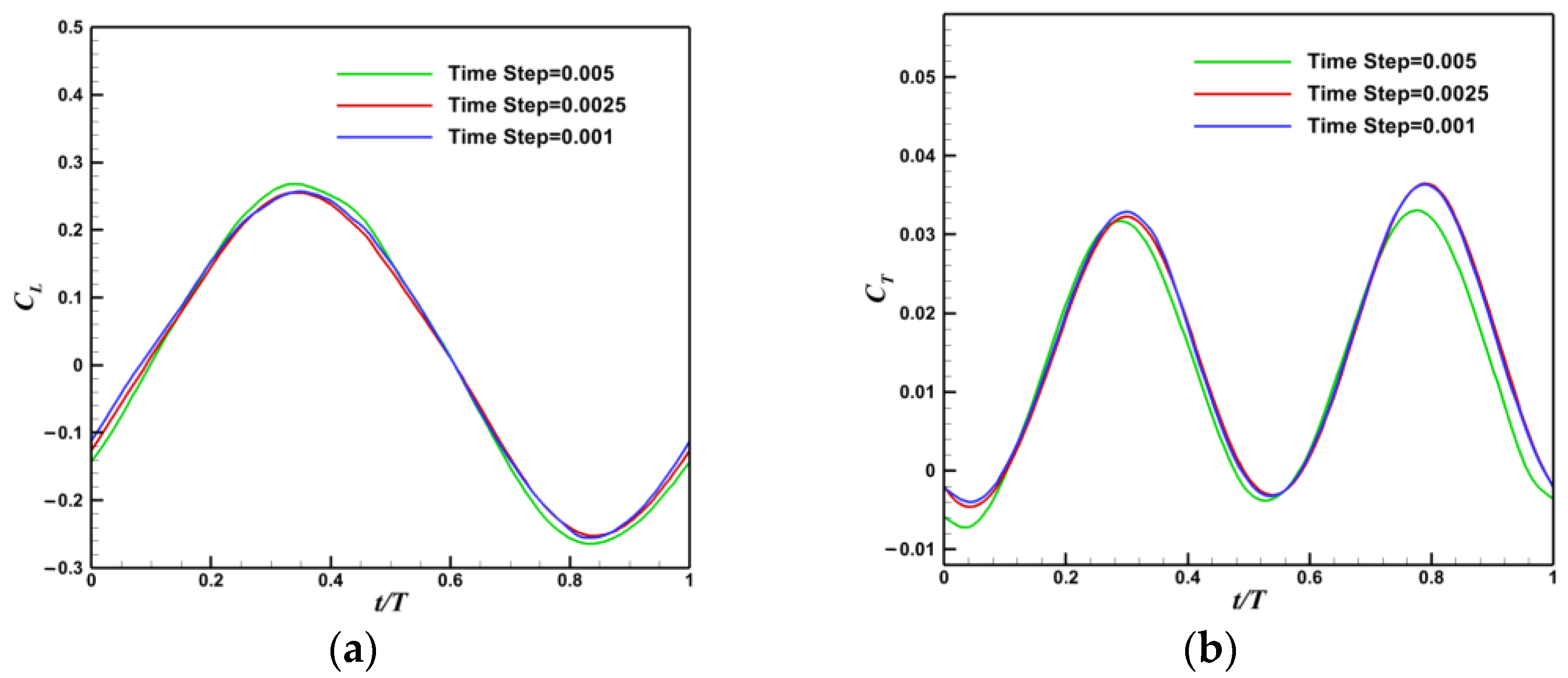
Figure 9.
Time step independence verification. (a) Lift coefficient; (b) Trust coefficient.
Figure 9.
Time step independence verification. (a) Lift coefficient; (b) Trust coefficient.
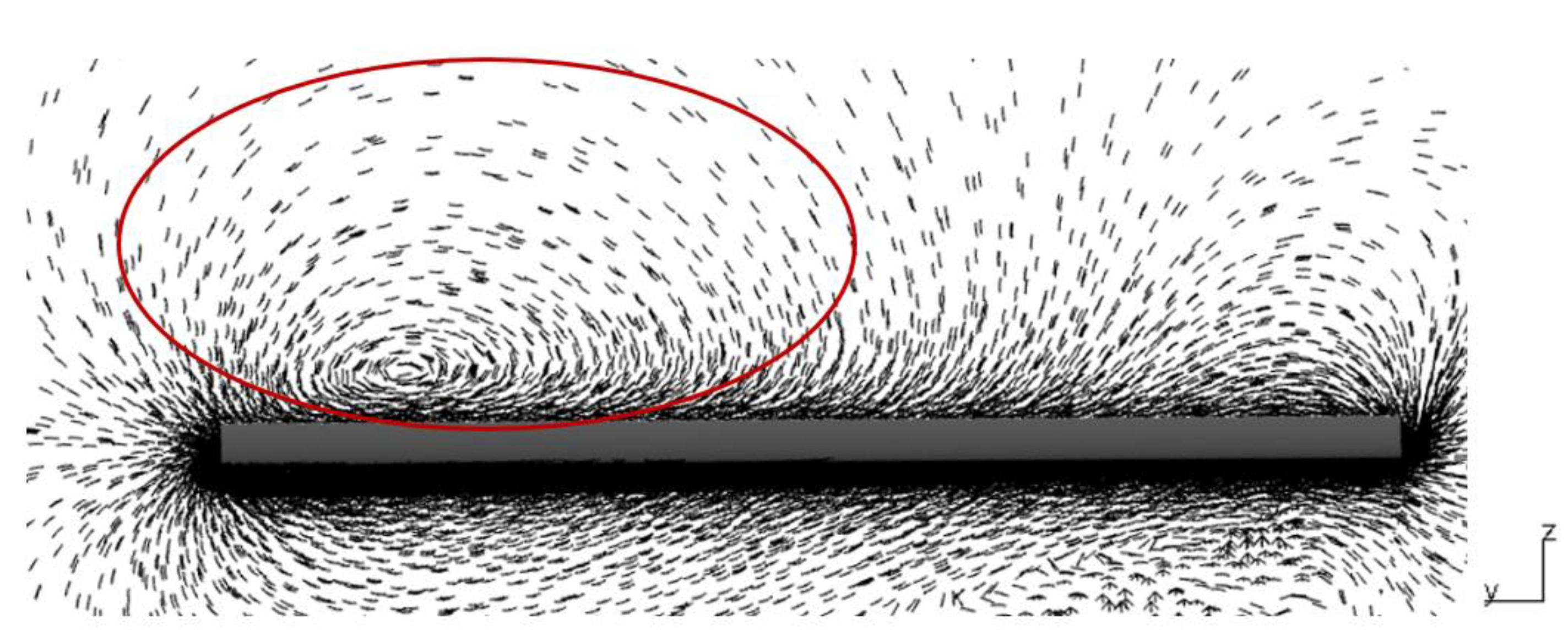
Figure 10.
Velocity vector diagram of 1% chordwise section at t/T = 0.25.
Figure 10.
Velocity vector diagram of 1% chordwise section at t/T = 0.25.
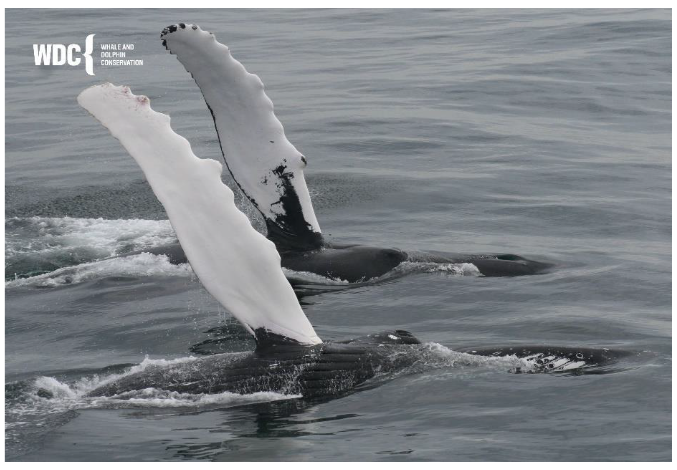
Figure 11.
Flipper’s front structure of humpback whale [
41].
Figure 11.
Flipper’s front structure of humpback whale [
41].
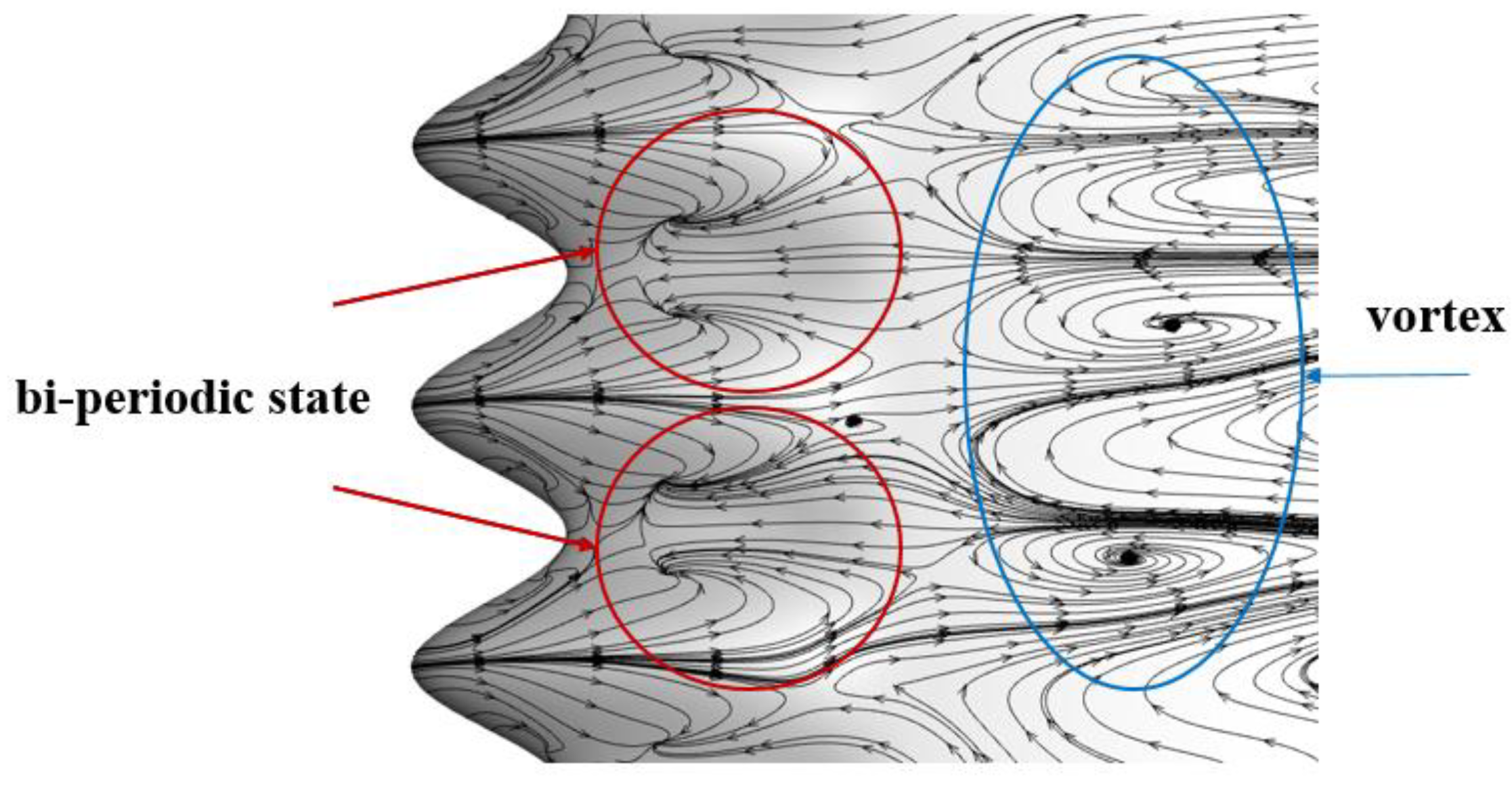
Figure 12.
Upper surface limit streamline of wavy leading edge wing.
Figure 12.
Upper surface limit streamline of wavy leading edge wing.
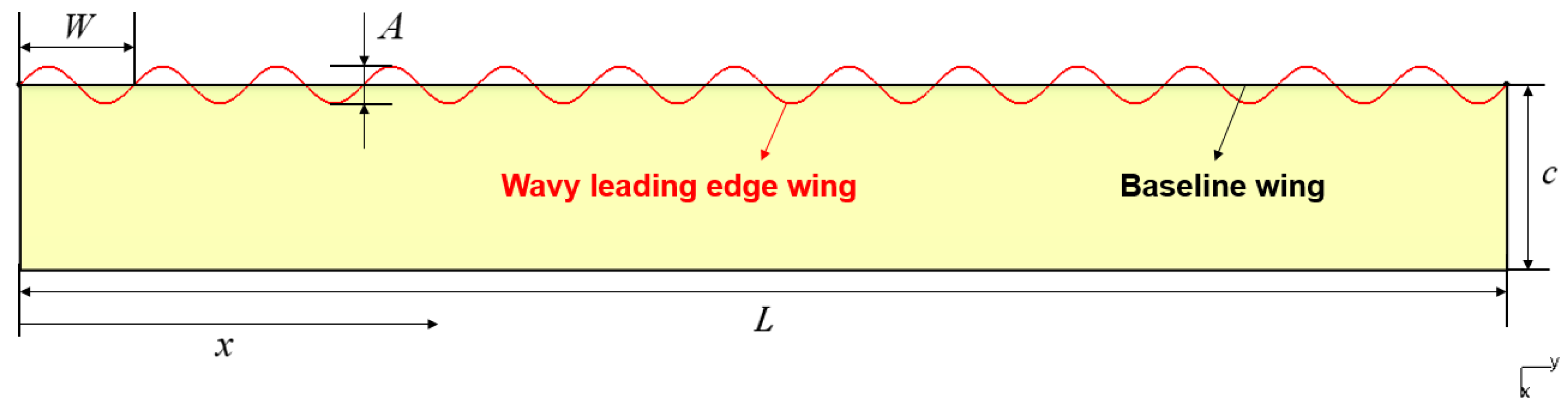
Figure 13.
Wavy leading edge wing.
Figure 13.
Wavy leading edge wing.
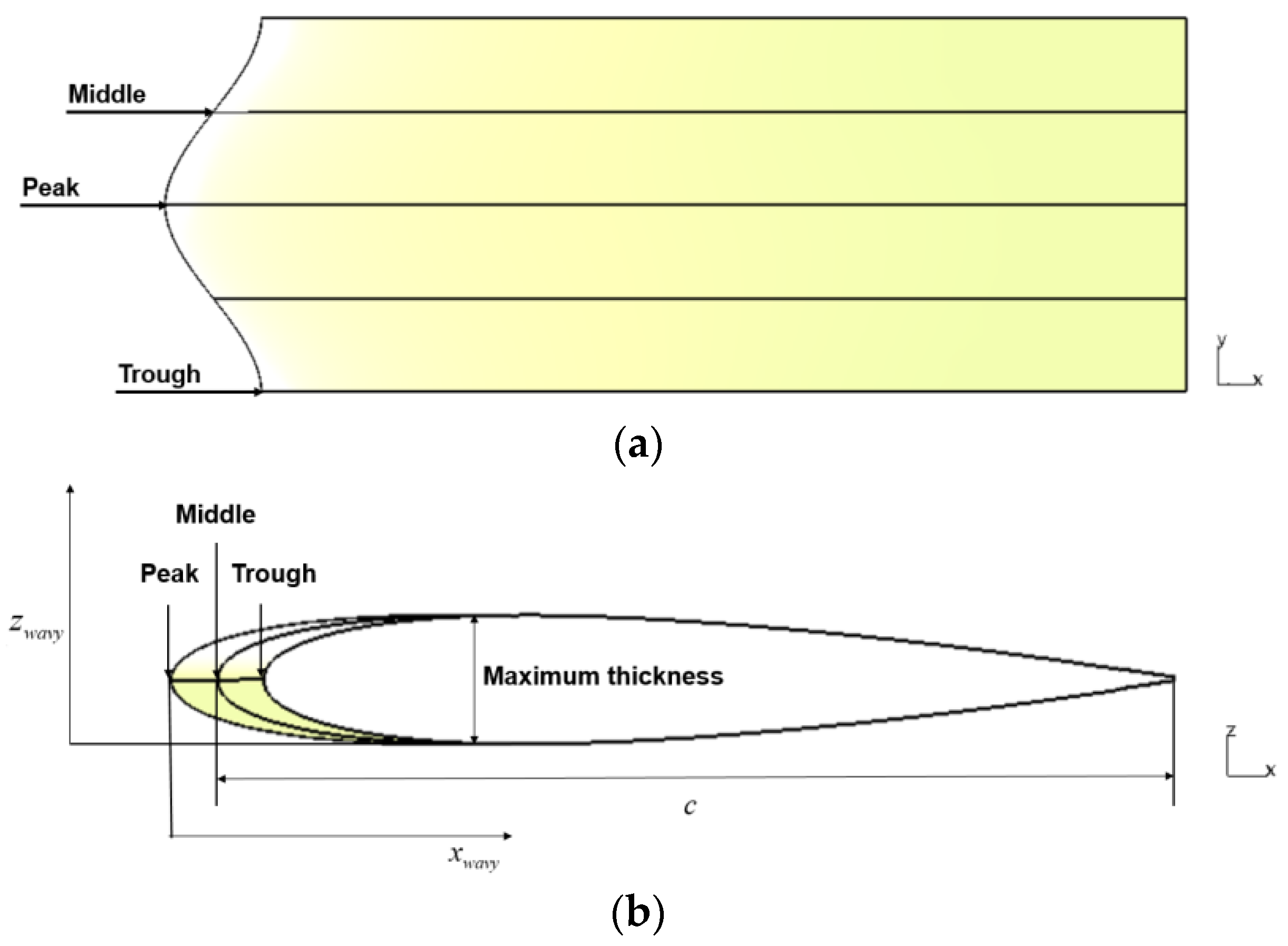
Figure 14.
Construction method of wavy leading edge wing. (a) Wing spanwise section of wavy leading edge wing; (b) Airfoil of wavy leading edge wing.
Figure 14.
Construction method of wavy leading edge wing. (a) Wing spanwise section of wavy leading edge wing; (b) Airfoil of wavy leading edge wing.
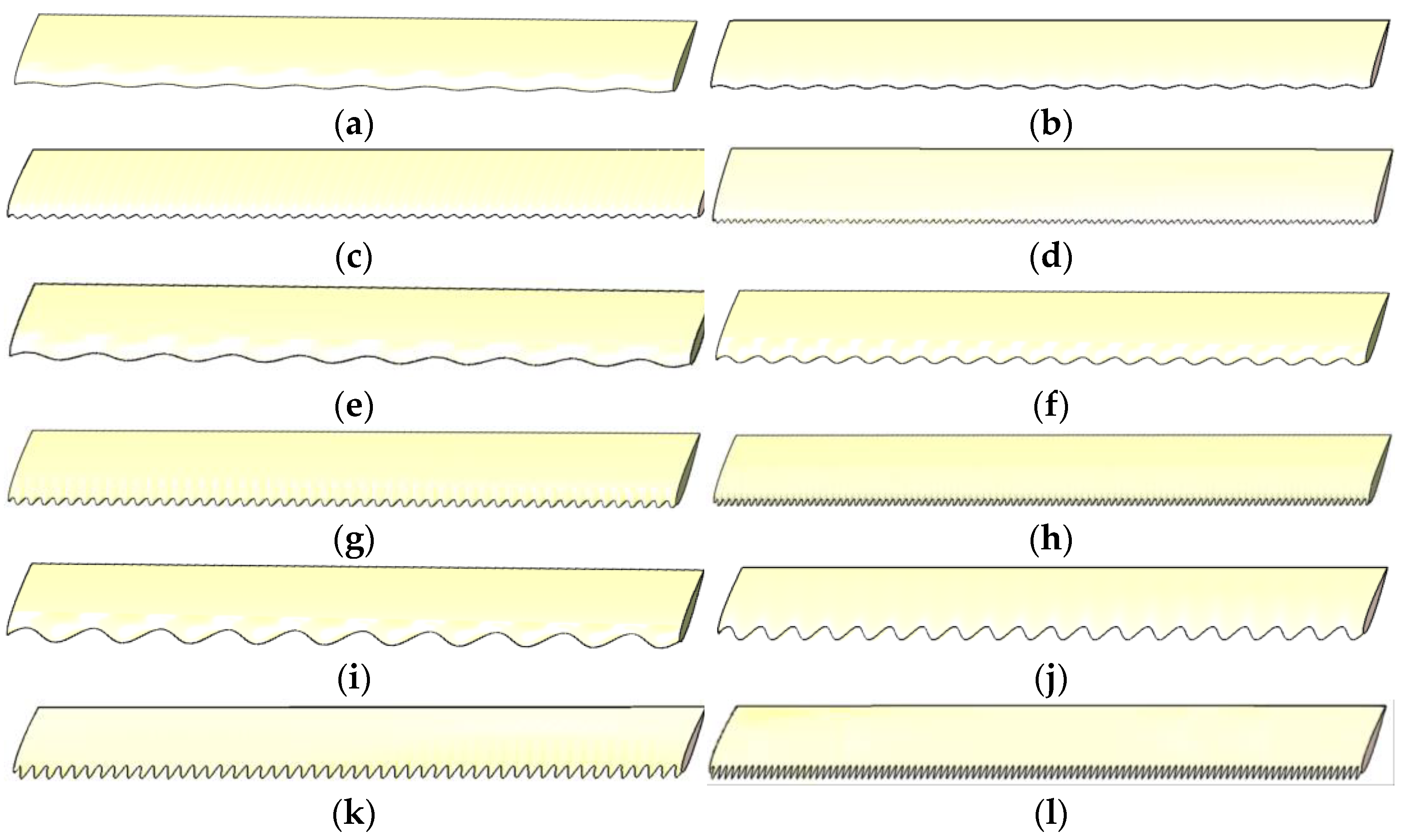
Figure 15.
Wavy leading edge flapping wing configuration. (a) Configuration 1-1; (b) Configuration 1-2; (c) Configuration 1-3; (d) Configuration 1-4; (e) Configuration 2-1; (f) Configuration 2-4; (g) Configuration 1-3; (h) Configuration 2-4; (i) Configuration 3-1; (j) Configuration 3-2; (k) Configuration 3-3; (l) Configuration 3-4.
Figure 16.
The time history of lift and thrust coefficient (Configuration 11). (a) Lift coefficient; (b) Trust coefficient.
Figure 16.
The time history of lift and thrust coefficient (Configuration 11). (a) Lift coefficient; (b) Trust coefficient.
Figure 17.
The time history of lift and thrust coefficient (Configuration 3-4). (a) Lift coefficient; (b) Trust coefficient.
Figure 17.
The time history of lift and thrust coefficient (Configuration 3-4). (a) Lift coefficient; (b) Trust coefficient.
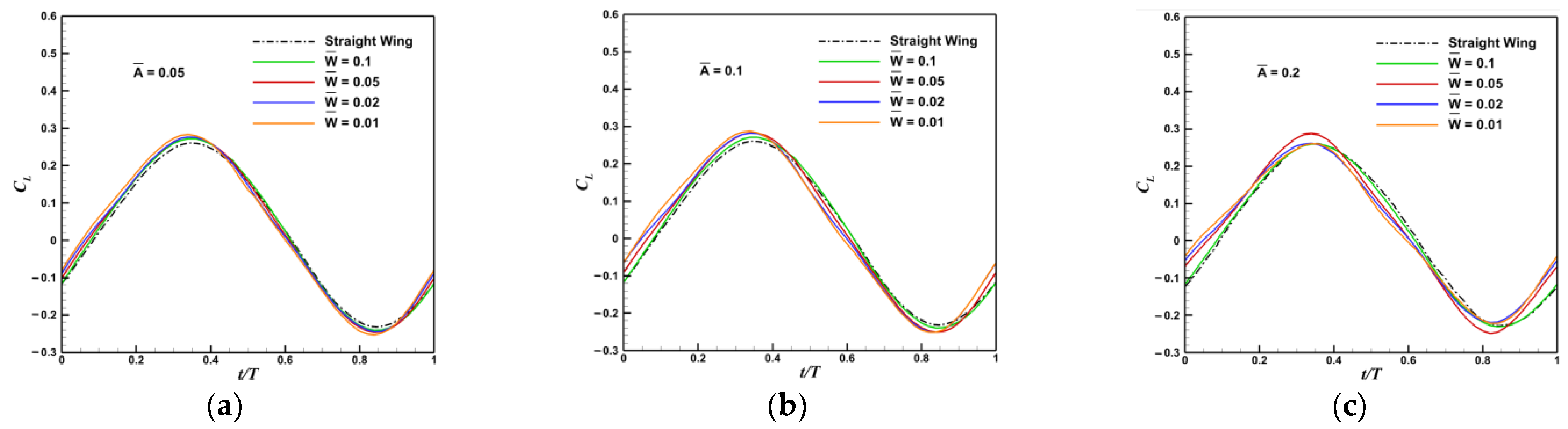
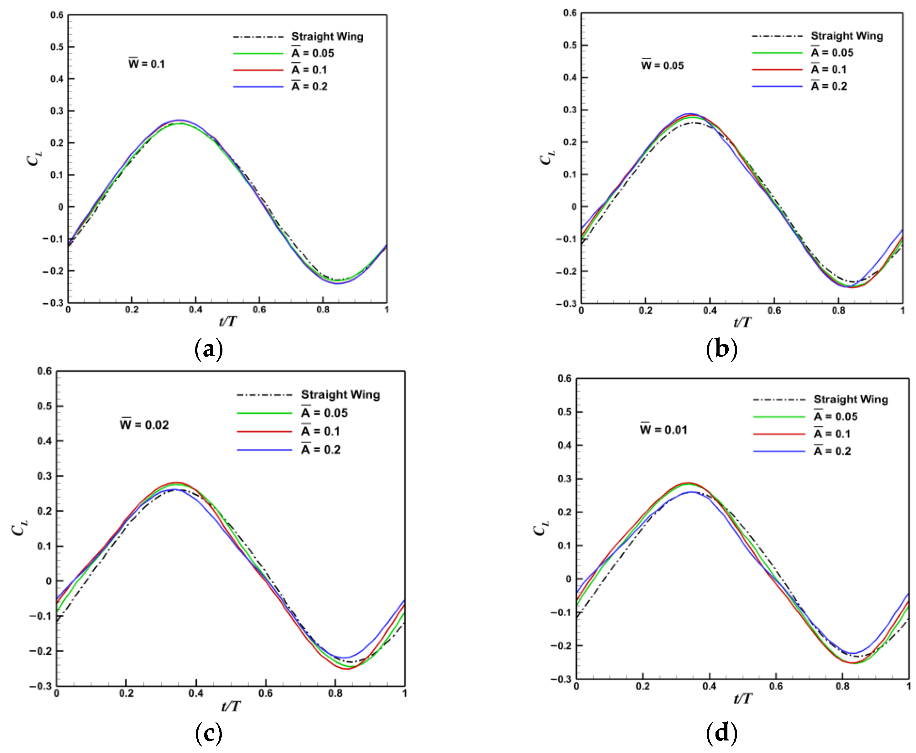
Figure 18.
Time history of lift coefficient in a flapping cycle. (a) ; (b) ; (c) .
Figure 18.
Time history of lift coefficient in a flapping cycle. (a) ; (b) ; (c) .
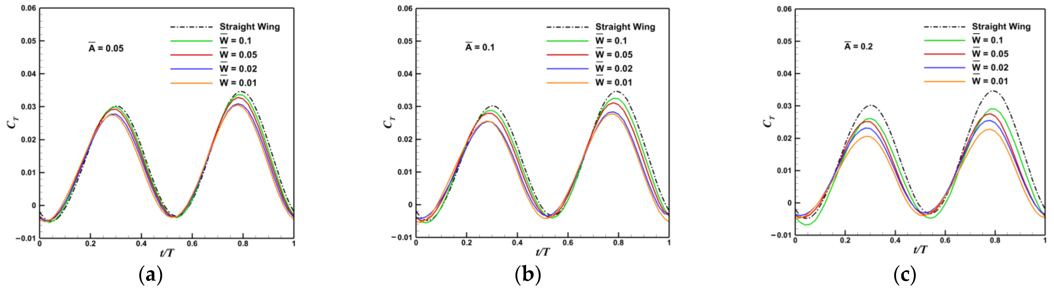
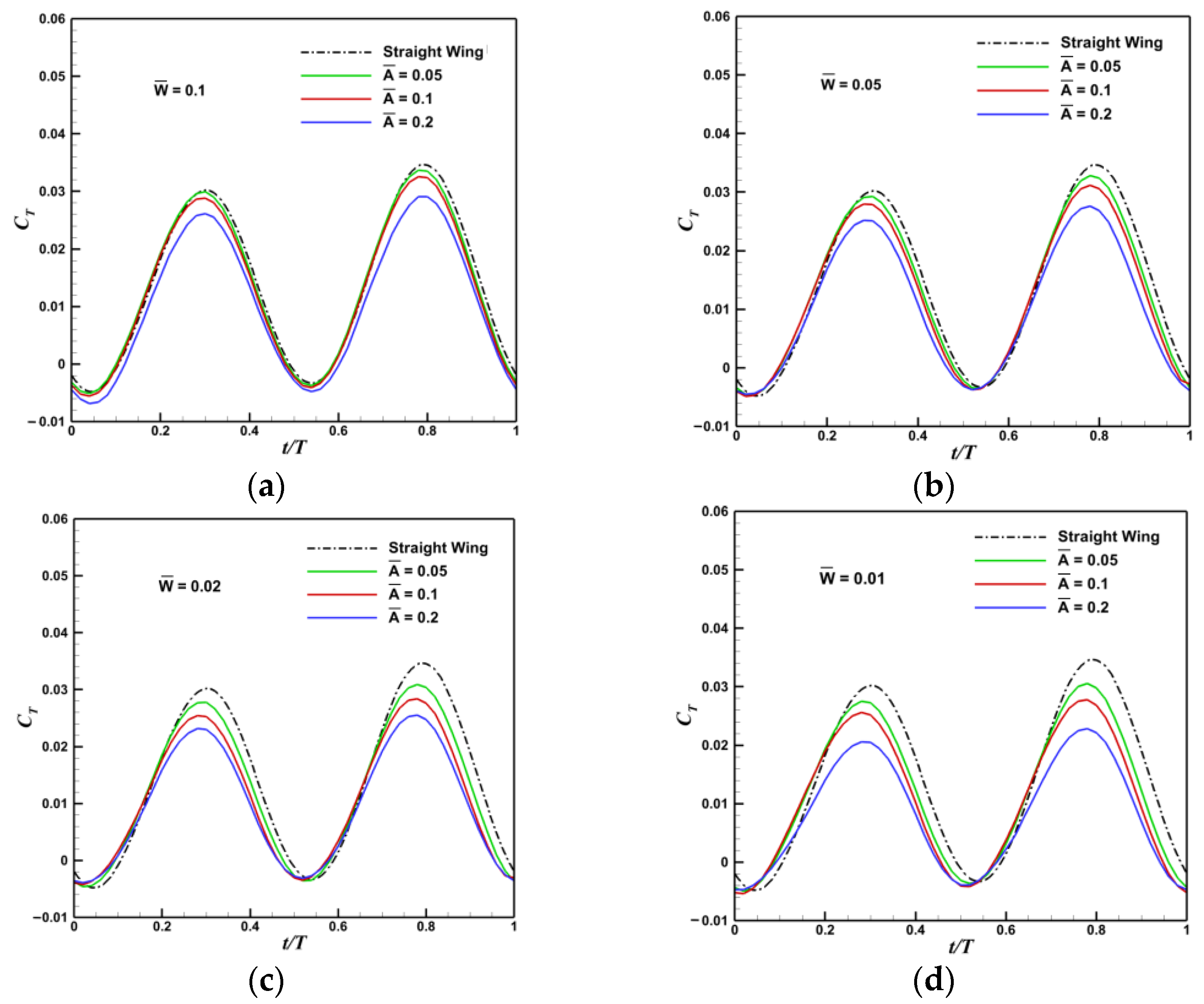
Figure 19.
Time history of trust coefficient in a flapping cycle. (a) ; (b) ; (c) .
Figure 19.
Time history of trust coefficient in a flapping cycle. (a) ; (b) ; (c) .
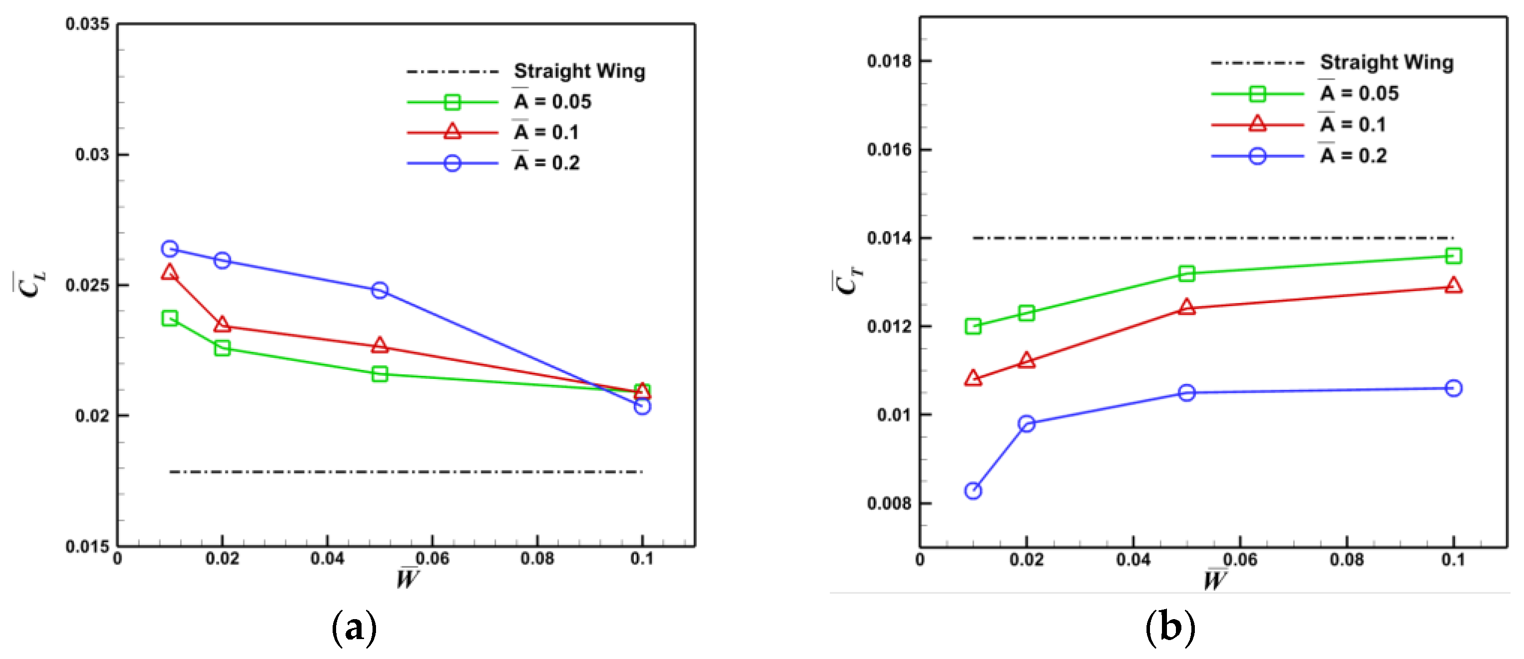
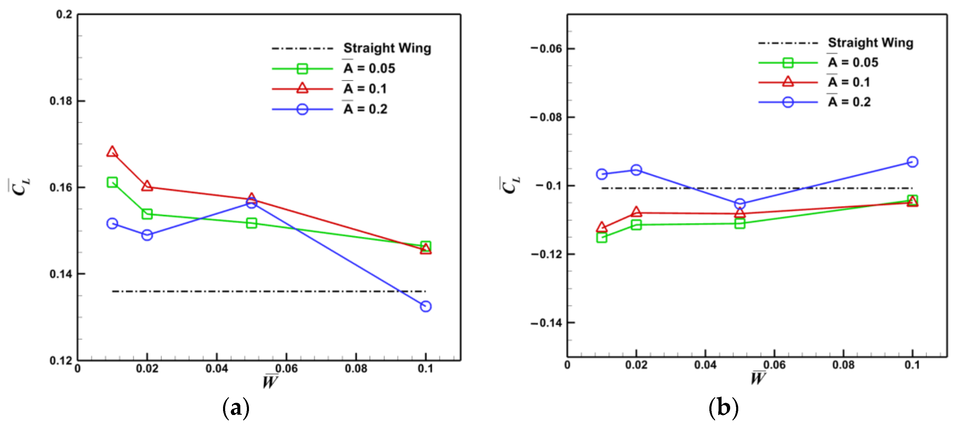
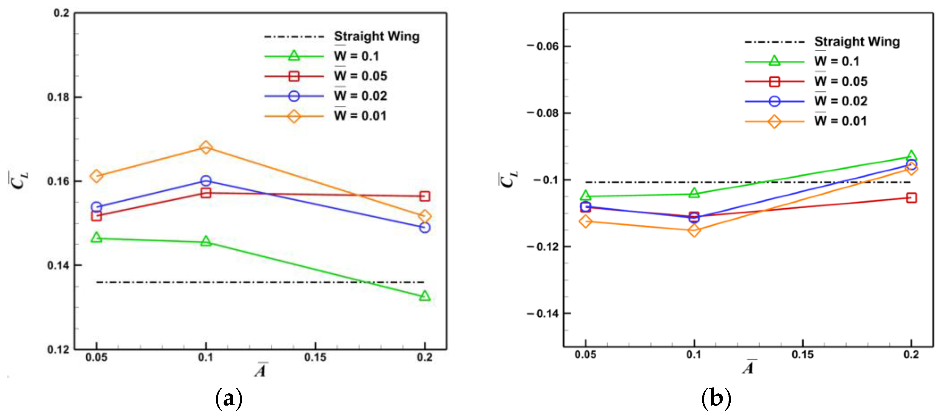
Figure 20.
Comparison of average lift coefficient and thrust coefficient. (a) Time averaged lift coefficient; (b) Time averaged trust coefficient.
Figure 20.
Comparison of average lift coefficient and thrust coefficient. (a) Time averaged lift coefficient; (b) Time averaged trust coefficient.
Figure 21.
Comparison of average lift coefficient of downstroke and upstroke. (a) Time averaged lift coefficient of downstroke; (b) Time averaged lift coefficient of upstroke.
Figure 21.
Comparison of average lift coefficient of downstroke and upstroke. (a) Time averaged lift coefficient of downstroke; (b) Time averaged lift coefficient of upstroke.
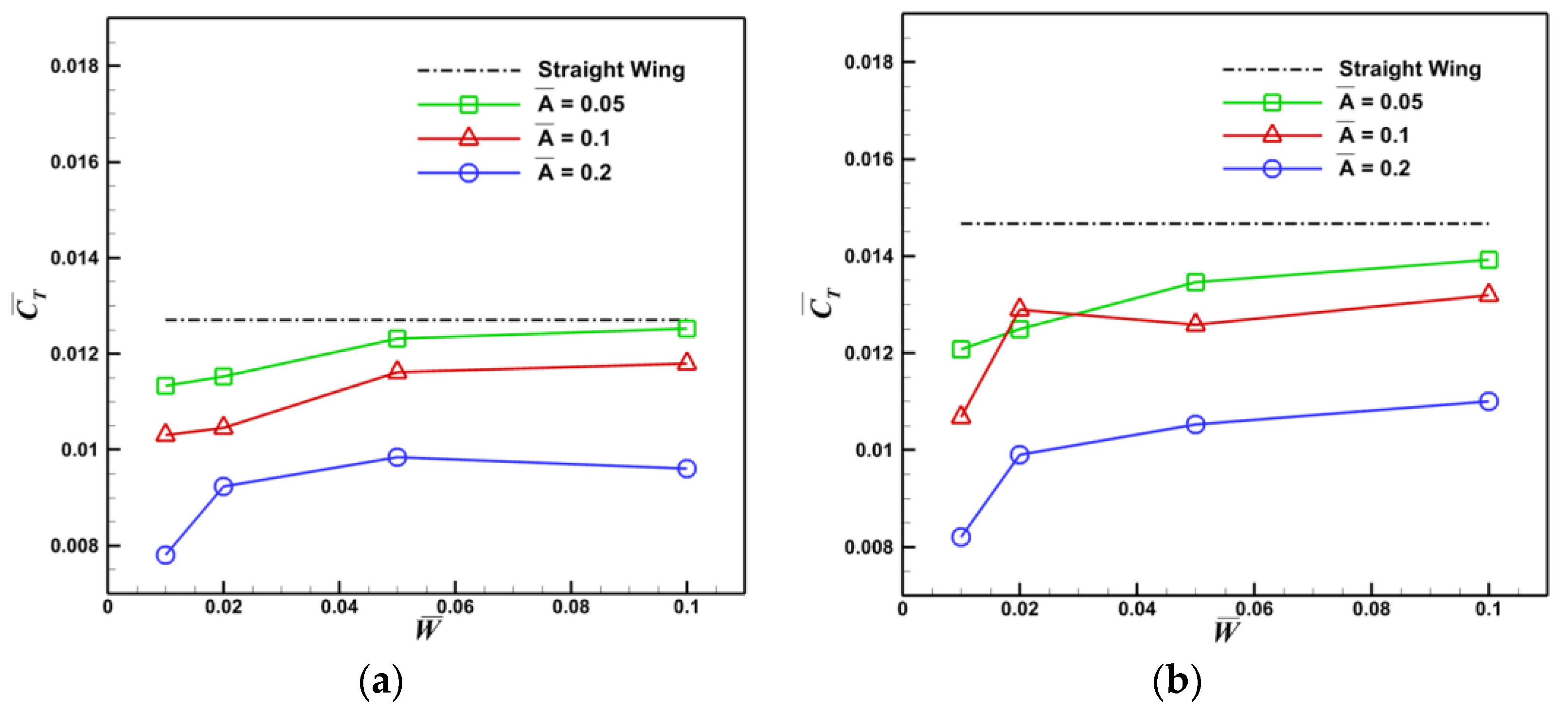
Figure 22.
Comparison of average thrust coefficient of downstroke and upstroke. (a) Time averaged trust coefficient of downstroke; (b) Time averaged trust coefficient of upstroke.
Figure 22.
Comparison of average thrust coefficient of downstroke and upstroke. (a) Time averaged trust coefficient of downstroke; (b) Time averaged trust coefficient of upstroke.
Figure 23.
Pressure contours of the upper surface of flapping wing (Pa). (a) t/T = 0; (b) t/T = 0.2; (c) t/T = 0.5; (d) t/T = 0.8.
Figure 23.
Pressure contours of the upper surface of flapping wing (Pa). (a) t/T = 0; (b) t/T = 0.2; (c) t/T = 0.5; (d) t/T = 0.8.
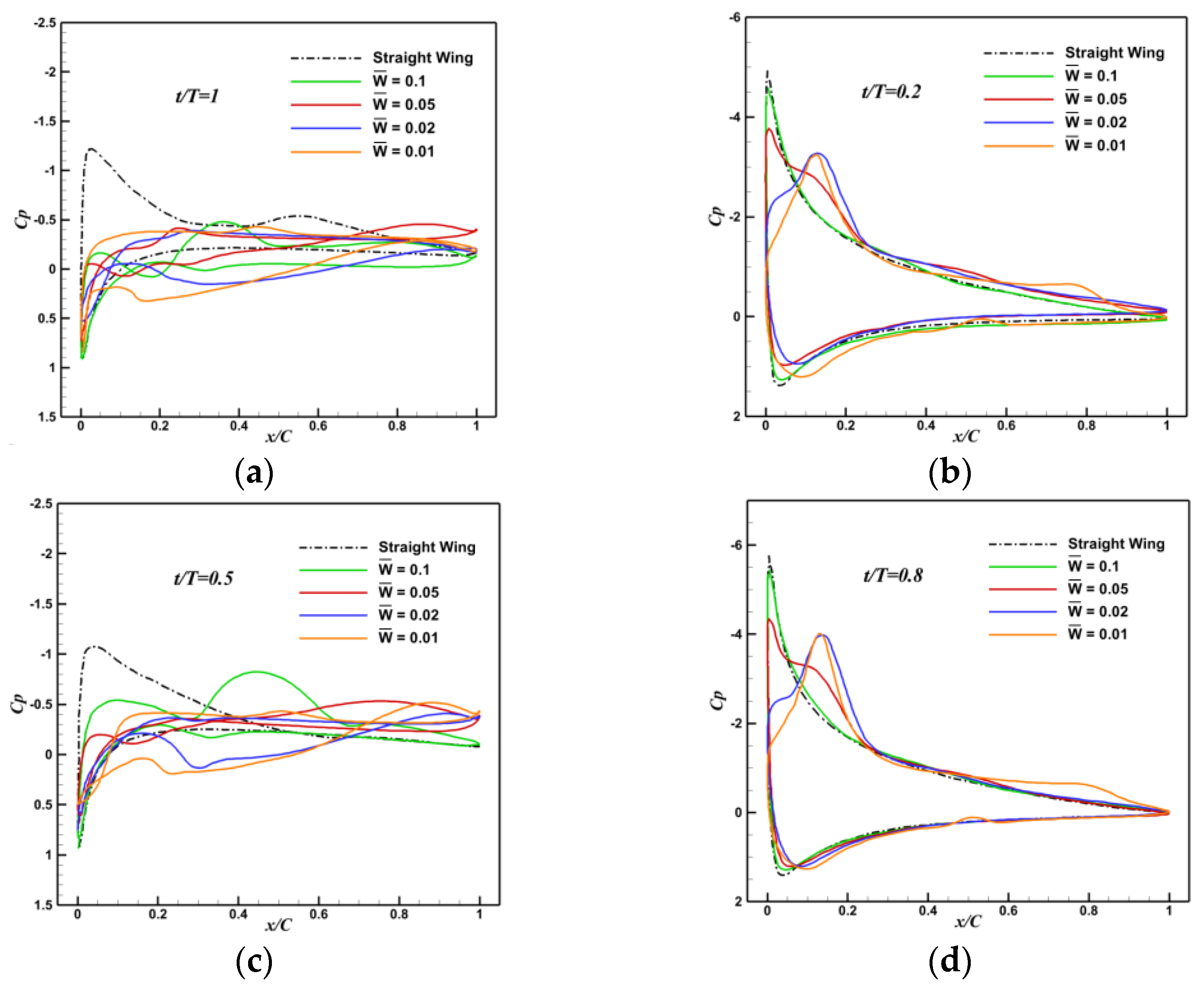
Figure 24.
Pressure coefficient of 80% wingspan section. (a) t/T = 1; (b) t/T = 0.2; (c) t/T = 0.5; (d) t/T = 0.8.
Figure 24.
Pressure coefficient of 80% wingspan section. (a) t/T = 1; (b) t/T = 0.2; (c) t/T = 0.5; (d) t/T = 0.8.
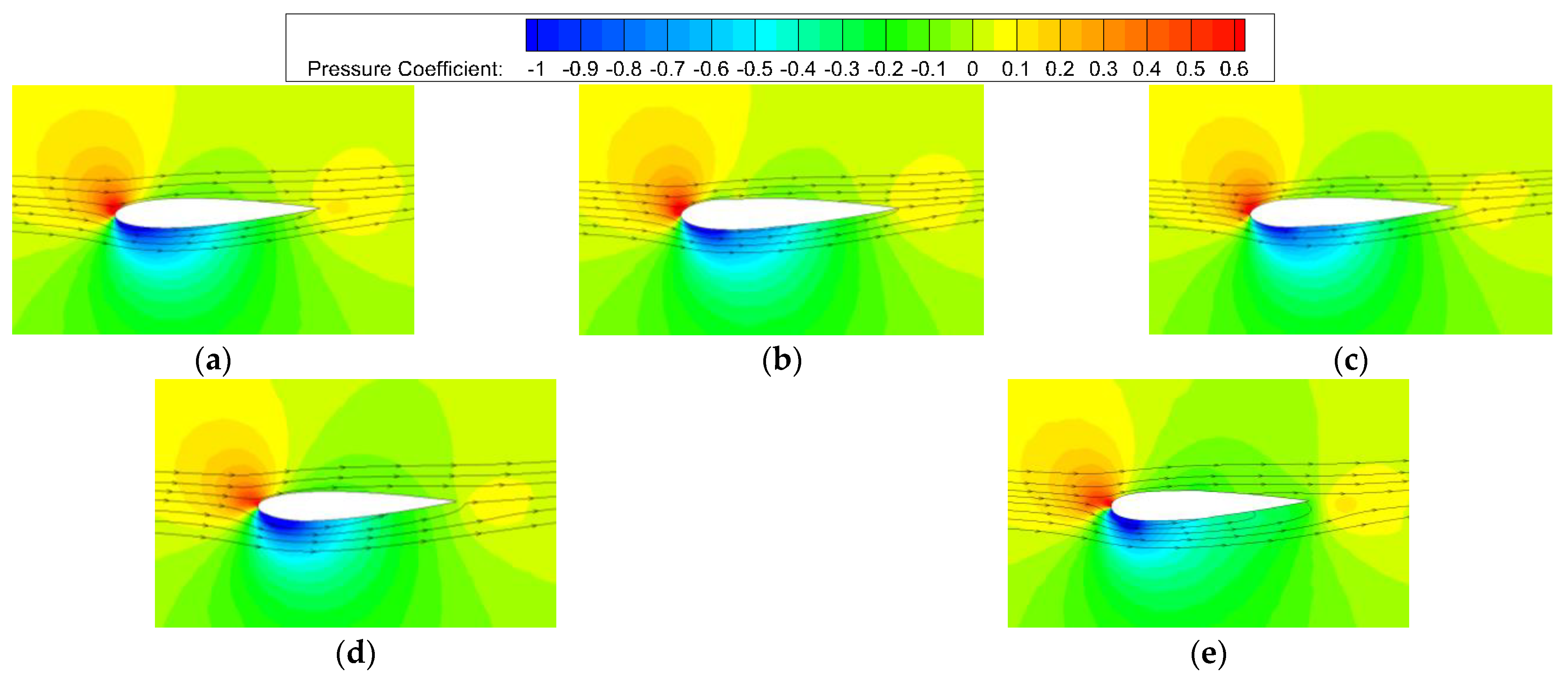
Figure 25.
Pressure contours and streamlines of 50% spanwise section of flapping wing at t/T = 0. (a)Straight Wing; (b) ; (c) ; (d) ; (e) .
Figure 25.
Pressure contours and streamlines of 50% spanwise section of flapping wing at t/T = 0. (a)Straight Wing; (b) ; (c) ; (d) ; (e) .
Figure 26.
Time history of lift coefficient in a flapping cycle. (a) ; (b) ; (c) ; (d) .
Figure 26.
Time history of lift coefficient in a flapping cycle. (a) ; (b) ; (c) ; (d) .
Figure 27.
Time history of trust coefficient in a flapping cycle. (a) ; (b) ; (c) ; (d) .
Figure 27.
Time history of trust coefficient in a flapping cycle. (a) ; (b) ; (c) ; (d) .
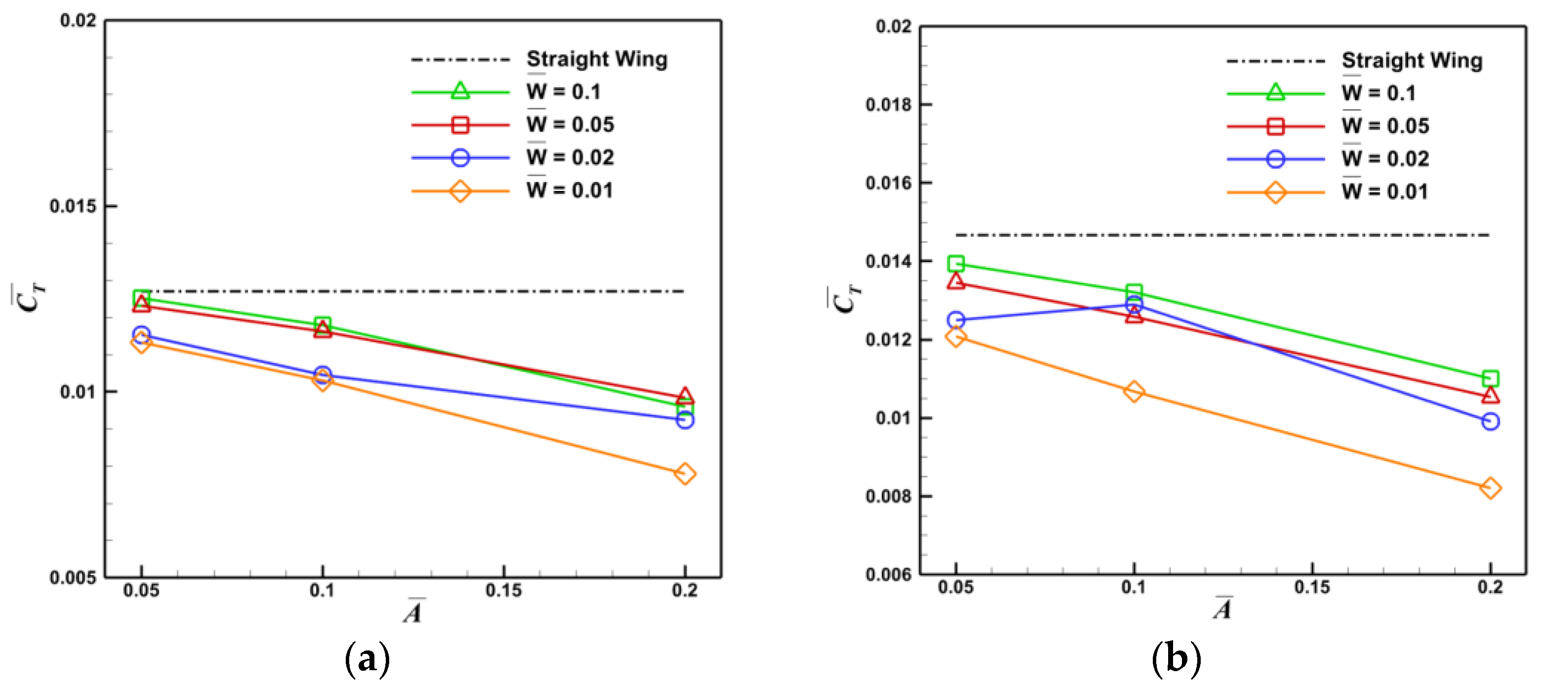
Figure 28.
Comparison of average lift coefficient and thrust coefficient. (a) Time averaged lift coefficient; (b) Time averaged trust coefficient.
Figure 28.
Comparison of average lift coefficient and thrust coefficient. (a) Time averaged lift coefficient; (b) Time averaged trust coefficient.
Figure 29.
Comparison of average lift coefficient of downstroke and upstroke. (a)Time averaged lift coefficient of downstroke; (b) Time averaged lift coefficient of upstroke.
Figure 29.
Comparison of average lift coefficient of downstroke and upstroke. (a)Time averaged lift coefficient of downstroke; (b) Time averaged lift coefficient of upstroke.
Figure 30.
Comparison of average thrust coefficient of downstroke and upstroke. (a) Time averaged trust coefficient of downstroke; (b) Time averaged trust coefficient of upstroke.
Figure 30.
Comparison of average thrust coefficient of downstroke and upstroke. (a) Time averaged trust coefficient of downstroke; (b) Time averaged trust coefficient of upstroke.
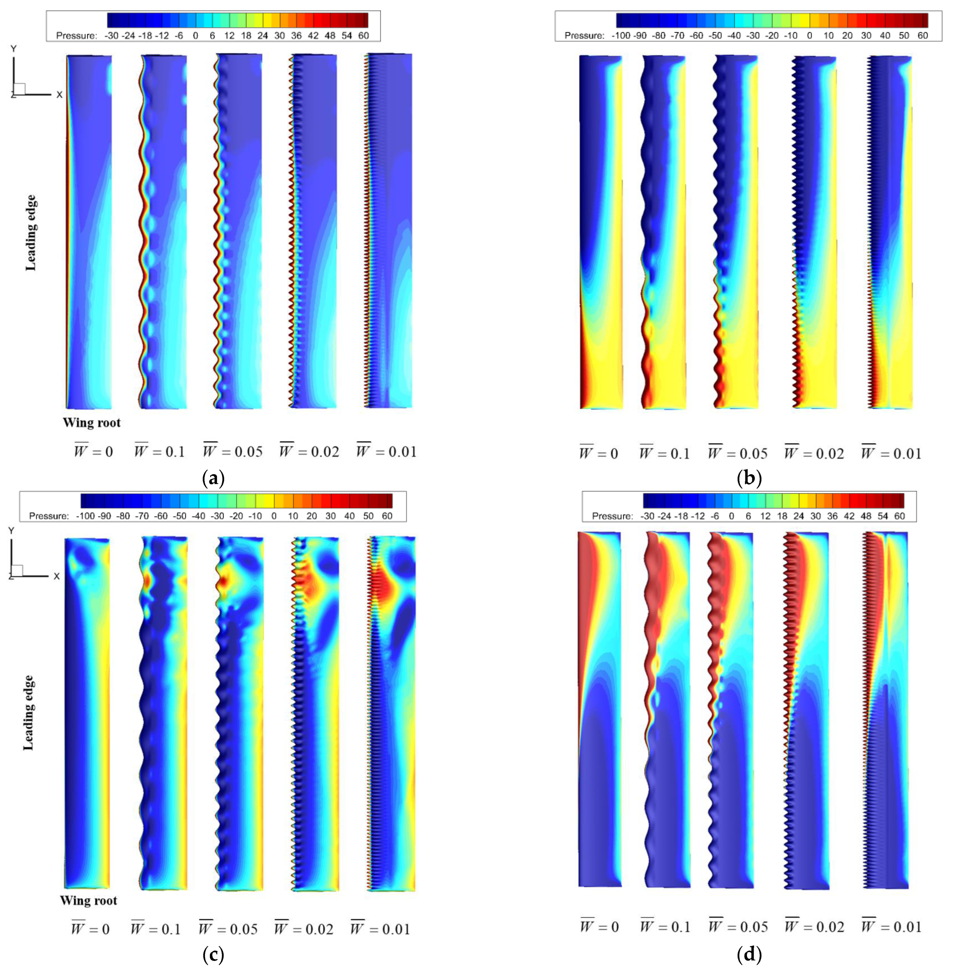
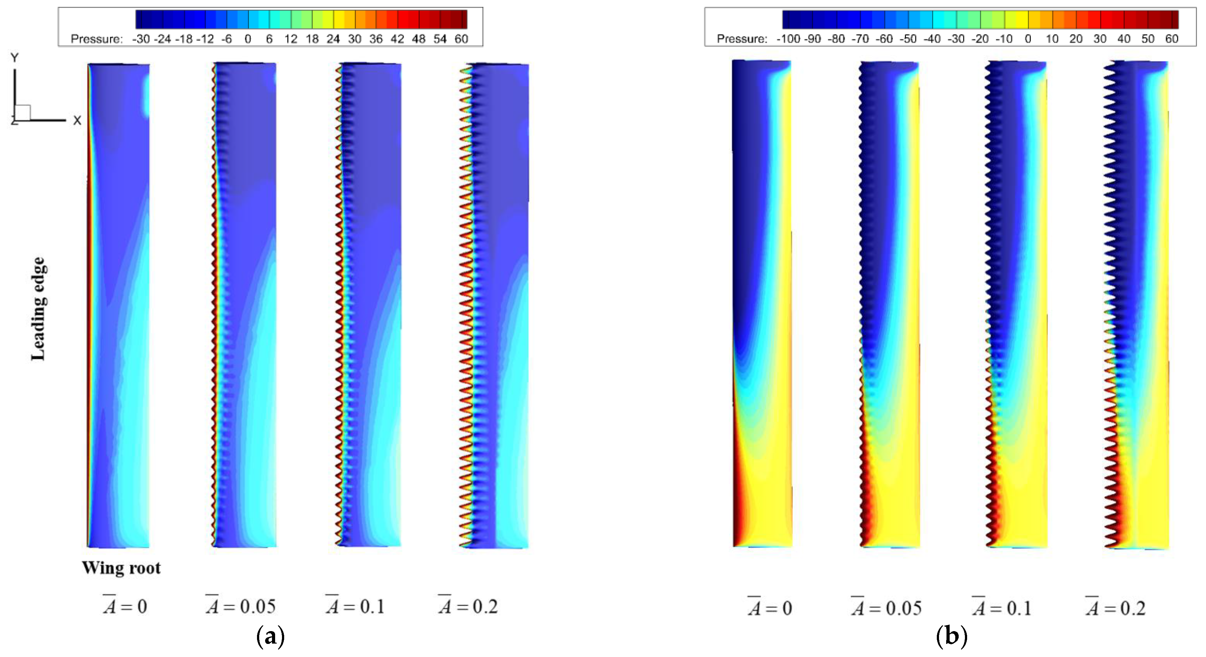
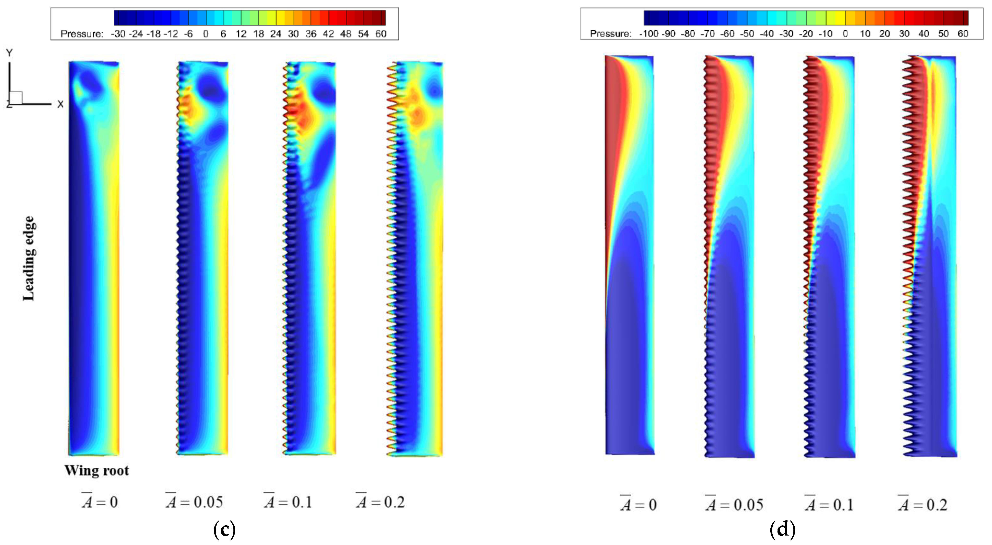
Figure 31.
Pressure contours of the upper surface of flapping wing. (a) t/T=0; (b) t/T = 0.2; (c) t/T = 0.5; (d) t/T = 0.8.
Figure 31.
Pressure contours of the upper surface of flapping wing. (a) t/T=0; (b) t/T = 0.2; (c) t/T = 0.5; (d) t/T = 0.8.
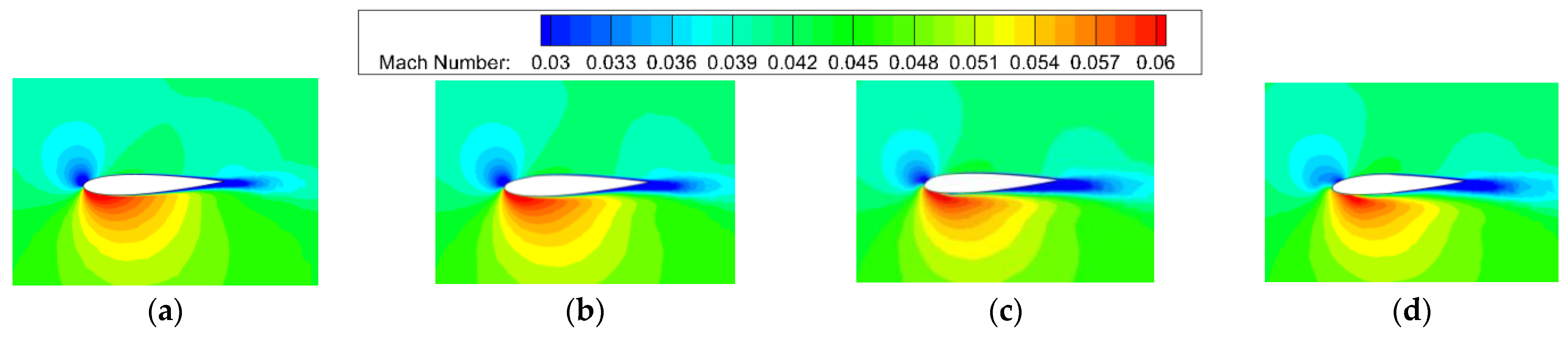
Figure 32.
Mach number contours of 50% spanwise section of flapping wing at t/T = 0. (a) Straight Wing; (b) ; (c) ; (d) .
Figure 32.
Mach number contours of 50% spanwise section of flapping wing at t/T = 0. (a) Straight Wing; (b) ; (c) ; (d) .
Table 1.
Studies on flow control using bionic wavy leading edge.
Table 1.
Studies on flow control using bionic wavy leading edge.
| Author | Object | Method | Reynolds Number | Aerodynamic Performance Change |
|---|
| Fish et al. [11] | NACA63 | Experiment | | The stall angle of attack is delayed by more than 5°. |
| Sudhakar et al. [12] | A high aspect-ratio UAV | Experiment |
| The lift-drag ratio is increased by up to 25%. |
| Sudhakar et al. [13] | NACA 4415 | Experiment | | The separation bubble on the upper wing surface is obviously reduced. |
| Wei et al. [14] | Swept conical SD7032 wing | Experiment | | The stall attack angle is delayed by 2–4 degrees. |
| Abdelrahman et al. [15] | S1223 | Simulation |
| No considerable difference occurs in lift and drag before the stall. |
| Seyhan et al. [16] | NACA 0015 | Experiment | | Lift coefficients have increased by at least 26.2% after stall angles. |
| Gopinathan et al. [17] | NACA 0015NACA 4415 | Experiment/Simulation | | The t/c ratio of the HW flipper is strategically reduced to 0.15. |
| Torró et al. [18] | NACA0021 | Simulation | | The lift coefficient increased by 0.064 and the drag coefficient decreased by 0.045. |
| Ikeda et al. [19] | Serrated single-feather wing | Experiment |
| The lift and lift-to-drag ratio decrease at AoAs < 15°, and the aerodynamic performance of the two is basically the same at AoAs > 15°. |
| Ramachandiran et al. [20] | NACA 0015NACA 4415 | Simulation | | The lift increases at the angle of attack of 11–15 degrees, and the stall angle of attack is delayed by about three degrees. |
| Rostamzadeh et al. [30] | NACA 0021 | Simulation |
| The lift loss is delayed at 18–25° angle of attack. |
| Anwar et al. [33] | insect-like flapping wing | Simulation | 400 | The lift-drag ratio is reduced by 0.34%. |
Table 2.
Relevant parameters of flapping wing.
Table 2.
Relevant parameters of flapping wing.
| Parameter | Value | Parameter | Value |
|---|
| Reynolds number Re | | | 15 |
| 0.12 | | |
| Wing aspect ratio AR | 8 | | 15 |
| 15 | | 0 |
| Mach number Ma | 0.0435 | | 0.25c |
| 8 | | 90 |
| Reduced frequency k | 0.2 | | |
Table 3.
Grid independence verification.
Table 3.
Grid independence verification.
| Case | Number of Background Grid (w) | Number of Component Grids (w) | Total Number of Grids (w) | Total Faces (w) | Total Nodes (w) |
|---|
| Case1 | 70 | 562 | 632 | 3612 | 2565 |
| Case2 | 135 | 706 | 841 | 4554 | 3150 |
| Case3 | 289 | 836 | 1125 | 6908 | 4816 |
Table 4.
Wavy leading edge flapping wing configuration.
Table 4.
Wavy leading edge flapping wing configuration.
| Configuration | | | Configuration | | | Configuration | | |
|---|
| 1-1 | 0.05 | 0.1 | 2-1 | 0.1 | 0.1 | 3-1 | 0.2 | 0.1 |
| 1-2 | 0.05 | 0.05 | 2-2 | 0.1 | 0.05 | 3-2 | 0.2 | 0.05 |
| 1-3 | 0.05 | 0.02 | 2-3 | 0.1 | 0.02 | 3-3 | 0.2 | 0.02 |
| 1-4 | 0.05 | 0.01 | 2-4 | 0.1 | 0.01 | 3-4 | 0.2 | 0.01 |
Table 5.
Average change rates of flapping wings at different wavelengths.
Table 5.
Average change rates of flapping wings at different wavelengths.
| 0.1 | 0.05 | 0.02 | 0.01 |
|---|
| 16.01%↑ | 28.89%↑ | 34.32%↑ | 41.04%↑ |
| 11.66%↓ | 14.04%↓ | 20.71%↓ | 25.97%↓ |
Table 6.
Average change rates of flapping wings at different amplitudes.
Table 6.
Average change rates of flapping wings at different amplitudes.
| 0.05 | 0.1 | 0.2 |
|---|
| 24.34%↑ | 29.33%↑ | 36.52%↑ |
| 8.75%↓ | 15.53%↓ | 29.03%↓ |
Table 7.
Sensitivity of design parameters.
Table 7.
Sensitivity of design parameters.
| | Wavelength | Amplitude |
|---|
| −77.4% | 22.6% |
| 52.9% | −47.1% |


