1. Introduction
Multilink (anthropomorphic) robot manipulators allow you to perform high-precision technological operations. As a rule, they have a degree of mobility of at least six, which allows the manipulator to be positioned in any position within its working space [
1,
2,
3,
4,
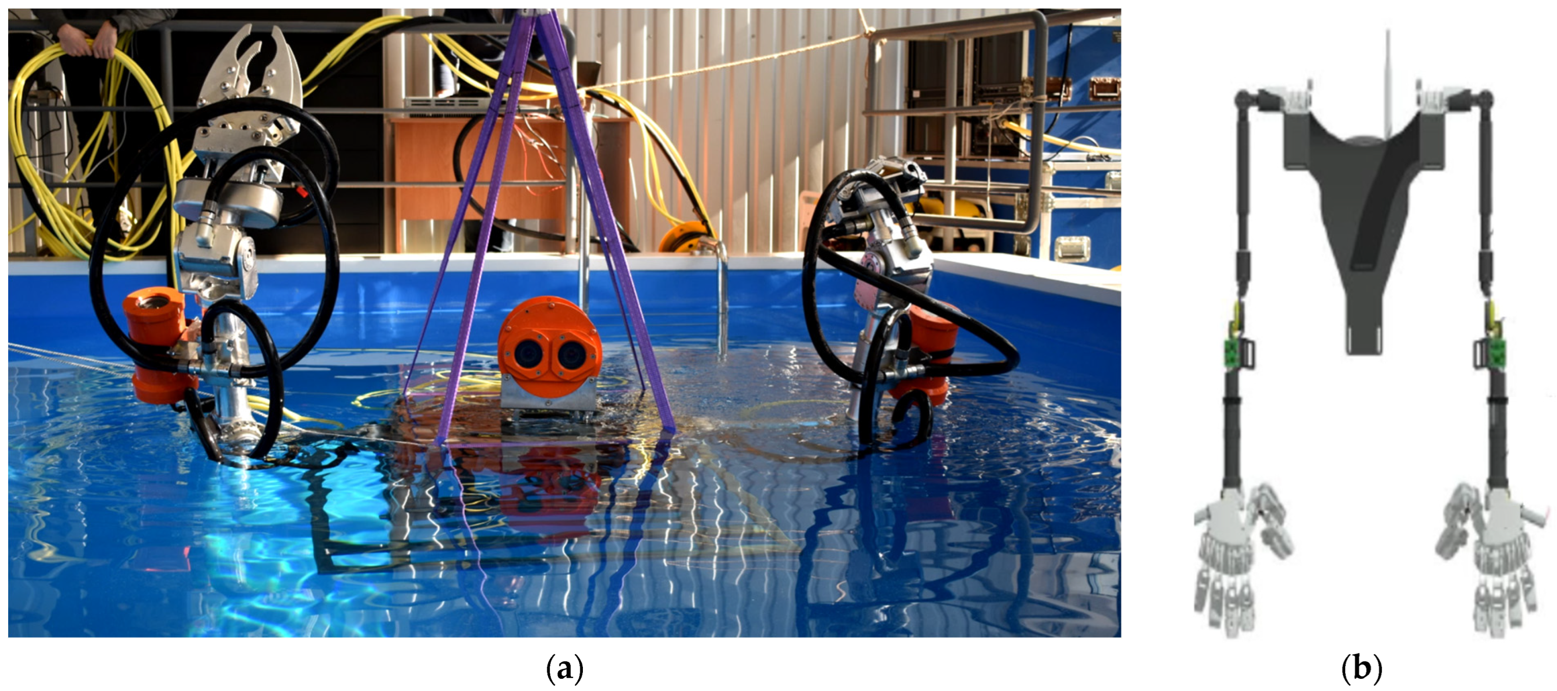
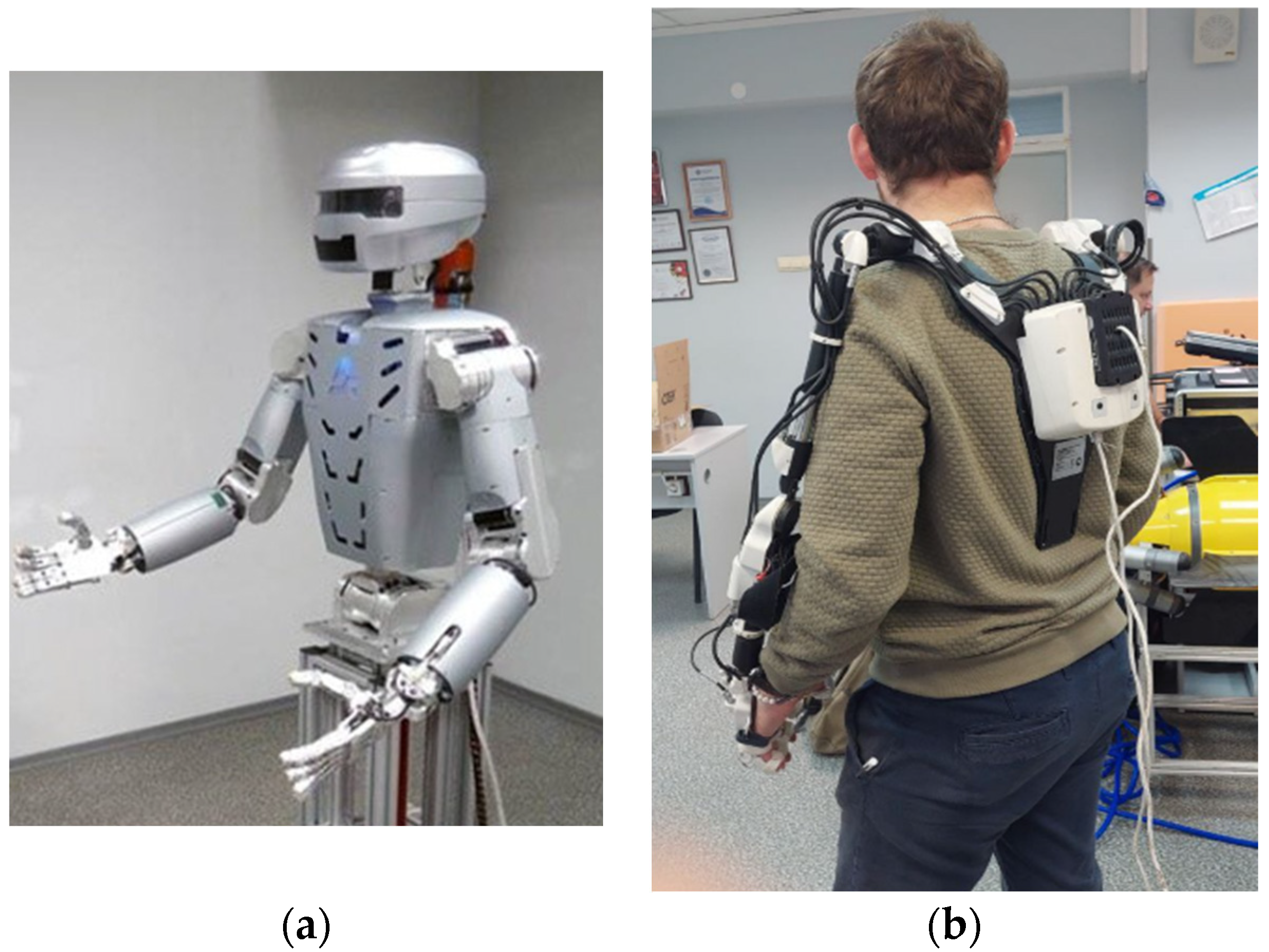
5]. Nowadays, the field of marine robotics application is expanding due to the need to increase the efficiency of many underwater operations (laying and maintenance of underwater communications, underwater construction, search and rescue operations, etc.). To solve these problems, it is necessary to provide a high degree of autonomy of underwater robots with realization of functions of effective and safe manipulation in water environments along complex pro-spatial trajectories. The use of multilink manipulators installed on uninhabited underwater vehicles allows some underwater technological and research operations to be performed. Such manipulators are installed on the robots “Ichtiandr” (
Figure 1) and SAR-401 (
Figure 2) [
6,
7,
8], developed in the company “Android Technics”, Magnitogorsk, Russia.
Speaking about increasing the level of autonomy of underwater manipulation operations, it is necessary to take into account that in addition to positioning robot manipulators in a given point of space in front of the manipulated object, most other tasks are related to ensuring operational functions (e.g., keeping the object in the center of the working area, stabilizing the robot position, etc.) and safe operation of the entire system (avoiding limiting and singular positions of the manipulator, avoiding self-collisions and collisions with other objects). All this leads to the fact that, although the human operator is no longer in an aggressive environment, he is still under severe stress when performing complex manipulation tasks in the underwater environment. In particular, and for this reason, recent research is aimed at increasing the level of autonomy in underwater operations, either by fully automating simple typical actions or by introducing some autonomous control functions for teleoperated ROVs to facilitate and improve the quality of the operator’s work.
An obvious approach to building control of multilink manipulators is the approach based on building a mathematical model of manipulators and solving the inverse kinematics problem (IKP). The mathematical models of robots do not take into account nonlinearities. The different instances of the same robot model may have different mathematical models depending on their wear and calibration. The generalized coordinates of manipulators have different limits. The control of multilink manipulators is complicated by the presence of kinematic limitations in their degrees of mobility, degenerate positions characterized by the ambiguity of the OPC solution, as well as by the limited working zones in which their working tools can approach the objects of work with the given angles of service. Depending on the type of technological operations performed, these working zones for the same manipulators can be different. As a technological operation, we can consider the cutting process, when pneumatic scissors are used as one end-effector of the “Ichtiandr” robot and a gripper is used as the second (
Figure 1).
The nonlinearity of the mapping of the manipulator’s joint space to the Cartesian workspace complicates the direct solution of the IKP [
9]. It becomes more difficult to obtain the solution of the IKP as the number of manipulator links increases and nonlinearities appear. The solution of the IKP for redundant manipulators also requires a complex solution of the pseudo-inverse Jacobi matrix [
10].
The application of conventional numerical methods to solve the IKP requires significant time consumption [
11]. Methods based on the fuzzy logic can be applied to the solution of the IKP [
12,
13]. These methods are not computationally expensive. However, like numerical methods, they do not take into account the possibility of the multilink manipulator entering special positions.
In [
7,
14], the Artificial Neural Networks (ANN) approach to the control of multilink manipulators was proposed. The methods based on the application of the ANN approaches allow unambiguously solving the IKP with a given accuracy and taking into account the constraints on the generalized coordinates of the multilink manipulator having excessive degrees of mobility.
When solving manipulation tasks, including underwater ones, it is often impossible to determine in advance the exact shape of the object of interest, as well as the mutual location of the underwater robot and this object. Then, it is necessary to form the manipulator’s control bypassing the stage of testing. It can lead to self-collisions.
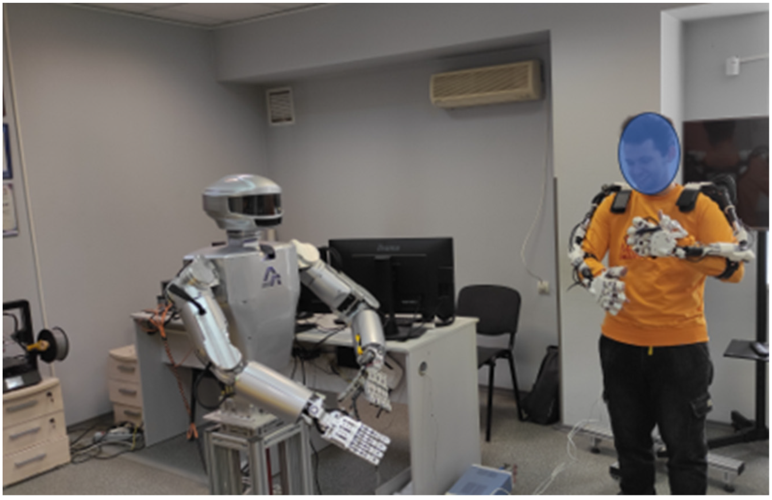
When implementing copying control of manipulators [
14], it is very likely that self-collision of manipulators will occur (
Figure 3).
A number of methods additionally use sensors installed on manipulators [
15,
16]. Sensors are usually implanted directly inside or outside robot arms. An example of such a method is, for example, the “skeleton algorithm” [
17]. This algorithm requires sensory information about the position of each link during movement in order to plan evasive trajectories before possible collisions.
For anthropomorphic manipulators, there is a problem of collision of all its nodes. For example, a collision may occur between the first link of the left manipulator and the penultimate link of the right manipulator. It is not advisable to install sensors on all links and the sensor must monitor the space around it 360 degrees. Sensor methods are expensive and cannot be used in simulation studies [
18].
The most modern collision detection methods are based on analytical approaches [
19,
20,
21,
22,
23,
24,
25,
26]. In [
7], an ANN solution on the basis of the “Contextual” ANN to predicting the self-collision of multilink manipulators is proposed. This method implements a regression approach. The proposed solution results in high accuracy and allows the possibility of self-collision in an online mode to be checked.
From the point of view of the authors, the study of the possibility of the ANN solution based on the classification problem to predict the self-collision of multilink manipulators is interesting. This approach will allow us to give an unambiguous answer to the following question: will there be a self-collision or not? Based on the fact that due to the difficulties in analytically finding the global extremum, the construction of the ANN is often experimental in nature; in this paper, we will present a description of the construction of the ANN by experimentally selecting its parameters to solve the classification problem as a method for predicting self-collision. The main advantages of this method are the high speed of calculations and the ability to use this method without calculating the parameters and dimensions of the robot. This makes it possible to use an ANN approach for manipulators to which there is no physical access and, accordingly, it is impossible to calculate the inverse kinematics problem. The ANN proposed in this paper characterizes the position of manipulators in space and classifies the state of their location.
The rest of this paper is organized as follows. Description of the class of systems and the problem statement are presented in
Section 2.
Section 3 introduces the ANN training parameters. At the same time, we provide the development of the ANN in
Section 4. Finally, we summarize the contributions of our work and discussion in
Section 5.
2. The Description of the Robot: The Formulation of the Problem
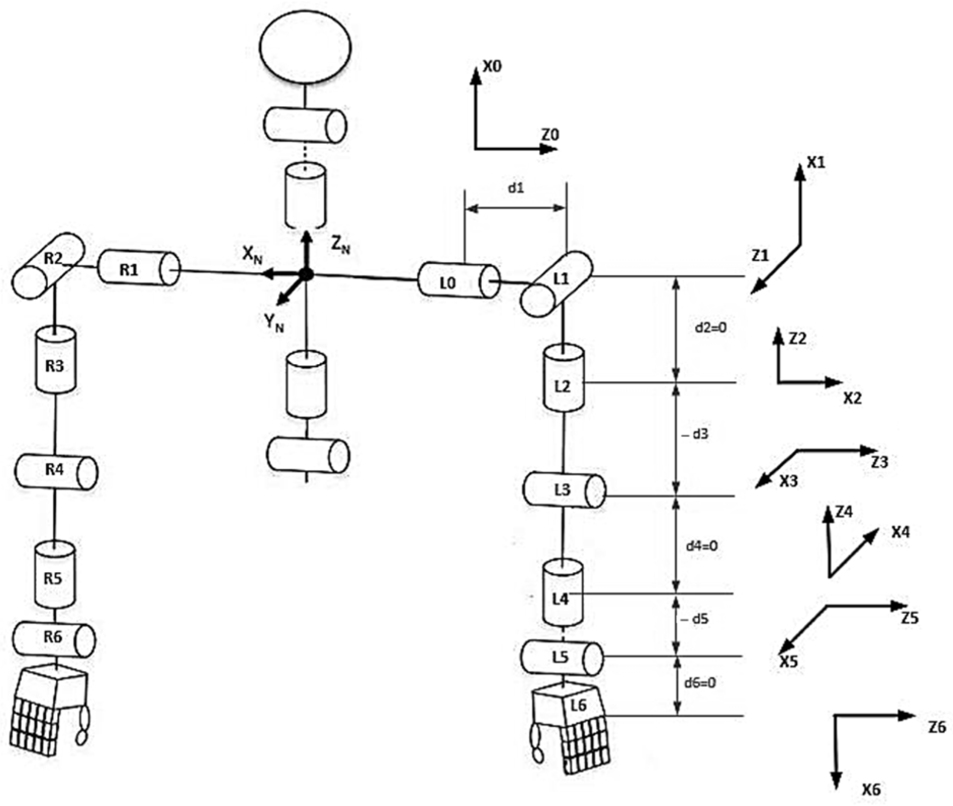
2.1. The Kinematic Scheme of the Manipulator
As stated in [
7,
14], the manipulators of “Ichthiandr” or SAR-401 are considered. Let us briefly repeat the description of the manipulator geometry using Denavit–Hartenberg (DH) notation and methodology [
27] (the parameters of the manipulator are given in
Table 1 and
Table 2) and the kinematic diagram (
Figure 4).
, , , —the DH parameters. For the right manipulator, the DH parameters are identical.
The initial coordinate system associated with the first joint is
. The final coordinate system associated with the manipulator end-effector is
. The extended position vectors are
and
where
—the matrix of homogeneous transformation.
For each joint, we can define a homogeneous transformation matrix . To generate an output sample for training the ANN, we will compose six transformation matrices for the manipulator links, with the help of which the input data for training the ANN will be generated , , , , , .
2.2. The Classification Task
Let us give a description of the construction of the ANN for the problem of detecting of the manipulators self-collision based on solving the classification problem.
Classification solves the following problem. There are two types of classes consisting of values: collision detection and collision absence. There is a set of manipulator positions for which it is known to which class they belong. This set of positions is the training sample. The belonging of other random states of manipulators is not known. It is required to build an algorithm capable of classifying arbitrary manipulator positions.
Since there are very few significant events in the network training sample, a study is conducted to train the ANN in binary classification and multiclass classification tasks.
The ANN training in binary classification tasks is performed on a set of training examples for which the object belonging to class A or class C is known. As class A, we will understand the collision state (provided that collision between manipulators is detected), and class C is the state in which there is no collision. Class A is assigned.
The formal formulation of the two-class collision classification problem is as follows:
where
—training samples,
—set of permissible values of the trait.
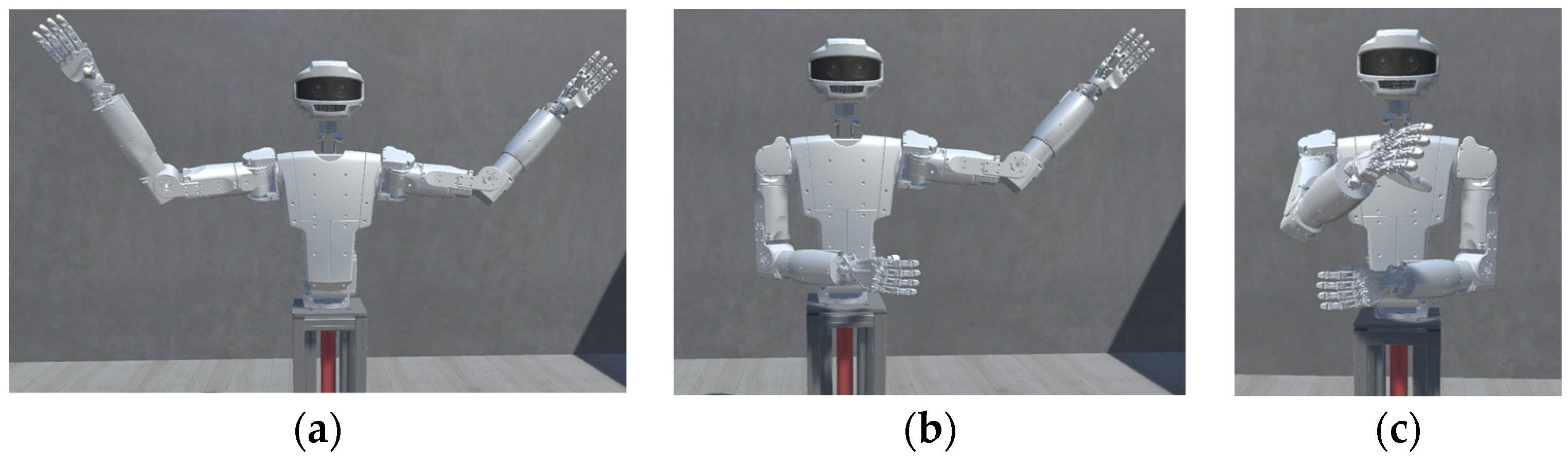
To solve the classification problem with three classes, multiclass classification is used as the classes of which three states were used: collision, threat of collision, and no collision:
where as before, class A—collision condition, class C—absence of collision, and class B—threat of collision. Class B is assigned when one or two manipulators are in the collision zone, but no collision has occurred. In the process of training, we will denote the belonging to classes: class A—Collide, class C—Out, class B—Warning. The external state of the classes is shown in
Figure 5 and
Figure 6.
3. ANN Training Parameters
3.1. The Input Data
At the initial stage of the ANN design, the dataset on which the network will be trained is prepared. Since coordinates in space and end-effector rotation position are mainly used in robot control, it is necessary to know at which positions of two manipulators at certain coordinates a collision will occur.
Taking into account the choice made in [
7,
14], we will feed to the input of the ANN elements of the transformation matrix.
As a result, a vector
is the input of the ANN.
As classified observations, we use collision information, which is distributed as above in the case of using binary classification into two classes, presence and absence of collision, and in the case of using multiclass classification into three classes, presence, absence, and possible collision (threat of collision).
Collection of training data consists in random positioning of manipulators by the operator, for example, with the help of a copying suit, and obtaining by means of a direct kinematics problem from the robotics complex for each manipulator position a transformation matrix and fixing the current state on the presence of a collision or not. In order to obtain training data for the ANN, let us compose the configuration space of the robot as a set of its possible configurations.
To prepare training data, we will randomly select possible positions of the robot servos in different places of its working area. The obtained data will be stored in the form of vectors of left and right manipulator positions, respectively (6):
where
is the servo rotation angle of the
i-th joint.
By solving the direct kinematics problem, we obtain two transformation matrices for the left and right manipulator (5), using the values of which we will form the input dataset (4). We will use binary or multiclass classification as output.
The input parameters characterizing the position in space of each manipulator are given in
Table 3.
Table 3 shows examples of 13 observations. The first 12 rows of the table contain the values of the transformation matrix of the left manipulator. Rows 13 through 24 contain the values of the right manipulator transformation matrix. The last row contains the output parameter of the classification.
3.2. The Activation Function of the Output Layer
Since the research uses samples with binary and multiclass classification, we will use the softmax function—a logistic function for the multivariate case, as the activation function. This will allow us to preserve the network structure and conduct comparative analysis on identical networks. Also, the use of softmax will ensure compatibility in case of changing the number of classes.
The softmax function is applied to a vector rather than to a single value. For multiclass classification, the ANN is built in such a way that the number of neurons on the last layer is equal to the number of classes to be searched. In this case, each neuron should produce a value of the probability of the object belonging to the class, i.e., a value between zero and one, and the sum of all values should give one. When performing multiclass classification using the softmax function, the limitation is that the model predicts only one class among all classes. In other words, the values in the vector represent the probability of a class occurring. The sum of the probabilities will be equal to 1. The larger probability value will determine the class.
The mathematical description of softmax function has the form
where K indicates the number of classes.
3.3. Quality Measures of Classifiers
To construct the confusion matrix, we will consider the following quality measures of classifiers for binary classes.
Accuracy—fraction of correct answers of the algorithm
where TP (True Positive) is the number of correctly predicted positive values; TN (True Negative) is the number of correctly predicted negative values (the result and prediction are negative; the prediction coincided with reality); FP (False Positive) is the number of incorrectly predicted negative values (the model predicted a positive result, but in fact it is negative); FN (False Negative) is the number of incorrectly predicted negative values (the model predicted a negative result, but in fact it is positive). Note that this metric does not work in tasks with unequal classes.
The denominator of Formula (9) is the number of positive (correct) values predicted by the classifier. The closer the Precision value approaches 1, the higher the accuracy.
The denominator of Formula (10) is the number of positive responses in the data, reflecting how many true outcomes were predicted correctly. The closer the Recall value approaches 1, the higher the coverage of correct solutions. The ideal classification solution occurs when Precision and Recall are equal to 1.
Error (prediction error). This measure is expressed as the ratio of all errors made to the total number of significant events, namely the number of collisions involved in training.
where AllCollide is the total number of collisions in the sample. Under ideal conditions, Formula (11) should tend to 0.
Using the above quality measures of the classifiers, a confusion matrix is generated for clarity.
3.4. The Training Method
The holdout validation method is chosen as the network training method, which is recommended for use in large datasets as opposed to the cross-validation training method, which uses the same data points for training and testing. In the cross-validation method, the data are divided into k equal subsets. Training takes place k times such that each of the k subsets is used as a test set, and the other subsets are combined to form the training set. Then, the results of each training iteration are added up and the average value is found to obtain the generalized efficiency of the model. According to the research conducted, using cross validation leads to overfitting when solving the problem. According to the results of training, we obtain 100% accuracy on the training sample, but when testing the network on another random sample, the collision prediction error grows up to 5%. Such scatter in accuracy indicates that the network is overfitted.
4. The ANN Design
A number of the ANN variants were considered for research to select the network architecture. We will present the characteristics of the most significant ANN obtained during the design process.
4.1. Simple ANN with Binary Classification
Network 1 is simple feed forward ANN. The parameters of Network 1 are given in
Table 4.
The rules for determining the dimension of the hidden layer are defined in [
28,
29,
30].
As a variant of the network realization, we can consider using the Matlab 2023a fitcnet function. We prepare two datasets of different sizes (
Table 5) as input data. Hereinafter, the dataset is built based on the possibilities of the experiment.
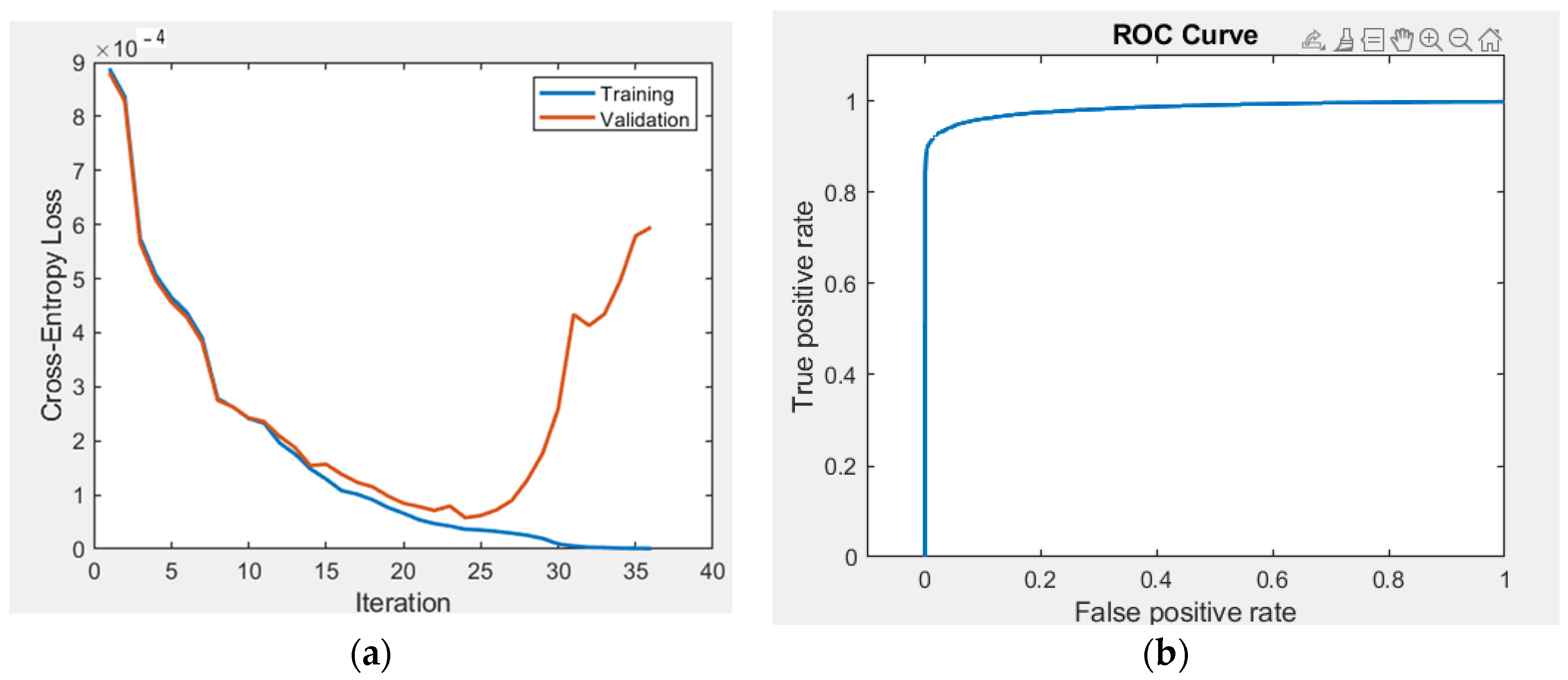
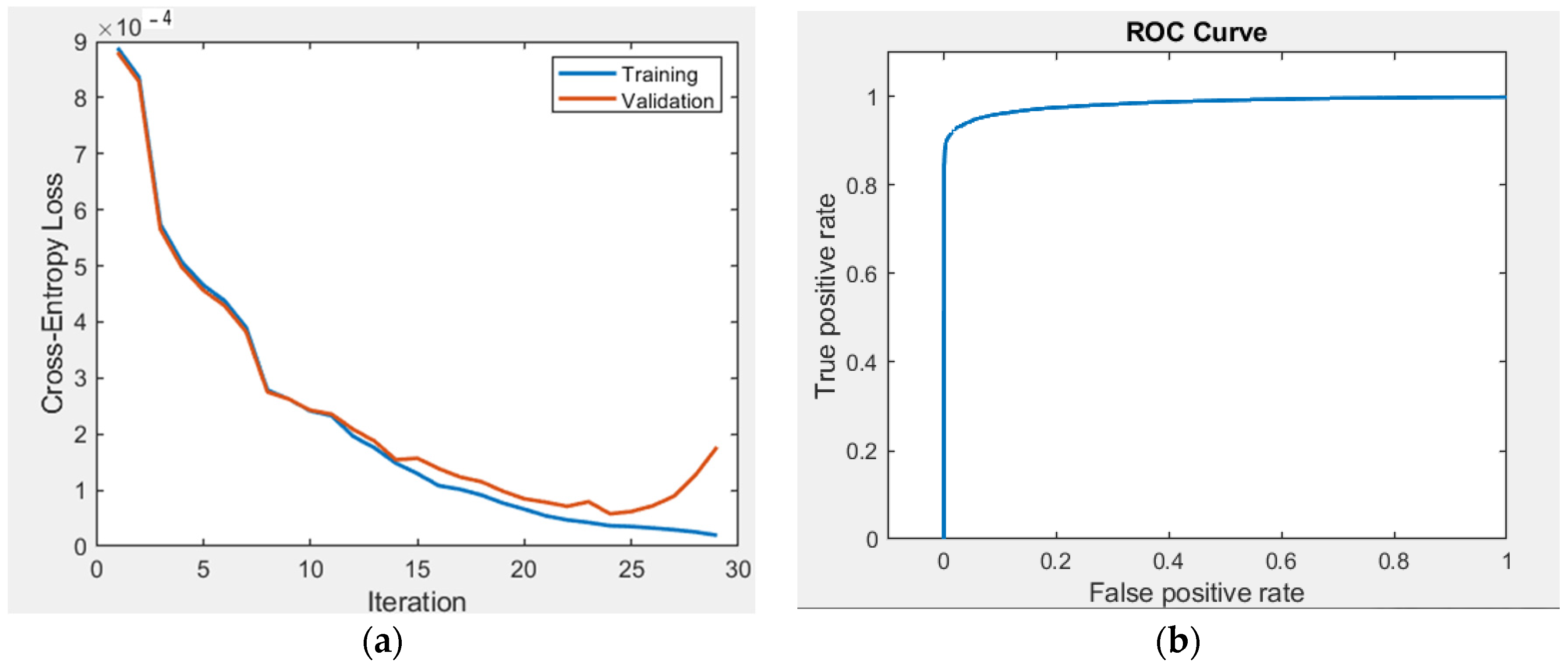
At first, we will use Dataset 1. The results of training Dataset 1 on the raw sample are shown in
Figure 7.
From
Figure 8, we can see that the training ended at 25 iterations. Since we use a large number of input parameters (24 values), 25 iterations are not enough to train the network and the number of iterations should be larger.
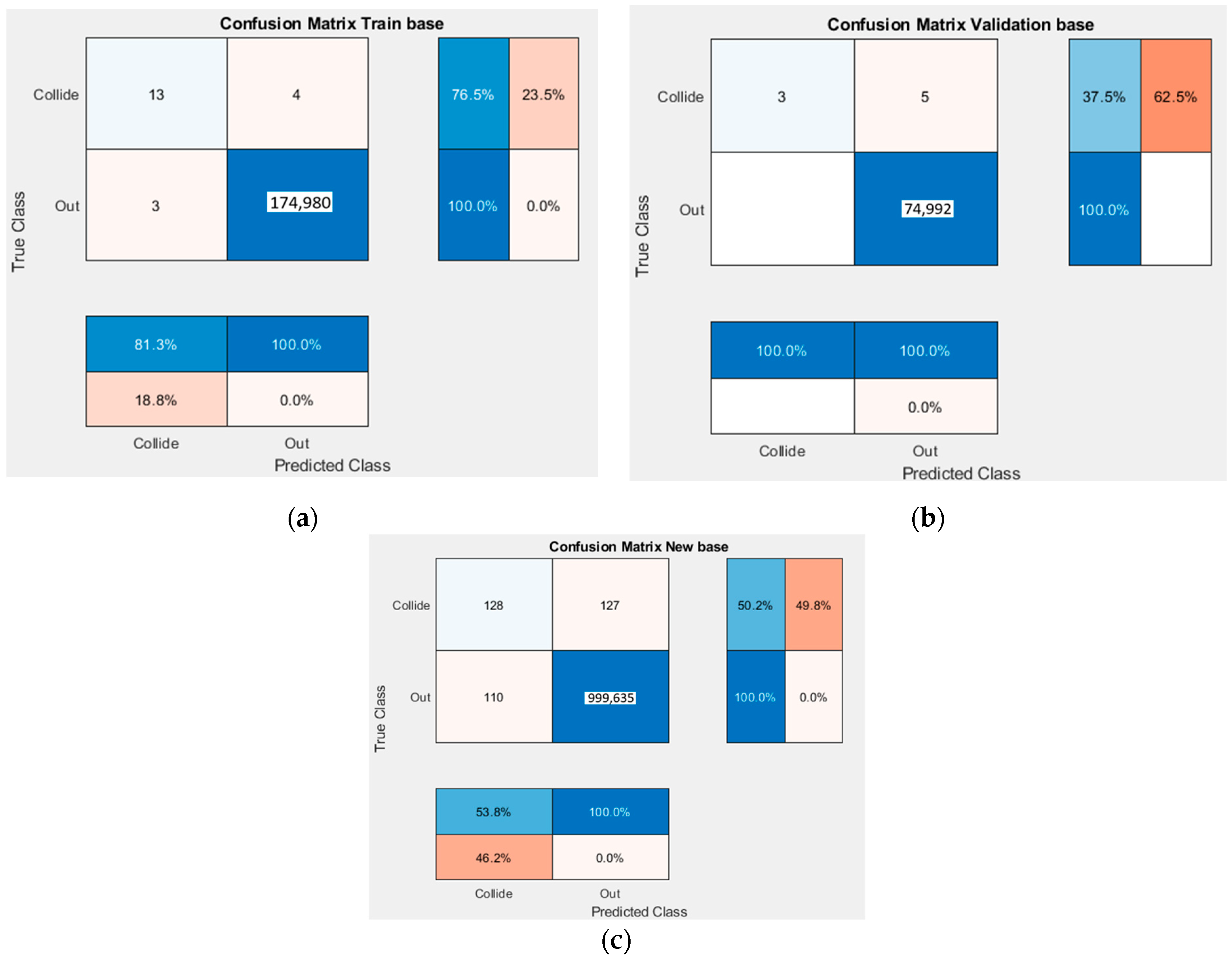
Also, to evaluate the solution, we run the trained network on three validation bases: a sample of data on which training was performed, a sample of data that was selected as a validation sample from the total dataset constructed for training, and a sample of random data designed to validate the trained network on values that were not considered during training. The results obtained are summarized in
Table 6. The confusion matrices obtained from the results of the network are shown in
Figure 8.
The obtained accuracy is too high, which does not correspond to reality. This is due to the fact that the number of significant events in Dataset 1 does not exceed 0.01% of all values in the sample. Determining the accuracy of network training over the entire dataset will not give an accurate representation of the correctness of network training, since significant events border on the margin of error. Calculated solution accuracy against the entire dataset will give an overestimated accuracy. The accuracy metric does not work in tasks with unequal classes.
Hereinafter we will use Precision, Recall, Error criteria to determine accuracy. The results obtained are summarized in
Table 7.
As a criterion for evaluating the accuracy of the network, we will use prediction error as the ratio of the sum of all errors to the total number of items in the dataset (Formula (12)), since it is important that the network makes prediction errors as rarely as possible. Dataset 1 performs poorly. There were problems with both bias and spread. The accuracy of the solution is not satisfactory for the task.
Consider Network 2, which differs from Network 1 by the number of neurons equal to 47. The choice of the number of neurons is conditioned by the rule for the hidden layer configuration [
28,
29,
30]. The results of training the network are shown in
Figure 9. The collision detection accuracy obtained from the training results is presented in
Table 8.
Even though the accuracy of the solution on a random sample is higher, it is still not satisfactory for the problem at hand.
Consider Network 2, increasing the number of elements in the training sample with the help of the prepared Dataset 2 (
Table 4), assuming that there may not be enough significant values in the training sample. We will call this network—Network 3.
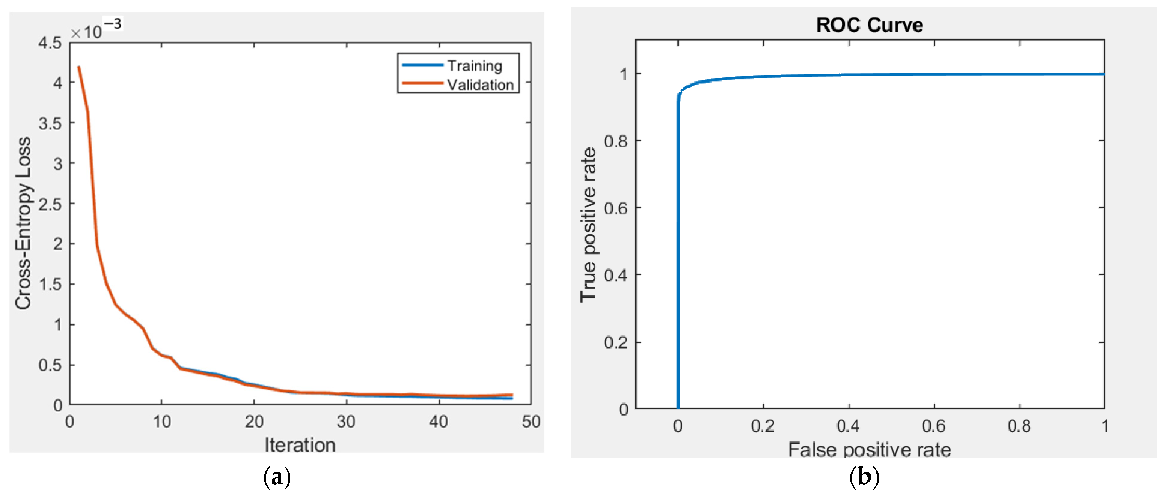
The results of the random sample calculation are shown in
Figure 10.
The collision detection accuracy obtained from the training results of Network 3 is summarized in
Table 9.
When trained on a larger dataset, the training results improved slightly, but still this network is not suitable for use. Since attempts to increase the complexity of the network itself and the size of the dataset do not yield a noticeable increase in training accuracy, further increases in the size of the dataset and the number of neurons will not yield the desired results. The network will constantly undertrain.
4.2. The ANN with Multi-Class (Three-Class) Classification
We will conduct research when adding the third class—Warning, which will allow us to take into account the situation in which, as noted above, the collision state (significant events) is less than 0.01% of the total number of states, since most of the manipulator positions are not in a self-collision state. The small number of significant events prevents the ANN algorithms from correctly predicting the collision state at other random values. To eliminate this problem, we discard some of the states that do not affect learning, which will increase the percentage of significant events in the sample.
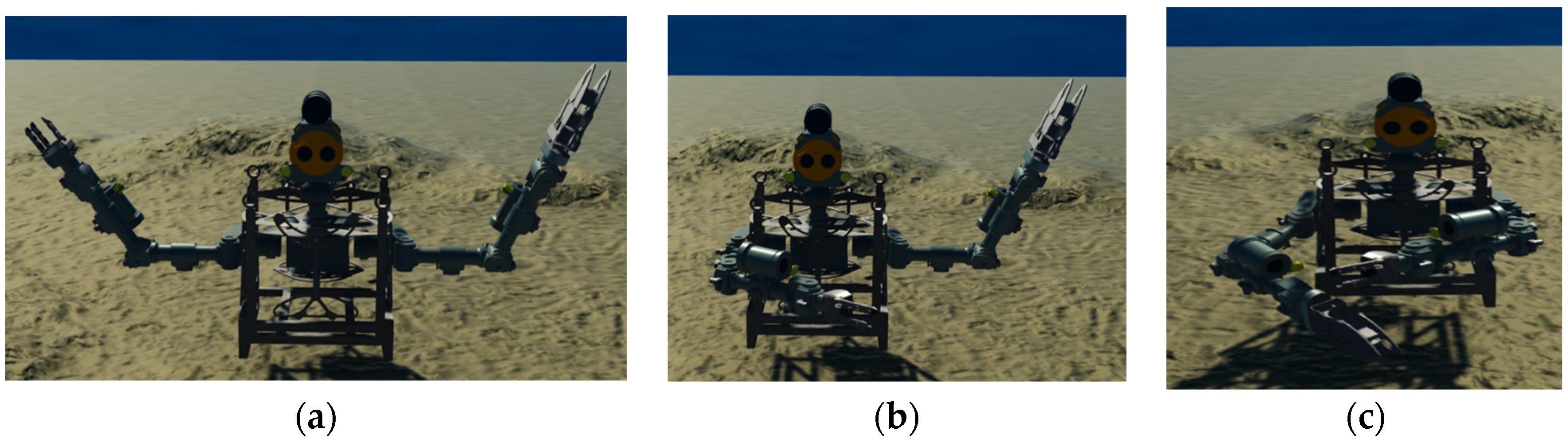
To determine the training dataset, we will compile 2000 random positions for each manipulator. For the combination “each manipulator with each”, we obtain 4,000,000 random positions. In the sample, we leave those cases when one or both manipulators fall along the X axis into a previously agreed corridor located in the center of the robot, or pass through it (
Figure 5b,c and
Figure 6b,c).
Figure 5a and
Figure 6a show the situation when data are excluded.
Based on these rules, let us compose Dataset 3 for training. For this purpose, we will select 73,984 values from 4,000,000 data according to our rules, 9062 of which will be collisions. The percentage of significant events to the rest of the values in the new samples was approximately 12%.
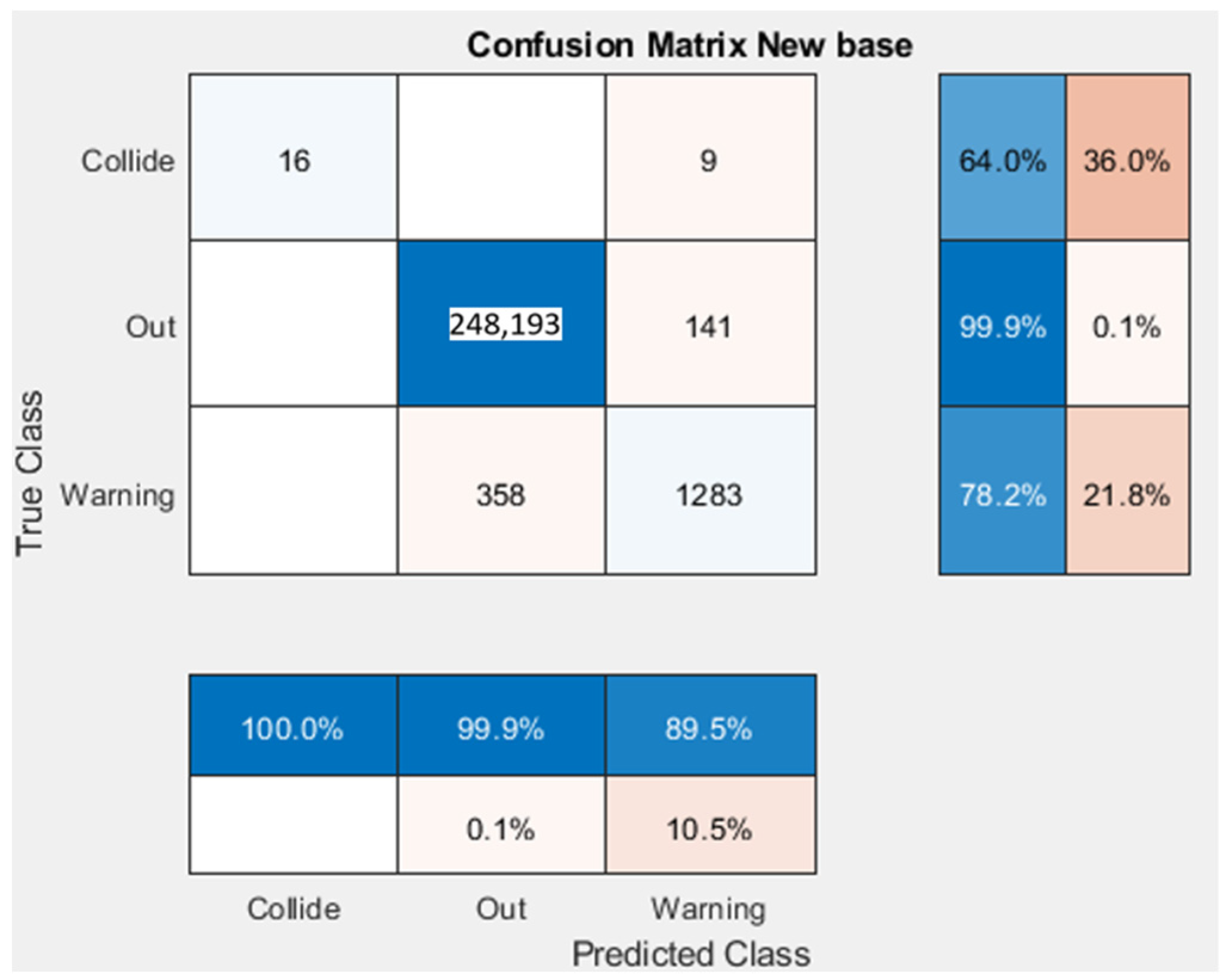
Let us consider Network 2 and use Dataset 3 to train it. Let us denote this network as Network 4.
The results of calculation on a random sample are shown in
Figure 11. The confusion matrix is shown in
Figure 12.
The results of the training are summarized in
Table 10.
The obtained result is much higher than the previous solutions. However, the obtained result is not satisfactory and, therefore, we will return to the consideration of the binary classification problem and tuning of the network parameters.
4.3. Changing the Training Method
In previous studies, the holdout validation method, which is recommended for use in large datasets [
28,
29,
30], was used to train Networks 1–4. The method consists of dividing the training data into two unequal parts. One part will be used to train the model and the second part will be used to validate the training. The advantage of the method is that there is no additional training cost and higher training speed compared to cross validation due to only one training. However, it is unknown which data from the total set will fall into the validation set, so the training result may be different for each random sample. This is partially compensated for by using a large sample of data. This reduces the probability that significant events are not evenly spaced, distorting the training sample, and, as a consequence, prevents a decrease in the quality of model training.
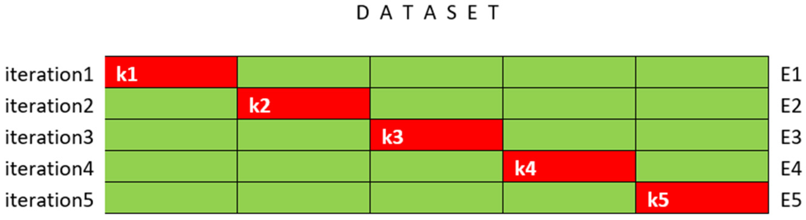
When separating the training data into training and testing areas, there is a risk of losing significant events in the training dataset and, as a result, obtaining a poorer model. Therefore, consider using the cross-validation method, which uses the same data points for training and testing. In the cross-validation method, the data are divided into k equal subsets. Training takes place k times such that each of the k subsets is used as a validation set, and the other subsets are combined to form the training set. The results of each training iteration are then added up and the average is found to obtain the generalized performance of the model.
Figure 13 shows an example of training data generation using cross-validation method divided into 5 subsets.
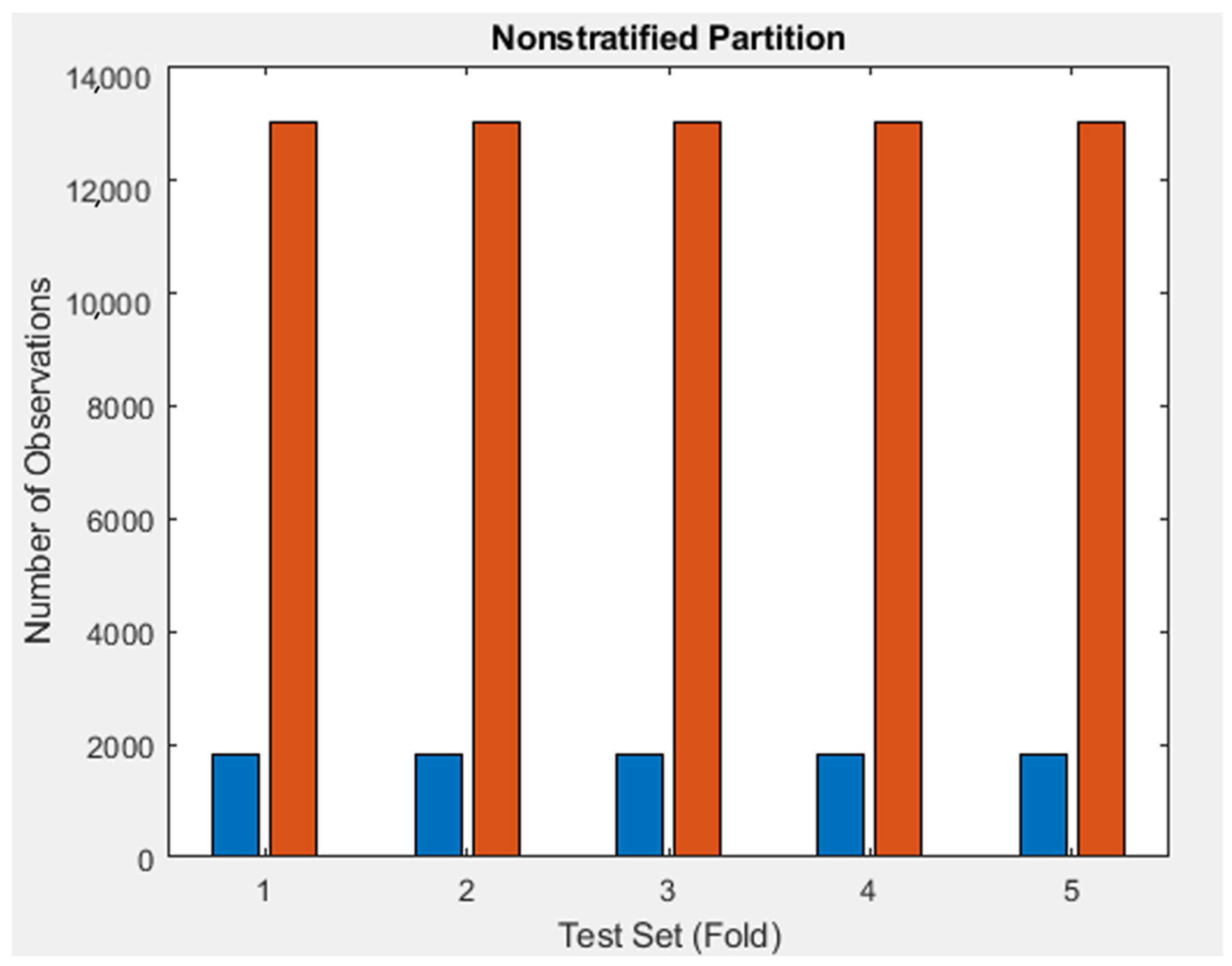
To determine the effectiveness of training the model using cross-validation method, train the model at k = 5. Create a model where 80% of the data are used for training and 20% for testing.
As a training sample, we use Dataset 3, which was divided into five parts and trained five times. Each time the test part was changed in such a way that all the data from Dataset3 participated in the training (
Figure 14 and
Figure 15). The parameters of the ANN (Network 5) are summarized in
Table 11.
Based on the obtained data, we can conclude that the network was trained with overfitting. According to the results of training, we obtained 100% accuracy on the training sample; however, when testing the network on another random sample, the collision prediction error increased to 5%. This variation indicates that the network is overfitting. The cross-validation method did not improve the learning situation, but rather led the system to overfitting. Moreover, the training time by this method increases directly proportional to the number of k values. The training time increased 5 times compared to the holdout validation method. Since no obvious improvement in learning was obtained using the cross-validation method, and based on the fact that the input data can be increased without limitation, without fear that some important part of the data will not be included in the training sample, we return to the holdout validation method for further research.
4.4. Regularization
To avoid the problem of overfitting, we add regularization to the ANN construction. Selecting the optimal value of the regularization parameter λ will allow us to achieve a balance between the simplicity of the model and the risk of overfitting. The larger λ is, the simpler the model is, but the predictions are worse. There will be a risk of underfitting. If λ is very small, the model will be highly complex and the risk of overfitting will increase. If λ is equal to zero, regularization is canceled and learning occurs only by minimizing the loss, this may lead to overfitting.
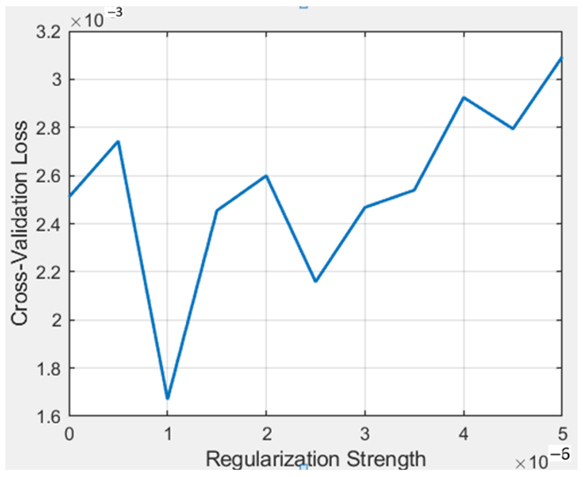
We test the performance of the model with different values of λ in the validation set, and choose the value of λ that gives the best result.
Appendix A contains a Matlab script that implements the algorithm that checks if the value of λ is found in the range of
.
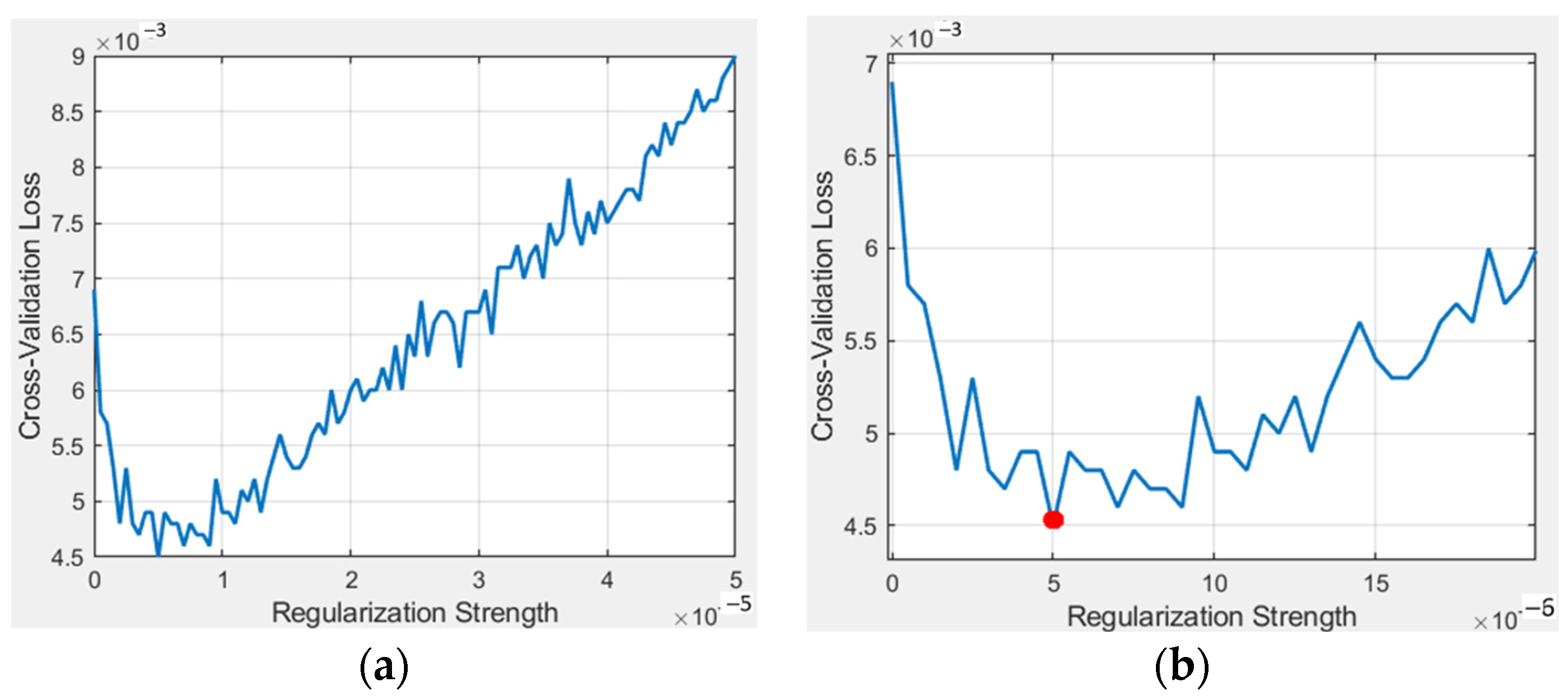
As a result, the regularization parameter corresponding to the lowest classification error equal to
(Illustrated with a red circle in
Figure 18).
Let us train the network (Network 6) using the obtained value of λ on Dataset 3. Network parameters are given in
Table 13.
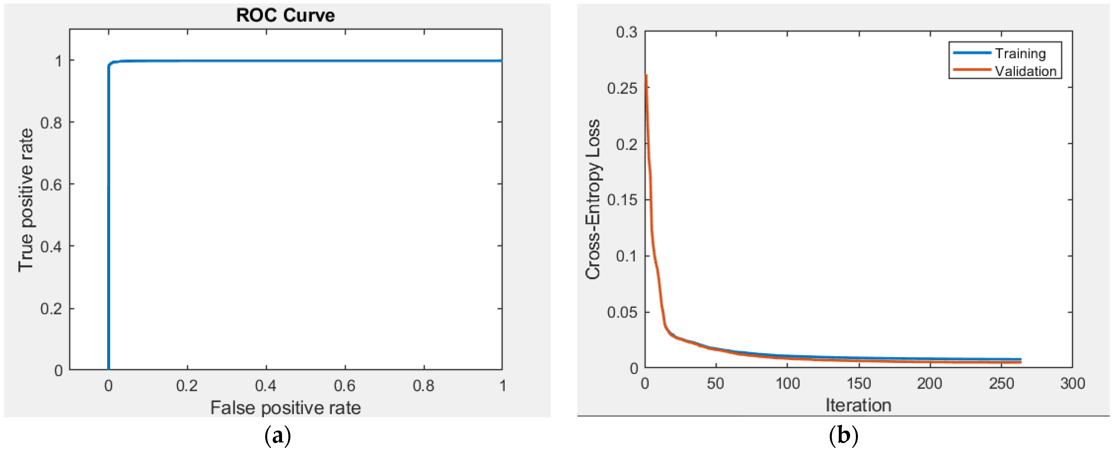
The result of the training is shown in
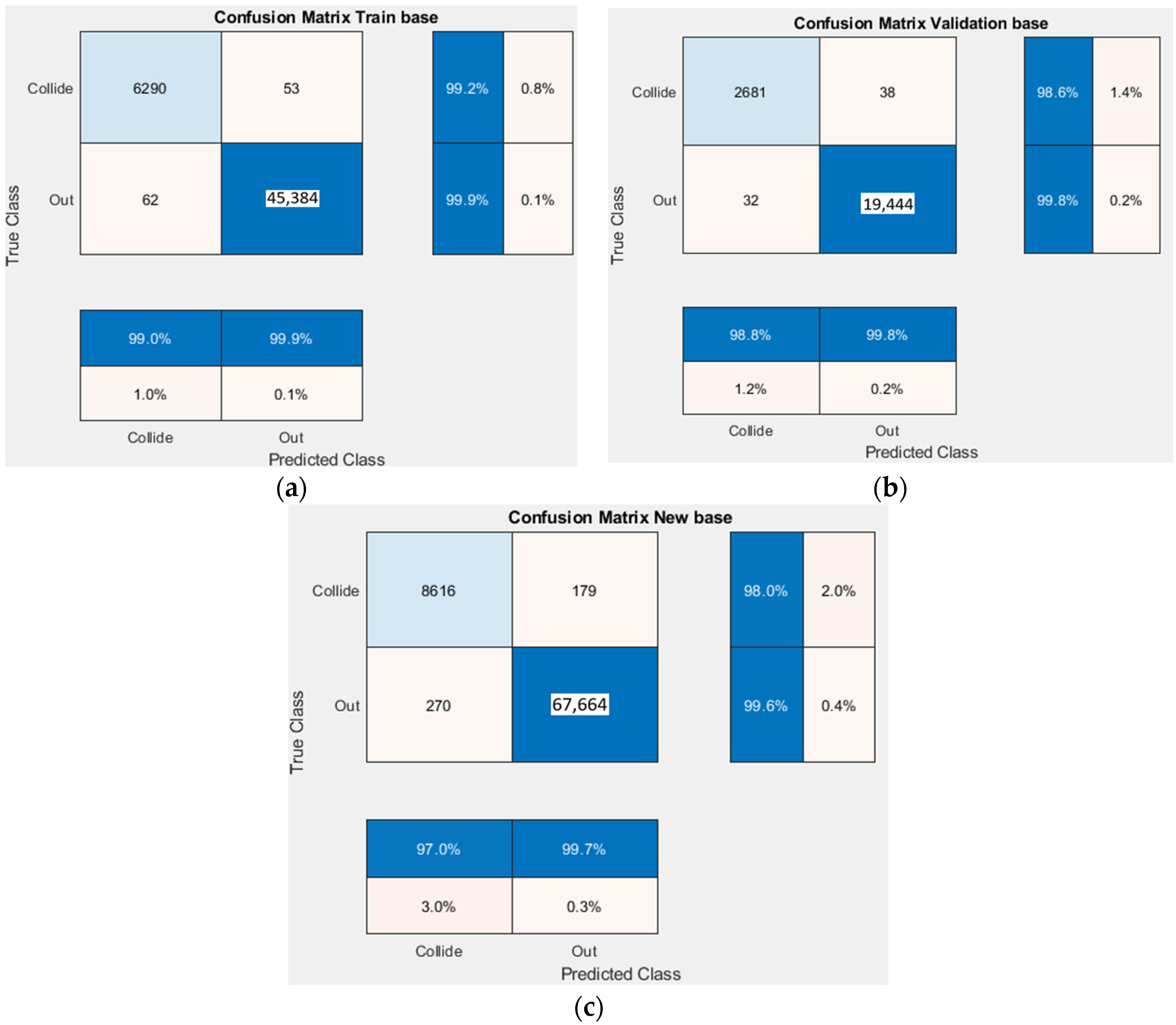
Figure 19. The confusion matrices are shown in
Figure 20. The results are summarized in
Table 14.
The result obtained by applying regularization is far superior to previous solutions.
We can improve the result by increasing dataset, i.e., adding more data to the training sample. This is the easiest and most feasible way to reduce the scatter. Let us prepare new data (Dataset 4) with 1,172,889 total values and 133,068 significant values that are collisions.
Since the input data have been changed, it is necessary to recalculate the regularization, since it depends on the input data. As before, we train the network with different values of λ (
Figure 21). As a result, we found the regularization parameter corresponding to the lowest classification error
.
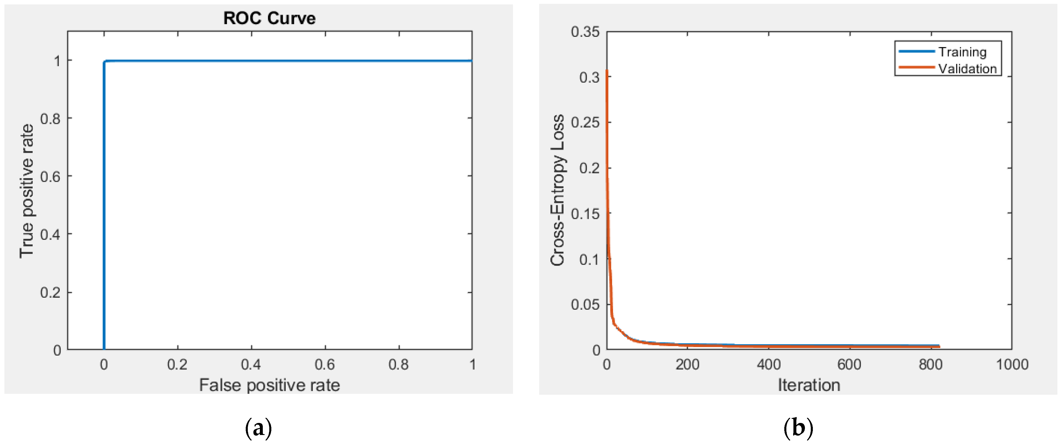
We derive the networks at the best value (Network 7) using the obtained value of λ on dataset with 1172889 total values and 133068 collisions being significant values.
The result obtained by applying regularization and augmented dataset shows a high result, in terms of prediction accuracy.
5. The Experimental Results
Let us apply the developed approaches to the analysis of self-collisions of robots with two multilink manipulators SAR-401 and “Ichtiandr”. Video of the experiments can be viewed at the link
https://youtu.be/Qw7ksK1NlHw accessed on 10 December 2023,
https://youtu.be/6v5OiB0T4B8 accessed on 10 December 2023.
We will conduct the experiment in three stages. Stage 1—testing the methods using a kinematic model built in Matlab. Stage 2—testing methods using simulators. Stage 3—testing the methods on real robots. Simulation of a self-collision at stage 3 was carried out using the actions of an operator in a copying suit to prevent the situation of the algorithm not working and the occurrence of a self-collision and damage to the robot.
The main problem of the experiment on a real robot is the risk of damage to the robot when the manipulators collide. Therefore, the main tests were carried out on a simulator and only when the ANN was developed was an experiment carried out on a real robot.
The appearance of the copying suits is shown in
Figure 1. A view of the operator in a suit is shown in
Figure 3.
The underwater robot was tested in a pool at a depth of 4 m. The control algorithm when working with real robots includes a self-collision control algorithm and a duplicate, previously developed algorithm based on solving the regression problem. This is due to the fact that the probability of detecting a self-collision using the developed algorithm is 2% and an unauthorized self-collision is possible, due to which they may break.
Having trained Network 7, we will perform all three stages of testing for each of the robots. In
Figure 24 and
Figure 25, the examples of experimental results are given. In
Figure 24 and
Figure 25, the right and left robot manipulators are indicated in red and blue, respectively.
Based on the results of a quantitative analysis of 2000 positions leading to self-collisions for the “Ichtiandr” robot, 1963 identified self-collisions were obtained, which gives 1.85% of unpredicted collisions, which is consistent with the results obtained.
Based on the results of a quantitative analysis of 2000 positions leading to self-collisions for the SAR-401 robot, 1968 identified self-collisions were obtained, which gives 1.6% of unpredicted collisions, which is consistent with the results obtained.
6. Discussion
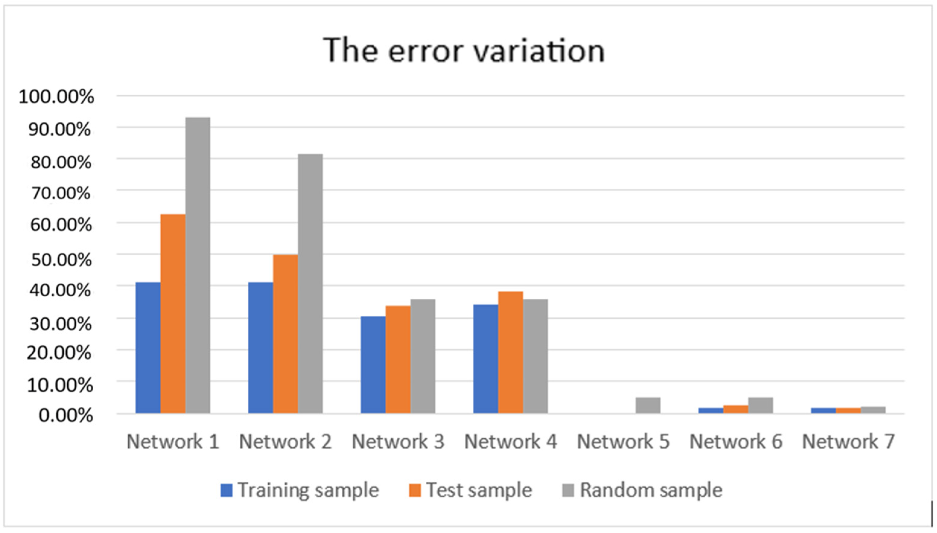
The generalized results of self-collision detection of two manipulators based on the classification ANN are summarized in
Table 16. The graph of the error variation is shown in
Figure 26. It should be noted once again that the characteristics of the most significant networks obtained during the design process are given in this paper.
Analyzing the obtained results, we can conclude that for correct operation and real application of the ANN, it is necessary to train them on a sufficiently large sample of input data, and the more input analyzed features, the higher the complexity of the network, the larger the sample should be.
A comparative analysis between the cross-validation method and the holdout method was performed. In spite of all the advantages of the cross-validation method for the considered problem of controlling the self-collision of multilink manipulators, the holdout method showed the best results.
The classification ANN can be applied to the collision detection solution, but even though the error is small, we still cannot neglect it because sooner or later it will lead to collision and damage the mechanism.
As mentioned above and in [
7], experimental approaches are often used when designing the ANN because of the difficulty in finding the global extremum. In [
14], it is shown that by constructing an efficient ANN configuration, a complex solution can be obtained that allows us to solve IKP and the self-collision control problem simultaneously with a high degree of speed and accuracy, either based on the solution of a regression problem or a classification problem.
Let us also evaluate the time characteristics. In [
7], it is stated that the time for calculating the classical solution of the IKP when calculating 400 points for a complex trajectory was from 33 to 42 s. The analytical solution of the self-collision analysis problem under the condition that 400 points for a complex trajectory are selected is approximately the same time—40–45 s.
The solution to the manipulator self-collision analysis problem for the proposed ANN was as follows: Network 1 time is 0.005601 s, Network 2 time is 0.005074 s, Network 3 time is 0.015788 s, Network 4 time is 0.067734 s, Network 5 time is 0.160974 s, Network 6 time is 0.005566 s, Network 7 time is 0.005766 s. This is much faster than using the classical approach. Calculations were carried out on a PC Intel CORE-i9@2.9GHz/64 G/NVIDIA Quadro P5000, DS-Systems, Beijing, China.
As a result of our research, we were able to develop the ANN based on a classification approach that was able to predict manipulator collisions with 98% accuracy.
The proposed approach can be scaled to any type of multilink manipulators, as well as to robots with more than two manipulators. And, as noted above, it will prevent damage to robots with multilink manipulators when they perform complex technological operations. As for the scalability of the results, we assume that for multilink manipulators with a kinematic scheme similar to the “Ichtiandr” and SAR-401 robots, the proposed approach will show its effectiveness. In this case, it is necessary to build your own dataset and adjust the network parameters. As for the operating environment of the manipulators, the approach proposed in this article provides almost identical results for the “Ichtiandr” robots (works underwater) and SAR-401 (works in a normal environment).
At the same time, it should be noted that the limitation of the method is not 100% accurate in predicting the possibility of a self-collision. Despite the high accuracy of the prediction method, there is a small percentage (no more than 2%) that the algorithm gives an erroneous prediction. Therefore, when implementing a self-collision control algorithm using the ANN approach to prevent damage to manipulators, taking into account the high speed of the algorithms, it is necessary to simultaneously use an approach based on a regression task and based on a classification task. The simultaneous operation of the algorithms will determine the outcome of the forecast.
To implement the developed method, a C# program was developed that uses a developed ANN based on classification approaches for collision avoidance.
In the control system, commands from the control program are transmitted to the collision testing program, where collisions are analyzed and predicted not only in the final position of the manipulators, but also along the entire movement path. If a collision is not predicted, the command is passed on to the robot. If a collision has been predicted, the command to move the manipulator is not transmitted to the robot and thus the collision is prevented.
Author Contributions
Conceptualization V.K., O.K. and A.K.; methodology, V.K. and O.K.; software, O.K.; validation, V.K. and V.A.; formal analysis, A.K.; investigation, V.K. and O.K.; resources, A.K.; data curation, O.K.; writing—original draft preparation, V.K. and O.K.; writing—review and editing, V.K.; visualization, V.K.; supervision, A.K. and V.A.; project administration, A.K.; funding acquisition, A.K. All authors have read and agreed to the published version of the manuscript.
Funding
This research received no external funding.
Institutional Review Board Statement
Ethical review and approval were waived through the Ethical Committee of Sevastopol State University for this study, due to animals or people as an object study not recorded.
Informed Consent Statement
Informed consent was obtained from all subjects involved in the study.
Data Availability Statement
The data presented in this study are available upon request from the corresponding author. The data are not publicly available due to privacy.
Conflicts of Interest
The authors declare no conflict of interest.
Appendix A
| Algorithm A1 for finding λ in the range |
lambda = (0:0.5:50)*1 × 10−6;
cvloss = zeros(length(lambda),1);
for i = 1:length(lambda)
Mdl = fitcnet(tblTrain,”Y”, …
“ValidationData”,tblValidation, …
“Verbose”,1, …
“Activations”, ‘sigmoid’, …
“LayerSizes”,47,…
“Standardize”, true, …
“ClassNames”, categorical({‘Collide’; ‘Out’}),…
“Lambda”, lambda(i) …
);
cvloss(i) = loss(Mdl,tblTrain(:,1:24),tblTrain.Y, …
“LossFun”,”classiferror”)
end
[~,idx] = min(cvloss);
bestLambda = lambda(idx) |
References
- Robla-Gomez, S.; Becerra, V.M.; Llata, J.R.; Gonzalez-Sarabia, E.; Torre-Ferrero, C.; Perez-Oria, J. Working Together: A review on safe human-robot collaboration in industrial environments. IEEE Access 2017, 5, 26754–26773. [Google Scholar] [CrossRef]
- Siciliano, B.; Khatib, O. Springer Handbook of Robotics; Springer: Berlin/Heidelberg, Germany, 2008. [Google Scholar]
- Liao, Z.; Jiang, G.; Zhao, F.; Mei, X.; Yue, Y. A novel solution of inverse kinematic for 6R robot manipulator with offset joint based on screw theory. Int. J. Adv. Robot. Syst. 2020, 17, 1729881420925645. [Google Scholar] [CrossRef]
- Yuh, J.; Marani, G.; Blidberg, R. Applications of marine robotic vehicles. Intell. Serv. Robot. 2011, 4, 221–231. [Google Scholar] [CrossRef]
- Corke, P.I. Robotics, Vision and Control Fundamental Algorithms in Matlab; Springer: Cham, Switzerland, 2017; p. 693. [Google Scholar] [CrossRef]
- Bogdanov, A.; Dudorov, E.; Permyakov, A.; Pronin, A.; Kutlubaev, I. Control system of a manipulator of the anthropomorphic robot Fedor. In Proceedings of the International Conference on Developments in eSystems Engineering, DeSE, Kazan, Russia, 7–10 October 2019; pp. 449–453. [Google Scholar] [CrossRef]
- Kramar, V.; Kramar, O.; Kabanov, A. An Artificial Neural Network Approach for Solving Inverse Kinematics Problem for an Anthropomorphic Manipulator of Robot SAR-401. Machines 2022, 10, 241. [Google Scholar] [CrossRef]
- Bogdanov, A.; Kutlubaev, I.; Permyakov, A.; Sychkov, V. Development of an anthropomorphic robot with an interactive control. In Proceedings of the VIII All-Russian Conference, Moscow, Russia, 27–29 January 2015; pp. 228–230. [Google Scholar]
- Li, S.; Zhang, Y.; Jin, L. Kinematic Control of Redundant Manipulators Using Neural Networks. IEEE Trans. Neural Netw. Learn. Syst. 2017, 28, 2243–2254. [Google Scholar] [CrossRef] [PubMed]
- Ahmed, R.J.; Almusawi, L.; Dülger, C.; Kapucu, S. A New Artificial Neural Network Approach in Solving Inverse Kinematics of Robotic Arm. Comput. Intell. Neurosci. 2016, 2016, 5720163. [Google Scholar] [CrossRef]
- Crenganiş, M.; Breaz, R.; Racz, G.; Bologa, O. The inverse kinematics solutions of a 7 DOF robotic arm using fuzzy logic. In Proceedings of the 7th IEEE Conference on Industrial Electronics and Applications, Singapore, 18–20 July 2012; pp. 518–523. [Google Scholar] [CrossRef]
- Liu, J.; Wang, Y.; Li, B.; Ma, S. Neural Network Based Kinematic Control of the Hyper-Redundant Snake-Like Manipulator. In Proceedings of the 4th International Symposium on Neural Networks, Nanjing, China, 3–7 June 2007. [Google Scholar] [CrossRef]
- Daya, B.; Khawandi, S.; Akoum, M. Applying neural network architecture for inverse kinematics problem in robotics. J. Softw. Eng. Appl. 2010, 3, 230–239. [Google Scholar] [CrossRef]
- Kramar, V.; Kramar, O.; Kabanov, A. Self-Collision Avoidance Control of Dual-Arm Multi-Link Robot Using Neural Network Approach. J. Robot. Control 2022, 3, 309–3191. [Google Scholar] [CrossRef]
- Mendili, M.; Bouani, F. Predictive Control of Mobile Robot Using Kinematic and Dynamic Models. J. Control. Sci. Eng. 2017, 2017, 5341381. [Google Scholar] [CrossRef]
- Sivcev, S.; Rossi, M.; Coleman, J.; Omerdic, E.; Dooly, G.; Toal, D. Collision detection for underwater ROV manipulator systems. Sensors 2018, 18, 1117. [Google Scholar] [CrossRef] [PubMed]
- Santis, A.; Albu-Schäffer, A.; Ott, C.; Siciliano, B.; Hirzinger, G. The skeleton algorithm for real-time collision avoidance of a humanoid manipulator inter-acting with humans. In Proceedings of the 2007 IEEE/ASME International Conference on Advanced Intelligent Mechatronics, Zurich, Switzerland, 4–7 September 2007; p. 9871732. [Google Scholar]
- Wu, D.; Yu, Z.; Adili, A.; Zhao, F. A Self-Collision Detection Algorithm of a Dual-Manipulator System Based on GJK and Deep Learning. Sensors 2023, 23, 523. [Google Scholar] [CrossRef] [PubMed]
- Liu, Z.; Zhang, L.; Qin, X.; Li, G. An effective self-collision detection algorithm for multi-degree-of-freedom manipulator. Meas. Sci. Technol. 2023, 34, 015901. [Google Scholar] [CrossRef]
- Arents, J.; Abolins, V.; Judvaitis, J.; Vismanis, O.; Oraby, A.; Ozols, K. Human–robot collaboration trends and safety aspects: A systematic review. J. Sens. Actuator Netw. 2021, 10, 48. [Google Scholar] [CrossRef]
- Park, K.W.; Kim, M.; Kim, J.S.; Park, J.H. Path planning for multi-Arm Manipulators using Soft Actor-Critic algorithm with position prediction of moving obstacles via LSTM. Appl. Sci. 2022, 12, 9837. [Google Scholar] [CrossRef]
- Kramar, V.; Kabanov, A.; Alchakov, V. Application of Linear Algebra Approaches for Predicting Self-Collisions of Dual-Arm Multi-Link Robot. Int. J. Mech. Eng. Robot. Res. 2020, 9, 1521–1525. [Google Scholar] [CrossRef]
- Pan, T.Y.; Wells, A.M.; Shome, R.; Kavraki, L.E. A general task and motion planning framework for multiple manipulators. In Proceedings of the International Conference on Intelligent Robots and Systems (IROS), Electronic Network, Prague, Czech Republic, 27 September–1 October 2021; pp. 3168–3174. [Google Scholar]
- Tian, X.; Xu, Q.; Zhan, Q. An analytical inverse kinematics solution with joint limits avoidance of 7-DOF anthropomorphic manipulators without offset. J. Frankl. Inst. 2021, 358, 1252–1272. [Google Scholar] [CrossRef]
- Lei, M.; Wang, T.; Yao, C.; Liu, H.; Wang, Z.; Deng, Y. Real-time kinematics-based self-collision avoidance algorithm for dual-arm robots. Appl. Sci. 2020, 10, 5893. [Google Scholar] [CrossRef]
- Jang, K.; Kim, S.; Park, J. Reactive self-collision avoidance for a differentially driven mobile manipulator. Sensors 2021, 21, 890. [Google Scholar] [CrossRef] [PubMed]
- Denavit, J.; Hartenberg, R.S. A Kinematic Notation for Lower-Pair Mechanisms Based on Matrices. J. Appl. Mech. Trans. ASME 1955, 22, 215–221. [Google Scholar] [CrossRef]
- Ng, A. Machine Learning Yearning; GitHub eBook (MIT Licensed): San Francisco, CA, USA, 2018; p. 118. [Google Scholar]
- Mueller, A.C.; Guido, S. An Introduction to Machine Learning with Python; O’Reilly Australia & New Zealand: Sebastopol, CA, USA, 2017. [Google Scholar]
- Witten Ian, H.; Eibe, F.; Hall Mark, A.; Pal Christopher, J. Data Mining: Practical Machine Learning Tools and Techniques; Elsevier: Amsterdam, The Netherlands, 2017. [Google Scholar] [CrossRef]
Figure 1.
Robot “Ichtiandr”: (a) the general view of the robot; (b) copy suit.
Figure 1.
Robot “Ichtiandr”: (a) the general view of the robot; (b) copy suit.
Figure 2.
The torso anthropomorphic robot SAR-401: (a) the general view of the robot; (b) copy suit.
Figure 2.
The torso anthropomorphic robot SAR-401: (a) the general view of the robot; (b) copy suit.
Figure 3.
The control scheme with the copying suit.
Figure 3.
The control scheme with the copying suit.
Figure 4.
The kinematic scheme of the left manipulator.
Figure 4.
The kinematic scheme of the left manipulator.
Figure 5.
State of classes for the SAR-401 robot: (a) Out class; (b) Warning class; (c) Collide class.
Figure 5.
State of classes for the SAR-401 robot: (a) Out class; (b) Warning class; (c) Collide class.
Figure 6.
State of classes for the “Ichtiandr” robot: (a) Out class; (b) Warning class; (c) Collide class.
Figure 6.
State of classes for the “Ichtiandr” robot: (a) Out class; (b) Warning class; (c) Collide class.
Figure 7.
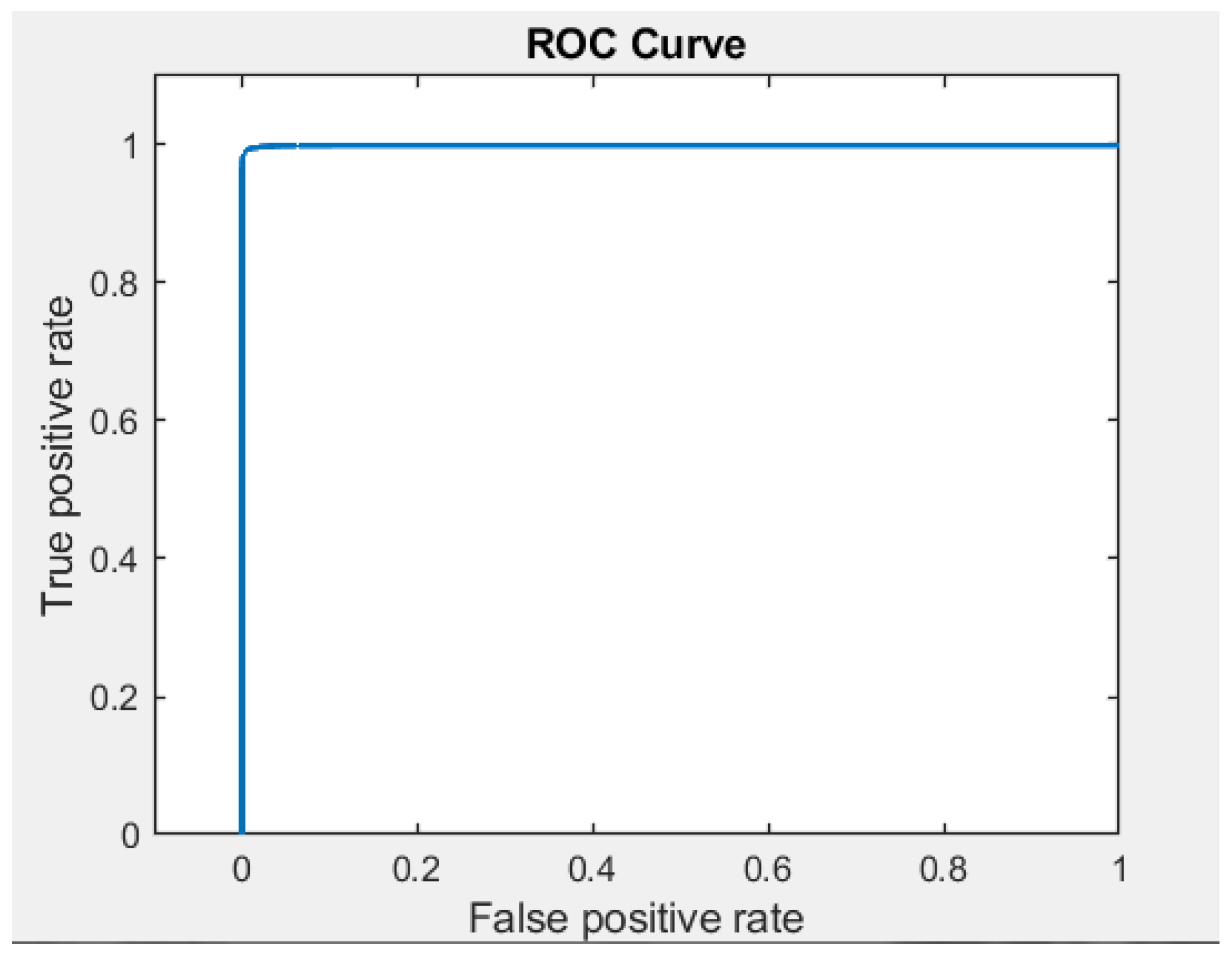
The results of training Dataset 1 on the raw sample (a) cross-entropy loss; (b) true positive rate.
Figure 7.
The results of training Dataset 1 on the raw sample (a) cross-entropy loss; (b) true positive rate.
Figure 8.
The confusion matrix (a) for the training sample; (b) for the test sample; (c) for the random sample.
Figure 8.
The confusion matrix (a) for the training sample; (b) for the test sample; (c) for the random sample.
Figure 9.
Results of Network 2 training on a random sample (a) cross-entropy loss; (b) true positive rate.
Figure 9.
Results of Network 2 training on a random sample (a) cross-entropy loss; (b) true positive rate.
Figure 10.
Results of Network 3 training on a random sample (a) cross-entropy loss; (b) true positive rate.
Figure 10.
Results of Network 3 training on a random sample (a) cross-entropy loss; (b) true positive rate.
Figure 11.
Results of Network 4 training on a random sample (a) cross-entropy loss; (b) true positive rate.
Figure 11.
Results of Network 4 training on a random sample (a) cross-entropy loss; (b) true positive rate.
Figure 12.
The confusion matrix.
Figure 12.
The confusion matrix.
Figure 13.
Example of training data generation using cross-validation method divided into 5 subsets.
Figure 13.
Example of training data generation using cross-validation method divided into 5 subsets.
Figure 14.
Five-fold cross-validation partition (blue indicates TestSize, red indicates TrainSize).
Figure 14.
Five-fold cross-validation partition (blue indicates TestSize, red indicates TrainSize).
Figure 15.
A fragment of the creation of training sets.
Figure 15.
A fragment of the creation of training sets.
Figure 16.
Result of training of Network 5.
Figure 16.
Result of training of Network 5.
Figure 17.
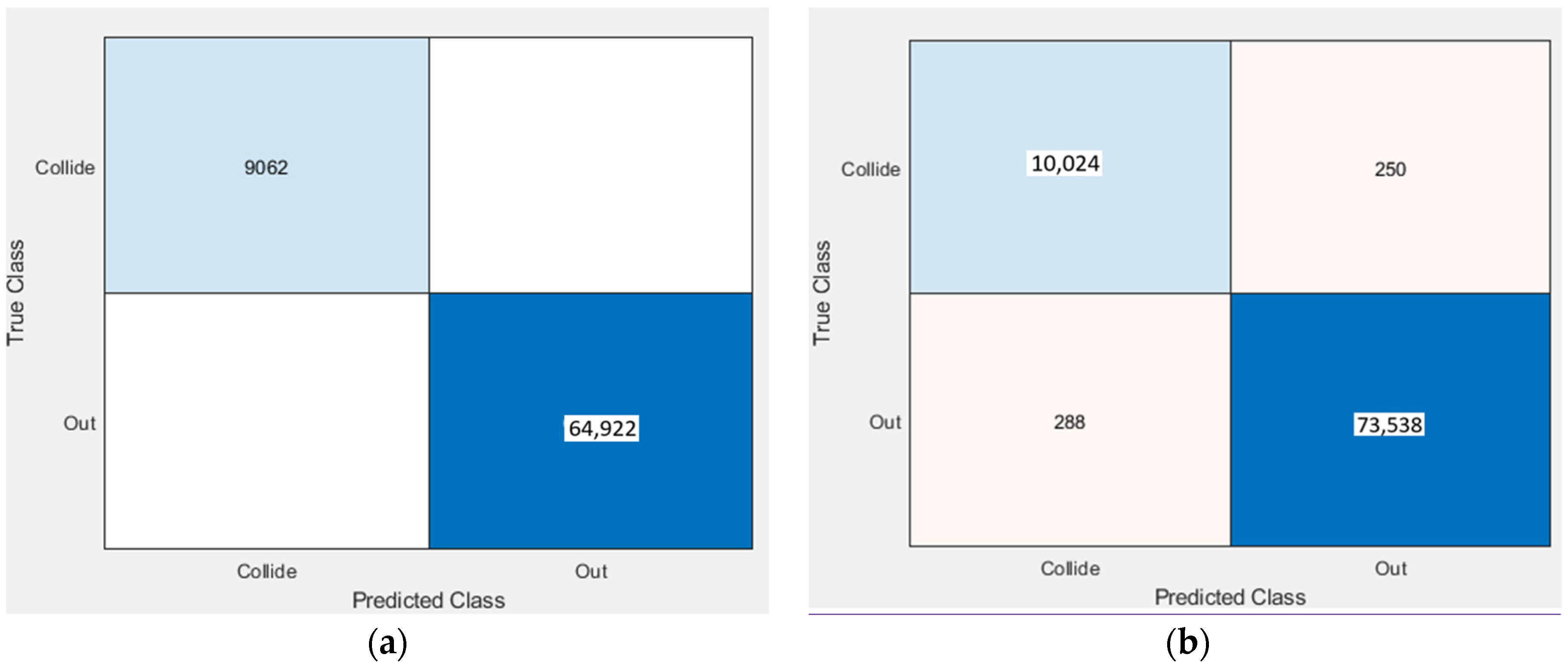
The confusion matrices (a) for the training sample; (b) for the random sample.
Figure 17.
The confusion matrices (a) for the training sample; (b) for the random sample.
Figure 18.
Changing the regularization parameter (a) general view; (b) enlarged fragment.
Figure 18.
Changing the regularization parameter (a) general view; (b) enlarged fragment.
Figure 19.
The result of the training Network 6 (a) model accuracy; (b) model loss.
Figure 19.
The result of the training Network 6 (a) model accuracy; (b) model loss.
Figure 20.
The confusion matrices (a) for the training sample; (b) for the test sample; (c) for the random sample.
Figure 20.
The confusion matrices (a) for the training sample; (b) for the test sample; (c) for the random sample.
Figure 21.
Changing the regularization parameter.
Figure 21.
Changing the regularization parameter.
Figure 22.
The result of the training Network 7 (a) model accuracy; (b) model loss.
Figure 22.
The result of the training Network 7 (a) model accuracy; (b) model loss.
Figure 23.
The confusion matrix.
Figure 23.
The confusion matrix.
Figure 24.
The experimental results “Ichtiandr”: (a) Matlab model; (b) simulator; (c) real robot.
Figure 24.
The experimental results “Ichtiandr”: (a) Matlab model; (b) simulator; (c) real robot.
Figure 25.
The experimental results SAR-401: (a) Matlab model; (b) simulator; (c) real robot.
Figure 25.
The experimental results SAR-401: (a) Matlab model; (b) simulator; (c) real robot.
Figure 26.
The graph of the error variation.
Figure 26.
The graph of the error variation.
Table 1.
The DH parameters for the left manipulator.
Table 1.
The DH parameters for the left manipulator.
| Link, i | | | | |
|---|
| 1 | 0 | π/2 | 0 | |
| 2 | 0 | π/2 | 0 | |
| 3 | 0 | π/2 | −0.3 | |
| 4 | 0 | π/2 | 0 | |
| 5 | 0 | π/2 | −0.3 | |
| 6 | −0.24 | 0 | 0 | |
Table 2.
Servo limits.
| № | Min Left | Max Left | Min Right | Max Right |
|---|
| 0 | −90° | 0° | −90° | 0° |
| 1 | 0° | 105° | −105° | 0° |
| 2 | −40° | 40° | −40° | 40° |
| 3 | −110° | 5° | −110° | 5° |
| 4 | −40° | 40° | −40° | 40° |
| 5 | −10° | 10° | −10° | 10° |
Table 3.
The input parameters characterizing the position in space of each manipulator.
Table 3.
The input parameters characterizing the position in space of each manipulator.
| Left manipulator | Lnx | 0.51 | 0.51 | 0.51 | 0.51 | 0.51 | 0.51 | 0.51 | 0.51 | 0.51 | 0.51 | 0.51 | 0.51 | 0.51 |
| Lox | 0.56 | 0.56 | 0.56 | 0.56 | 0.56 | 0.56 | 0.56 | 0.56 | 0.56 | 0.56 | 0.56 | 0.56 | 0.56 |
| Lax | −0.65 | −0.65 | −0.65 | −0.65 | −0.65 | −0.65 | −0.65 | −0.65 | −0.65 | −0.65 | −0.65 | −0.65 | −0.65 |
| Lx | −0.36 | −0.36 | −0.36 | −0.36 | −0.36 | −0.36 | −0.36 | −0.36 | −0.36 | −0.36 | −0.36 | −0.36 | −0.36 |
| Lny | 0.83 | 0.83 | 0.83 | 0.83 | 0.83 | 0.83 | 0.83 | 0.83 | 0.83 | 0.83 | 0.83 | 0.83 | 0.83 |
| Lox | 0.43 | 0.43 | 0.43 | 0.43 | 0.43 | 0.43 | 0.43 | 0.43 | 0.43 | 0.43 | 0.43 | 0.43 | 0.43 |
| Lax | 0.78 | 0.78 | 0.78 | 0.78 | 0.78 | 0.78 | 0.78 | 0.78 | 0.78 | 0.78 | 0.78 | 0.78 | 0.78 |
| Ly | 0.02 | 0.02 | 0.02 | 0.02 | 0.02 | 0.02 | 0.02 | 0.02 | 0.02 | 0.02 | 0.02 | 0.02 | 0.02 |
| Lnz | 0.63 | 0.63 | 0.63 | 0.63 | 0.63 | 0.63 | 0.63 | 0.63 | 0.63 | 0.63 | 0.63 | 0.63 | 0.63 |
| Lox | −0.02 | −0.02 | −0.02 | −0.02 | −0.02 | −0.02 | −0.02 | −0.02 | −0.02 | −0.02 | −0.02 | −0.02 | −0.02 |
| Lax | −0.51 | −0.51 | −0.51 | −0.51 | −0.51 | −0.51 | −0.51 | −0.51 | −0.51 | −0.51 | −0.51 | −0.51 | −0.51 |
| Lz | 0.08 | 0.08 | 0.08 | 0.08 | 0.08 | 0.08 | 0.08 | 0.08 | 0.08 | 0.08 | 0.08 | 0.08 | 0.08 |
| Right manipulator | Rnx | 0.45 | 0.70 | −0.62 | −0.65 | −0.57 | 0.99 | 0.71 | −0.52 | 0.36 | 0.10 | 0.34 | −0.48 | 0.16 |
| Rox | 0.21 | 0.66 | 0.70 | 0.05 | 0.11 | 0.15 | 0.59 | 0.07 | 0.46 | 0.98 | 0.86 | 0.74 | 0.33 |
| Rax | −0.87 | −0.27 | −0.34 | −0.76 | −0.81 | −0.04 | −0.39 | −0.85 | −0.81 | 0.17 | 0.37 | −0.47 | −0.93 |
| Rx | 0.01 | 0.21 | −0.15 | −0.10 | 0.26 | 0.05 | 0.69 | 0.09 | −0.06 | 0.80 | 0.11 | −0.38 | 0.99 |
| Rny | 0.97 | 0.17 | 0.32 | 0.98 | 0.97 | −0.12 | −0.47 | 1.00 | 0.88 | −0.18 | −0.43 | 0.30 | −0.10 |
| Rox | 0.24 | 0.96 | 0.94 | 0.15 | −0.04 | 0.99 | 0.55 | 0.02 | 0.48 | 0.57 | 0.90 | 0.87 | 0.14 |
| Rax | 0.89 | 0.68 | 0.77 | 0.75 | 0.78 | 0.15 | 0.14 | 0.85 | 0.93 | 0.59 | 0.93 | 0.79 | −0.04 |
| Ry | −0.12 | −0.73 | 0.63 | 0.17 | −0.23 | −0.98 | −0.66 | −0.07 | −0.12 | 0.08 | −0.27 | 0.60 | −0.94 |
| Rnz | 0.43 | −0.02 | −0.10 | −0.64 | −0.58 | −0.13 | −0.74 | −0.52 | 0.34 | −0.80 | −0.24 | 0.14 | −0.34 |
| Rox | −0.50 | −0.85 | 0.06 | 0.05 | 0.07 | −1.06 | −0.93 | 0.03 | −0.53 | −0.40 | −0.59 | 0.02 | −0.62 |
| Rax | −0.37 | −0.51 | −0.39 | −0.31 | −0.34 | −0.13 | −0.30 | −0.36 | −0.48 | −0.55 | −0.60 | −0.62 | −0.13 |
| Rz | 0.36 | 0.04 | −0.14 | 0.40 | 0.43 | 0.01 | 0.18 | 0.46 | 0.37 | −0.33 | −0.39 | 0.06 | 0.56 |
| Class | Out | Out | Collide | Out | Out | Out | Out | Out | Out | Out | Out | Collide | Out |
Table 4.
The Network 1 parameters.
Table 4.
The Network 1 parameters.
| Parameter | Value |
|---|
| Layer activation function | sigmoid |
| Output layer activation function | softmax |
| Error search method | Cross-Entropy Loss |
| Hidden layers | 1 |
| The number of neurons | 10 |
| Training method | holdout validation |
| Learning function | LBFGS |
| Number of epochs | 1000 |
| Number of inputs | 24 |
| Number of output | 1 |
| GradientTolerance: | 1 × 10⁻⁶ |
| LossTolerance: | 1 × 10⁻⁶ |
| StepTolerance: | 1 × 10⁻⁶ |
| Classes | Out, Collide |
Table 5.
Input data.
| | Total Number of Values | Number of Collisions |
|---|
| Dataset1 | 250,000 | 25 |
| Dataset2 | 1,000,000 | 255 |
Table 6.
Absolute accuracy values (Accuracy).
Table 6.
Absolute accuracy values (Accuracy).
| Accuracy |
|---|
| on the training sample | on the test sample | on a random sample |
| 99.9% | 99.99% | 99.97% |
Table 7.
Accuracy of collision detection in Network 1.
Table 7.
Accuracy of collision detection in Network 1.
| | Training Sample | Test Sample | Random Sample |
|---|
| Precision | 81.25% | 100% | 53.78% |
| Recall | 76.47% | 37.5% | 50.19% |
| Error | 41.17% | 62.5% | 92.94% |
Table 8.
Accuracy of collision detection in Network 2.
Table 8.
Accuracy of collision detection in Network 2.
| | Training Sample | Test Sample | Random Sample |
|---|
| Precision | 81.25% | 100% | 61.03% |
| Recall | 76.47% | 50% | 50.98% |
| Error | 41.1% | 50% | 81.5% |
Table 9.
Accuracy of collision detection in Network 3.
Table 9.
Accuracy of collision detection in Network 3.
| | Training Sample | Test Sample | Random Sample |
|---|
| Precision | 86.90% | 84% | 94.44% |
| Recall | 82.02% | 81.81% | 68% |
| Error | 30.33% | 33.76% | 36% |
Table 10.
Accuracy of collision detection in Network 4.
Table 10.
Accuracy of collision detection in Network 4.
| | Training Sample | Test Sample | Random Sample |
|---|
| Precision | 98.59% | 98.23% | 95.95% |
| Recall | 98.78% | 98.08% | 97.55% |
| Error | 2.61% | 3.67% | 6.56% |
Table 11.
The Network 5 parameters.
Table 11.
The Network 5 parameters.
| Parameter | Value |
|---|
| Layer activation function | sigmoid |
| Hidden layers | 1 |
| The number of neurons | 47 |
| Training method | cross validation |
| Input dataset | Dataset3 |
Table 12.
Results of training of Network 5.
Table 12.
Results of training of Network 5.
| | Training Sample | Random Sample |
|---|
| Actual number of collisions | 9062 | 10,274 |
| Predicted collisions total | 9062 | 10,312 |
| Total errors | 0 | 538 |
| No collisions detected | 0 | 250 |
| Predicted false collisions | 0 | 288 |
Table 13.
The Network 6 parameters.
Table 13.
The Network 6 parameters.
| Parameter | Value |
|---|
| Layer activation function | sigmoid |
| Output layer activation function | softmax |
| Error search method | Cross-Entropy Loss |
| Hidden layers | 1 |
| The number of neurons | 47 |
| λ | 5 × 10⁻⁶ |
| Training method | holdout validation |
| Input dataset | Dataset3 |
| Learning function | LBFGS |
| Number of epochs | 1000 |
| Number of inputs | 24 |
| Number of output | 1 |
| GradientTolerance: | 1 × 10⁻⁶ |
| LossTolerance: | 1 × 10⁻⁶ |
| StepTolerance: | 1 × 10⁻⁶ |
Table 14.
Accuracy of collision detection in Network 6.
Table 14.
Accuracy of collision detection in Network 6.
| | Training Sample | Test Sample | Random Sample |
|---|
| Precision | 99.02% | 98.82% | 96.96% |
| Recall | 99.16% | 98.60% | 97.96% |
| Error | 1.8% | 2.57% | 5.10% |
Table 15.
Accuracy of collision detection in Network 7.
Table 15.
Accuracy of collision detection in Network 7.
| | Training Sample | Test Sample | Random Sample |
|---|
| Precision | 99.30% | 99.15% | 99.17% |
| Recall | 99.19% | 99.01% | 98.81% |
| Error | 1.50% | 1.84% | 2.00% |
Table 16.
The generalized results of self-collision detection.
Table 16.
The generalized results of self-collision detection.
| № Network | Prediction Error | Notes | Conclusion |
|---|
| Training Sample | Test Sample | Random Sample |
|---|
| Network 1 | 41.17% | 62.5% | 92.94% | A basic network with one layer and 10 neurons in it was used | Bad result, on a random dataset 92% incorrect results |
| Network 2 | 41.1% | 50% | 81.5% | Increased the number of neurons in the hidden layer to 47 | Bad result, on a random dataset 81.5% incorrect results |
| Network 3 | 30.33% | 33.76% | 36% | Increased dataset | 36% incorrect results, a change in the network is needed |
| Network 4 | 34.07% | 38.15% | 36% | Adding a third class | 36% incorrect results, a change in the network is needed |
| Network 5 | 0% | 0% | 5% | Changing the cross-validation training method | Received retraining |
| Network 6 | 1.8% | 2.57% | 5.10% | Changing the cross-validation training method | Good result |
| Network 7 | 1.50% | 1.84% | 2% | dataset increase | Best result |
| Disclaimer/Publisher’s Note: The statements, opinions and data contained in all publications are solely those of the individual author(s) and contributor(s) and not of MDPI and/or the editor(s). MDPI and/or the editor(s) disclaim responsibility for any injury to people or property resulting from any ideas, methods, instructions or products referred to in the content. |
© 2023 by the authors. Licensee MDPI, Basel, Switzerland. This article is an open access article distributed under the terms and conditions of the Creative Commons Attribution (CC BY) license (https://creativecommons.org/licenses/by/4.0/).


