Abstract
The cart–inverted pendulum system (CIPS) is a typical example of underactuated mechanical systems. For the CIPS with friction and disturbances, a gain-scheduled model predictive control method is proposed to achieve the upright stabilization objective of the single inverted pendulum (SIP) while controlling the cart to reach a desired new position. To this end, first, a dynamic equation of the CIPS with friction and disturbances is formulated based on the Newton–Euler equation. On the basis of the dynamic equation of the CIPS, its motion characteristics and control process are analyzed. Next, the given dynamic equation of the CIPS is linearized to obtain a series of linearized models at seven different pendulum angles. Then, seven model predictive controllers (MPCs) are designed based on the above-linearized models, respectively. Introducing the idea of the gain-schedule, a gain-scheduled MPC (GSMPC) is designed to switch one of these seven MPCs to realize the control objective of the CIPS, according to the actual pendulum angle of the SIP during the control process. Finally, multi-group simulations that consider the friction and disturbances of the CIPS are implemented to demonstrate the effectiveness of the proposed gain-scheduled model predictive control method.
1. Introduction
Mechanical systems have greatly contributed to the development of human society. From the aspect of the relationship between the number of control inputs and degrees of freedom, mechanical systems can be classified into fully actuated mechanical systems and underactuated mechanical systems. In fully actuated mechanical systems, the number of their control inputs is equal to their degrees of freedom. Thus, a fully actuated mechanical system can be easily actuated to a desired state once appropriate control inputs are applied [1]. For underactuated mechanical systems, the number of their control inputs is less than their degrees of freedom. Such systems are not completely controllable [2,3,4,5]. To promote social progress, various underactuated mechanical systems are widely applied, such as underactuated manipulators [6,7,8], cranes [9,10,11], helicopters [12,13,14], quadrotors [15,16,17], unmanned ships [18,19], and soft robots [20,21,22].
The cart–inverted pendulum system (CIPS) belongs to a class of typical underactuated mechanical systems, characterized by having only one control input but multiple outputs [23]. In general, a CIPS consists of a cart and a single inverted pendulum (SIP), where the control input is the driving force applied to the cart and the outputs are the displacement of the cart and the pendulum angle of the SIP [24,25]. The underactuated nature of the CIPS gives it complex characteristics, such as high state coupling, open-loop instability, and nonlinear dynamic properties [26]. Therefore, controlling the CIPS is a challenging problem. In addition, this topic continues to attract significant attention in the field of control and systems [27,28]. This is mainly due to two reasons: (1) as an experimental platform, it is low-cost and simple in structure, and control experiments can be conducted using both analog and digital methods; (2) as a controlled object, the CIPS is a complex system in itself, being nonlinear, high-order, unstable, multivariate, and strongly coupled, only taking the appropriate control methods to make it stable [29]. The exploration of inverted pendulum systems is not only of strong theoretical significance but also of important practical engineering significance. Since the CIPS is an abstract model of many engineering control problems and its control methods can be generalized in practical control systems, the studies on the control methods of the CIPS have significant practical applications.
The theoretical study of any system depends on a correct mathematical description of that system. In order to study the control problems of the CIPS, it is necessary to model their dynamics. There are two methods to establish the dynamic model of a system to analyze its complex characteristics [30]: classical Newtonian mechanics [31] and Lagrange equations [32]. Studies on the dynamic modeling of underactuated mechanical systems have been widely performed using both classical Newtonian mechanics and Lagrange equations. However, in most of these studies, only the nominal model of the underactuated mechanical systems is established, while the influences of external disturbances on each component are not modeled. Due to the complex nonlinear characteristics of high-order, instability, multivariate, and strong coupling in underactuated mechanical systems, external disturbances and other uncertainties significantly impact the response characteristics of these systems [33]. Considering that the CIPS is also an underactuated mechanical system, a comprehensive dynamic model of the CIPS should be established, taking into account the input force and external disturbances, thus providing a basis for achieving control of the CIPS.
Due to the typicality and complexity of the inverted pendulum system, its control problem is currently considered to be one of the most challenging problems in the field of nonlinear control, and many control methods can be used for its stabilization control study [34]. Representative results include the proportional–integral differential (PID) control method [35], the sliding mode control method [36], the fuzzy control method [37], the model predictive control method [38], etc. More specifically, PID control algorithms are relatively simple, robust, and adaptable. They represent some of the earliest control strategies to gain popularity and remain the most widely used and versatile controllers to this day. Classical PID control applications continue to hold a considerable position in practical systems. One of the key issues in the design of PID controllers is the setting of parameters; the main methods of calibration include empirical and patchwork methods [39]. However, for PID controllers, it is difficult to solve the control problems of extremely complicated systems. For the CIPS, there tends to be a large error between the simulation (or experimental) results and the control objectives. So, the PID controller has certain limitations in the control of the CIPS.
Model predictive control is a new type of computer control algorithm that began to develop in the early 1980s, which is a good state-of-the-art control strategy [40,41]. The algorithm is directly generated from practical applications in industrial process control and continues to improve and mature through close collaboration with industrial applications [42]. Due to the use of multi-step prediction, rolling optimization, feedback correction, and other control strategies, the model predictive control algorithm has advantages such as good control effects and strong robustness [43,44]. In [45], a single MPC is designed to stabilize the CIPS. However, in the design of this single MPC, the dynamic equation of the CIPS is overly simplified as a linearized system around the upright position of the SIP. Additionally, friction and external disturbances are not modeled. Therefore, establishing a dynamic equation of the CIPS that includes friction and external disturbances, and then realizing its stabilization control objective, remains a valuable topic.
Based on the above analysis, a CIPS with friction and disturbances is studied in this paper and a gain-scheduled model predictive control method is proposed to realize the upright stabilization of its SIP when its cart is moved from one position to another desired position. First, a dynamic equation for the CIPS, including friction and disturbances, is formulated based on the Newton–Euler equation. Next, the given dynamic equation of the CIPS is linearized to obtain a series of linearized models at a series of pendulum angles. Then, a series of MPCs are designed based on the above-linearized models, respectively. Subsequently, by introducing the idea of the gain schedule, a gain-scheduled MPC (GSMPC) is designed to realize the control of the CIPS. Finally, several simulations are implemented to demonstrate the effectiveness of the proposed gain-scheduled model predictive control method.
The main innovations are as follows:
- (1)
- The dynamic equation of the CIPS with friction and disturbances is established based on the Newton–Euler equation.
- (2)
- The gain-scheduled model predictive control method is proposed to stabilize the SIP of the CIPS in the upright position while the cart moves to its desired position.
- (3)
- The proposed gain-scheduled model predictive control method is verified by several simulations.
The remainder of this paper is organized as follows. Section 2 establishes the dynamic equation of the CIPS and analyzes its characteristics. Section 3 designs the GSMPC of the CIPS. Section 4 performs simulations to demonstrate the effectiveness of the proposed gain-scheduled model predictive control method. Section 5 concludes this paper.
2. Dynamic Equation and Characteristics Analysis
The dynamic equation of the CIPS with friction and disturbances is given, and its dynamic characteristics and control process are analyzed.
2.1. Dynamical Equation
Figure 1 presents the schematic of the CIPS with friction and disturbances. The CIPS mainly consists of a cart and a SIP. For the sake of simplicity, the SIP is considered as a linkage with its mass concentrated at its center of mass. M and m are the masses of the cart and the SIP, respectively. is the length of the SIP. is the pendulum angle of the SIP. and are the disturbances acting on the SIP and the cart, respectively. u is the driving force, which is the input of the CIPS. u is directly applied to the cart. In addition, the cart is also subjected to a friction force f.
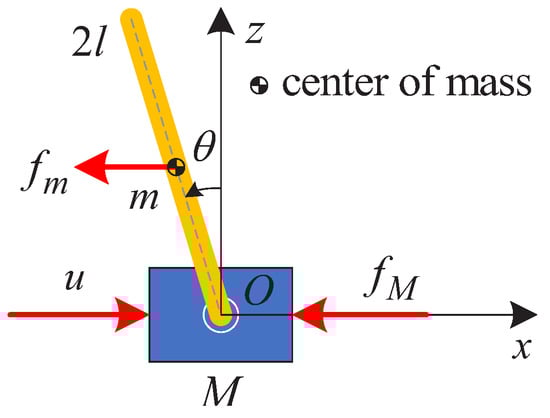
Figure 1.
The force analysis of the CIPS.
The junction point between the cart and the SIP is marked as the coordinate origin O. Under the actions of u and f, the cart moves in a straight line along the x-axis. Meanwhile, the SIP produces a pendulum motion on the plane with respect to the cart.
For the cart, the absolute coordinate of its center of mass is denoted as . Meanwhile, for the SIP, the absolute coordinate of its center of mass is denoted as . can be expressed as
The force analysis of the SIP is shown in Figure 2. In Figure 2, is the gravity (g is the gravitational acceleration). and are the forces exerted by the cart on the SIP along the x-axis and z-axis, respectively. According to the Euler equation, the resultant moment () of the SIP with respect to the coordinate origin (O) can be expressed as (2).
where is the angular acceleration of the SIP, and is the acceleration of the cart.
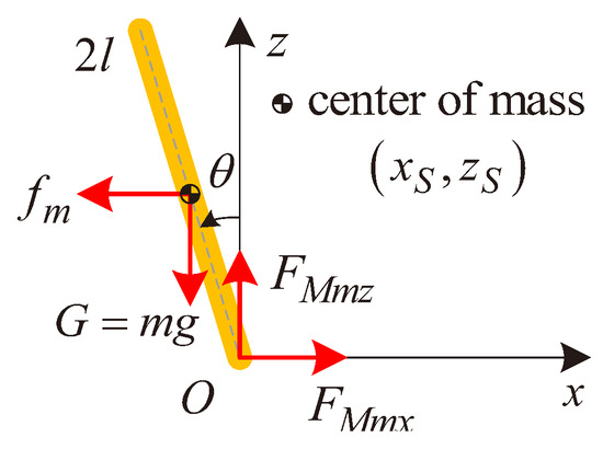
Figure 2.
The force analysis of the SIP.
For the SIP, the force analysis along the x-axis is shown in Figure 3. According to Newton’s second law of motion, it is easy to obtain that
where is the component of the acceleration of the SIP along the x-axis.
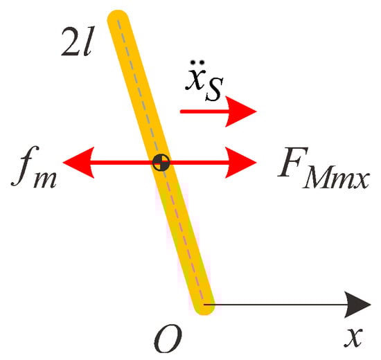
Figure 3.
The force analysis of the SIP along the x-axis.
Denoting as the force exerted by the SIP on the cart along the x-axis, according to Newton’s third law of motion, is expressed as
For the cart, the force analysis along the x-axis is shown in Figure 4. According to Newton’s second law of motion, it is easy to obtain that
where u is the driving force applied to the cart, which is also the control input of the whole CIPS. In addition, the friction force, f, can be calculated by
where is the friction factor, and is the velocity of the cart.
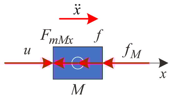
Figure 4.
The force analysis of the cart along the x-axis.
According to (1) and (4) to (6), it is easy to obtain that
where is the angular velocity of the SIP.
According to (2), is expressed as
The left side of the equals sign of (10) can be simplified as
2.2. Analyses of Motion Characteristics and Control Process
During the process of dynamic modeling, the friction force, f, the disturbance, , acting on the SIP, and the disturbance, , acting on the cart are considered, resulting in the dynamic Equation (14) of the CIPS complex. The complex dynamic Equation (14) brings great difficulty when it comes to analyzing the motion characteristics of the CIPS.
For the sake of simplicity, we employ the nominal dynamic equation of the CIPS to analyze its motion characteristics. When setting and in the dynamic Equation (14) of the CIPS, its nominal dynamic equation is obtained, i.e.,
where .
Let and ; under these conditions, the equilibrium points of the CIPS are obtained, i.e.,
where the equilibrium point represents the state where the cart is stationary at the x position of the x-axis and the SIP holds upright. The equilibrium point indicates that the cart is stationary at the x position of the x-axis, and the SIP is in a vertically downward position. In addition, is a stable equilibrium point of the CIPS, while is an unstable equilibrium point of the CIPS.
In this paper, the initial states of the CIPS are , i.e., the cart is stationary and the SIP is located in the upright position. The control objective of the CIPS is to control its states to reach the desired states , where denotes the desired position of the cart and denotes the desired states of the CIPS. In more detail, the control objective can be categorized as follows:
- (1)
- When the desired position is changed as a step setpoint, the cart can be controlled to reach this position, where is the maximum controllable motion range of the cart.
- (2)
- During the process of controlling the cart to track the desired position, , the SIP oscillates. When the cart reaches the desired position, , the pendulum angle of the SIP converges to zero, i.e., the SIP returns to the upright equilibrium point.
- (3)
- When considering the friction exerted to the cart, an impulse disturbance, , applied to the SIP, and an impulse disturbance applied to the cart, the above two control objectives can still be realized.
The above control objectives require stabilizing the SIP at the upright position, i.e., the CIPS is stabilized at one of its unstable equilibrium points. These control objectives are challenging. In addition, the dynamic Equation (14) of the CIPS has strong nonlinearity, which increases the difficulty of this control task.
3. Controller Design
To realize the control objectives (1) to (3) listed in the previous section, a gain-scheduled model predictive control method is proposed in this section. First, the dynamic Equation (14) of the CIPS is linearized at multiple different pendulum angles to obtain a series of linearized models, respectively. Second, a series of MPCs are designed based on these linearized models. Finally, one of these designed MPCs is selected to control the CIPS according to the gain schedule algorithm.
3.1. Linearization of Dynamic Equation
As shown in (14), the dynamic equation of the CIPS has strong nonlinearity. In addition, the control variable is the force, u, and the measurable output variables include the position, x, of the cart and the pendulum angle of the SIP. Since the MPC requires a linear time-invariant equation for executing the model prediction procedure, we first linearize the dynamic Equation (14) of the CIPS at a series of different pendulum angles to obtain various linearized models, respectively.
For any operating point, , on the trajectory of the dynamic Equation (14) of the CIPS, the following equations are satisfied:
For the ease of presentation, a variable, , is defined as
For any operating point, , on the trajectory of the dynamic Equation (17) of the CIPS, the following equations are satisfied:
Around the operating point, , the dynamic equation (Equation (17)) of the CIPS can be linearized as
where , , and are Jacobian matrices, where
where
In order to design the GSMPC, the dynamic Equation (14) of the CIPS is linearized at multiple different pendulum angles of to obtain n linearized models, respectively. For the ith linearized model , it can be obtained by setting in (22)–(25). In the next subsection, these n linearized models are employed as the prediction models to design the GSMPC.
3.2. Design of Gain-Scheduled MPC
In this subsection, a series of MPCs is first designed based on the linearized models obtained in the previous subsection. Then, a gain-schedule algorithm is proposed to switch among these designed MPCs for controlling the CIPS, based on the measured output pendulum angle of the SIP
In order to design the GSMPC, a series of single MPCs should be designed first. The block diagram of a single MPC is shown in Figure 5. According to [46], an MPC mainly consists of three parts, i.e., model prediction, rolling optimization, and feedback. The MPC enables the optimizer to determine the control strategy by solving the constrained finite-time optimal control problem. After computing the optimal control input sequence, only the first element of the control sequence is applied. In the next time step, the state of the system is measured, and a new constrained finite-time optimal control problem is solved on a rolling basis. This rolling time-domain control scheme introduces dynamic feedback into the system and is able to deal with modeling errors and uncertainties.
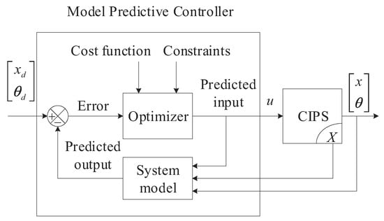
Figure 5.
The control system’s block diagram of the CIPS with a single MPC.
For a linear system, the MPC can be easily designed via MATLAB’s model predictive control toolbox. However, the dynamic Equation (14) or (17) of the CIPS represents a complex nonlinear system, which cannot be used directly to design the MPC. So, in this paper, the dynamic Equation (17) of the CIPS is linearized at a series of operating points, resulting in a series of linearized models. Each linearized model can be obtained according to (22)–(25). For each linearized model, an MPC can be easily designed via MATLAB’s model predictive control toolbox. Based on the above n linearized models, n MPC controllers are designed, respectively. The MPC corresponding to the ith linearized model is denoted as MPC-I .
Then, a gain-schedule algorithm is implemented to switch among these designed MPCs for controlling the CIPS, based on the measured output pendulum angle of the SIP. When the measured output pendulum angle of the SIP is closer to , the MPC-I is employed. Mathematically, the gain-schedule algorithm is expressed as
where is the distance between and . d denotes the set of . is the minimum value of all elements of d. j is the corresponding index of this minimum value.
According to the designed MPCs and the proposed gain-schedule algorithm, the GSMPC is designed. In this paper, we set to design the GSMPC. In addition, the control system block diagram of the CIPS is shown in Figure 6.
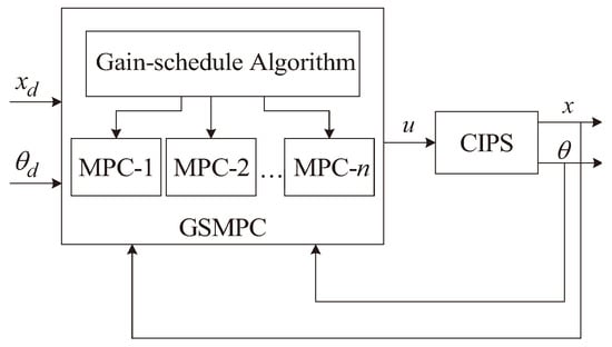
Figure 6.
The control system block diagram of the CIPS.
3.3. Stability Proof
The GSMPC consists of a series of single MPCs. The gain-schedule algorithm decides which single MPC is employed to control the CIPS during the control process. So, if the stability of all single MPCs can be proven, then the GSMPC is also stable.
For the MPC-I, the corresponding linearized model has the mathematical expression shown in (22). The continuous linearized model is transformed to the discrete form:
For each single linear MPC, the cost function is defined as (28) and the constraint is specified as
Then, the optimal problem can be formulated as
which is subjected to the following constraints:
where is the optimal control input sequence at the moment k.
The optimal problem (29) is solved by the optimizer, shown in Figure 5. According to the optimal solution, the optimal control input sequence and model predicted output at moment k are formulated as (31). In addition, the optimal value of at moment k is defined as , which can be computed according to (28).
Then, at moment , , and . So, the control input sequence can be selected as
According to (28), can be described as
So, is a feasible solution. The optimal solution is more superior than . According to (28) and (29), . According to (34), we can obtain
Therefore, the system is asymptotically stable no matter which single MPC is applied. So, the system is also asymptotically stable when applying the GMPC.
According to the above analysis, when the ith single MPC corresponding to the ith linearized model is applied, the control input applied to the CIPS is . So, for the GMPC, the control input applied to the CIPS is one element of set . According to the gain-schedule algorithm (26), the control input generated by the GSMPC is
4. Simulations
To demonstrate the validity and superiority of the proposed gain-scheduled model predictive control method, a series of simulations for the CIPS are conducted in MATLAB/Simulink. In the first set of simulations, pulse noise is used as the external disturbance, and four cases are considered for the simulations. In the second set of simulations, Gaussian white noise is employed as the external disturbance, with four cases also considered for these simulations.
4.1. Simulations I
In the first set of simulations, the parameters of the CIPS are listed in Table 1. In addition, the pulse noise is used as the external disturbance. Im particular, the following four cases are considered:

Table 1.
Parameters of the CIPS.
- Case (I–A): The CIPS is a nominal system, i.e., and in the simulation.
- Case (I–B): The SIP of the CIPS is subjected to a pulse disturbance with a magnitude of 2. As shown in Figure 7, for the ease of applying the pulse disturbance , the start time of is (s), the peak time of is (s), and the end time of is (s).
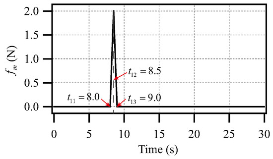 Figure 7. The pulse disturbance, , with a magnitude of 2 applied to the SIP of the CIPS.
 - Case (I–C): The cart of the CIPS is subjected to an impulse disturbance with a magnitude of 3. As shown in Figure 8, for the ease of applying the pulse disturbance , the start time of is (s), the peak time of is (s), and the end time of is (s).
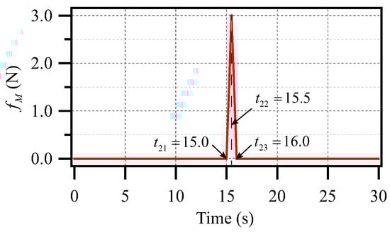 Figure 8. The pulse disturbance, , with a magnitude of 3 applied to the cart of the CIPS.
The desired position of the cart is set at and the desired pendulum angle of the SIP is set at . The simulation results from Case (I–A) to Case (I–D) are shown in Figure 9. The control inputs from Case (I–A) to Case (I–D) are shown in Figure 9e. For Case (I–A), the angle of the SIP converges to the desired pendulum angle (i.e., ) as the cart reaches the desired position (i.e., ). Moreover, both the angular velocity of the SIP and the velocity of the cart converge to zero, i.e., and . For Case (I–B), there is a jitter when the pulse disturbance (see Figure 7) is applied to the SIP. However, the designed GMPC can control the cart to reach the desired position and stabilize the SIP in the upright position. Moreover, both the angular velocity of the SIP and the velocity of the cart can converge to zero. For Case (I–C), there is a jitter when the pulse disturbance (see Figure 8) is applied to the cart. However, the designed GMPC can control the cart to reach the desired position and stabilize the SIP in the upright position and both the angular velocity of the SIP and the velocity of the cart can converge to zero. For Case (I–D), there are two jitters (see Figure 9). These two jitters occur when is applied to the SIP (see Figure 7) and applied to the cart (see Figure 8), respectively. However, even in this situation, the proposed GMPC can still control the CIPS to achieve the control objectives.
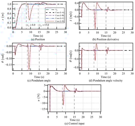
Figure 9.
Control results of the CIPS with pulse disturbances when .
When is increased to and the desired pendulum angle of the SIP is set at , the simulation results from Case (I–A) to Case (I–D) are shown in Figure 10. The control inputs from Case (I–A) to Case (I–D) are shown in Figure 10e. For Case (I–A), the angle of the SIP converges to the desired pendulum angle (i.e., ) as the cart reaches the desired position (i.e., ). Near (s), the above control objectives of the CIPS are reached. For Case (I–B), there is a jitter start from (s), which corresponds to the start time of the pulse disturbance . For Case (I–C), there is a jitter start from (s), which corresponds to the start time of the pulse disturbance . For Case (I–D), there are two jitters, which correspond to the application of the pulse disturbances and , respectively. From Figure 10, it can be observed that even when , the jitter occurring upon applying the pulse disturbance is larger than that resulting from applying the pulse disturbance . In addition, for Case (I–B), Case (I–C), and Case (I–D), the designed GMPC can regulate the CIPS to overcome the influences of the jitters and achieve the control objectives. These results indicate that using the proposed gain-scheduled model predictive control method, the SIP can be stabilized to the upright position while controlling the cart to reach a large desired position.
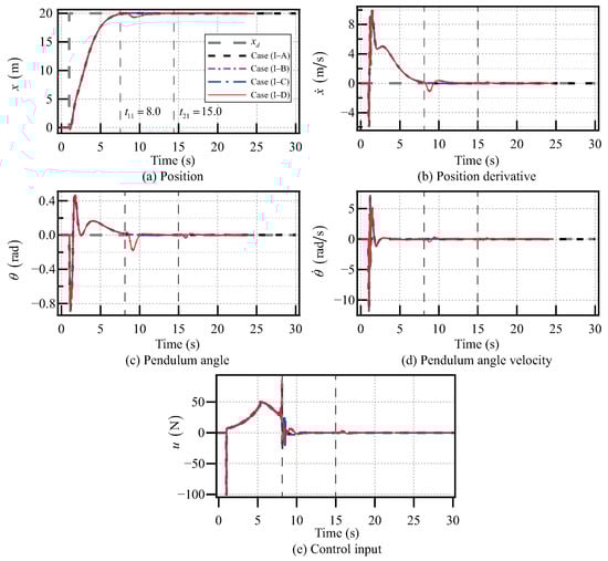
Figure 10.
Control results of the CIPS with pulse disturbances when .
Further, even when is increased to and and are exerted, the SIP can still return to its upright position and the cart is able to reach the desired position (as shown in Figure 11). So, within a large motion range of the cart, the control objectives of the CIPS can be reached with or without considering the disturbances. Thus, the proposed gain-scheduled model predictive control method for the CIPS is effective and superior.
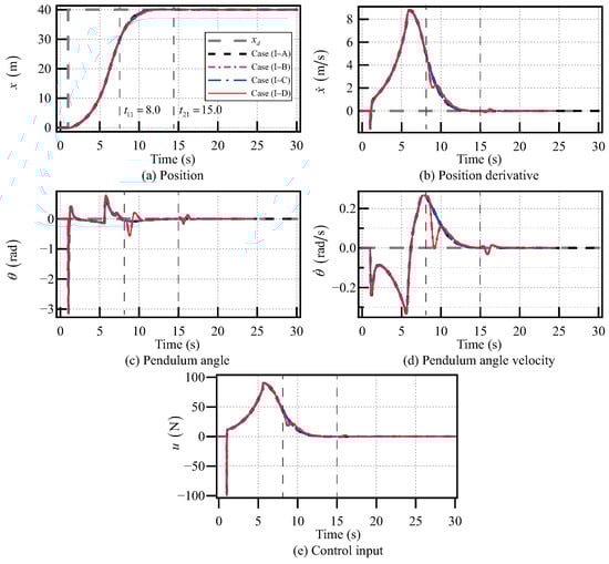
Figure 11.
Control results of the CIPS with pulse disturbances when .
4.2. Simulations II
In the second set of simulations, the parameters of the CIPS are also listed in Table 1. In addition, the Gaussian white noise is used as the external disturbance. Moreover, according to the applications of the disturbances and , the following four cases are considered.
- Case (II–A): The CIPS is a nominal system, i.e., and in the simulation.
- Case (II–B): The SIP of the CIPS is subjected to the disturbance, , in the form of Gaussian white noise. is shown in Figure 12.
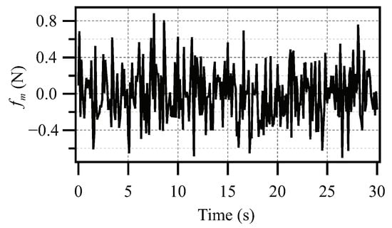 Figure 12. The Gaussian white noise, , applied to the SIP of the CIPS.
 - Case (II–C): The cart of the CIPS is subjected to the disturbance, , in the form of Gaussian white noise. is shown in Figure 13.
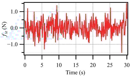 Figure 13. The white disturbance, , applied to the cart of the CIPS.
First, the desired position of the cart is set at and the desired pendulum angle of the SIP is set at . The simulation results from Case (II–A) to Case (II–D) are shown in Figure 14. The control inputs from Case (II–A) to Case (II–D) are shown in Figure 14e. For Case (II–A), the angle of the SIP is stabilized at the desired pendulum angle (i.e., ) while the cart reaches the desired position (i.e., ). Moreover, both the angular velocity of the SIP and the velocity of the cart converge to zero, i.e., and . From Case (II–B) to Case (II–D), the angle and angular velocity of the SIP, as well as the position x and the velocity of the cart exist disturbances. However, under the regulation of the proposed gain-scheduled model predictive control method, the angle of the SIP approaches zero and the position x of the cart approaches the desired position when reaching the stabilization phase of the CIPS. In addition, both the angular velocity of the SIP and the velocity of the cart approach zero.
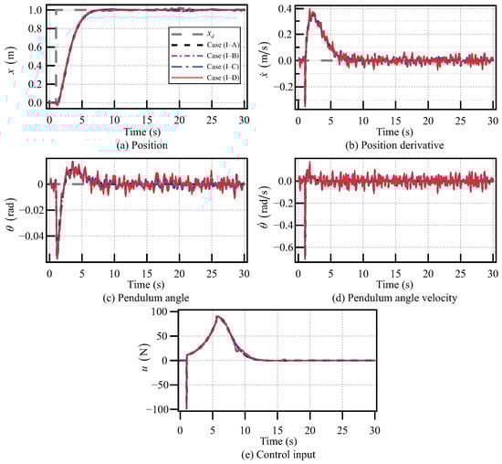
Figure 14.
Control results of the CIPS with Gaussian white noise disturbance when .
Then, the desired position of the cart is increased to , and the external disturbances and are set as Gaussian white noise. In addition, the desired pendulum angle of the SIP is set at . The simulation results from Case (II–A) to Case (II–D) are shown in Figure 15. The control inputs from Case (II–A) to Case (II–D) are shown in Figure 15e. From Figure 15, the angle of the SIP and the position x of the cart can be controlled to approach their desired values when applying the Gaussian white noise disturbance , or Gaussian white noise disturbance , or even both and . In addition, after entering the stabilization phase, both the angular velocity of the SIP and the velocity of the cart can be gradually controlled to approach zero. So, the proposed gain-scheduled model predictive control method works well when . Finally, even the desired position of the cart is increased to , the SIP can still return to the neighborhood of the upright position and the cart is able to reach the neighborhood of the desired position (as shown in Figure 16). So, within a large motion range of the cart, the control objectives of the CIPS can be reached with or without considering Gaussian white noise disturbances. Thus, the proposed gain-scheduled model predictive control method for the CIPS is efficacious and applicable.
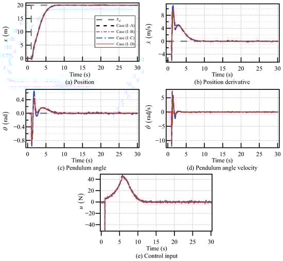
Figure 15.
Control results of the CIPS with Gaussian white noise disturbance when .
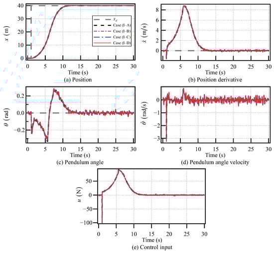
Figure 16.
Control results of the CIPS with Gaussian white noise disturbance when .
5. Conclusions
A gain-scheduled model predictive control method for the CIPS with friction and disturbances is proposed to control the cart’s movement to a new desired position. Meanwhile, during the motion process of the cart, the SIP returns to its upright position. Based on the Newton–Euler equation, the dynamic equation of the CIPS with friction and disturbances is given. According to the given dynamic equation of the CIPS, its motion characteristics and control process are analyzed. Then, the given dynamic equation of the CIPS is linearized to obtain a series of linearized models. Based on these linearized models, a series of MPCs are designed. In addition, a GSMPC is designed by proposing a gain-schedule algorithm to switch one of the designed MPCs to control the CIPS according to the measured output pendulum angle of the SIP. Finally, the effectiveness of the control strategy is verified by simulations.
The friction and disturbances have great influences on the control of the CIPS. When the friction and disturbances are not considered, the stabilization control of the CIPS can be realized smoothly. When considering the friction and disturbances, the jitters occur. However, the designed GMPC can regulate the CIPS to overcome the influences of the jitters and achieve the stabilization control objectives. When applying pulse disturbances and simultaneously, two jitters occur. After overcoming these two jitters by using the GMPC, both the SIP and cart of the CIPS can smoothly reach the desired position. When applying Gaussian white noise disturbances and simultaneously, the SIP has a slight oscillation near the upright position and the cart also has a slight vibration around its desired position. However, the position errors of the SIP and the cart are small, demonstrating that the stabilization control objectives of the CIPS can be realized by using the proposed gain-scheduled model predictive control method. In addition, the proposed control method has a wide range of applications in aerospace and robotics, such as balance control in robot walking, verticality control in rocket launching, and attitude control in satellite flight.
Author Contributions
Conceptualization, J.H.; methodology, J.H. and Y.L.; software, Z.W. and Z.H.; validation, J.H., Y.L., Z.W. and Z.H.; formal analysis, J.H. and Z.W.; investigation, Y.L. and Z.H.; resources, Z.H.; writing—original draft preparation, J.H. and Y.L.; project administration, Z.W.; funding acquisition, Z.H. All authors have read and agreed to the published version of the manuscript.
Funding
This work is supported by (1) Hubei Province Nature Science Foundation (no. 2023AFB380); (2) Hubei Key Laboratory of Digital Textile Equipment (Wuhan Textile University) (no. KDTL2022003); (3) Hubei Key Laboratory of Intelligent Robot (Wuhan Institute of Technology) (no. HBIRL202301).
Institutional Review Board Statement
Not applicable.
Informed Consent Statement
Not applicable.
Data Availability Statement
The data presented in this study are available on request from the corresponding author. The data are not publicly available due to privacy issues.
Conflicts of Interest
The authors declare no conflict of interest.
References
- Liu, Y.Y.; Slotine, J.J.; Barabási, A.L. Controllability of complex networks. Nature 2011, 473, 167–173. [Google Scholar] [CrossRef]
- Sankaranarayanan, V.; Mahindrakar, A.D. Control of a class of underactuated mechanical systems using sliding modes. IEEE Trans. Robot. 2009, 25, 459–467. [Google Scholar] [CrossRef]
- Odhner, L.U.; Jentoft, L.P.; Claffee, M.R.; Corson, N.; Tenzer, Y.; Ma, R.R.; Buehler, M.; Kohout, R.; Howe, R.D.; Dollar, A.M. A compliant, underactuated hand for robust manipulation. Int. J. Robot. Res. 2014, 33, 736–752. [Google Scholar] [CrossRef]
- Wang, L.; Lai, X.; Meng, Q.; Wu, M. Effective control method based on trajectory optimization for three-link vertical underactuated manipulators with only one active joint. IEEE Trans. Cybern. 2021, 53, 3782–3793. [Google Scholar] [CrossRef] [PubMed]
- Yang, T.; Chen, H.; Sun, N.; Fang, Y. Adaptive neural network output feedback control of uncertain underactuated systems with actuated and unactuated state constraints. IEEE Trans. Syst. Man Cybern. Syst. 2021, 52, 7027–7043. [Google Scholar] [CrossRef]
- Knoll, C.; Röbenack, K. Control of an underactuated manipulator using similarities to the double integrator. IFAC Proc. Vol. 2011, 44, 11501–11507. [Google Scholar] [CrossRef]
- Labrecque, P.D.; Laliberté, T.; Foucault, S.; Abdallah, M.E.; Gosselin, C. uMan: A low-impedance manipulator for human–robot cooperation based on underactuated redundancy. IEEE/ASME Trans. Mechatron. 2017, 22, 1401–1411. [Google Scholar] [CrossRef]
- Wang, L.; Lai, X.; Zhang, P.; Wu, M. A control strategy based on trajectory planning and optimization for two-link underactuated manipulators in vertical plane. IEEE Trans. Syst. Man Cybern. Syst. 2021, 52, 3466–3475. [Google Scholar] [CrossRef]
- Rigatos, G.; Siano, P.; Abbaszadeh, M. Nonlinear H-infinity control for 4-DOF underactuated overhead cranes. Trans. Inst. Meas. Control 2018, 40, 2364–2377. [Google Scholar] [CrossRef]
- Lee, H.W.; Roh, M.I.; Ham, S.H. Underactuated crane control for the automation of block erection in shipbuilding. Autom. Constr. 2021, 124, 103573. [Google Scholar] [CrossRef]
- Fu, Y.; Sun, N.; Yang, T.; Qiu, Z.; Fang, Y. Adaptive coupling anti-swing tracking control of underactuated dual boom crane systems. IEEE Trans. Syst. Man Cybern. Syst. 2021, 52, 4697–4709. [Google Scholar] [CrossRef]
- Pounds, P.E.; Dollar, A.M. Stability of helicopters in compliant contact under PD-PID control. IEEE Trans. Robot. 2014, 30, 1472–1486. [Google Scholar] [CrossRef]
- Karimoddini, A.; Lin, H.; Chen, B.M.; Lee, T.H. Hybrid three-dimensional formation control for unmanned helicopters. Automatica 2013, 49, 424–433. [Google Scholar] [CrossRef]
- Zhao, D.; Mishra, S.; Gandhi, F. A differential-flatness-based approach for autonomous helicopter shipboard landing. IEEE/ASME Trans. Mechatron. 2021, 27, 1557–1569. [Google Scholar]
- Greer, W.B.; Sultan, C. Infinite horizon model predictive control tracking application to helicopters. Aerosp. Sci. Technol. 2020, 98, 105675. [Google Scholar] [CrossRef]
- Marantos, P.; Bechlioulis, C.P.; Kyriakopoulos, K.J. Robust trajectory tracking control for small-scale unmanned helicopters with model uncertainties. IEEE Trans. Control Syst. Technol. 2017, 25, 2010–2021. [Google Scholar] [CrossRef]
- Shao, X.; Sun, G.; Yao, W.; Liu, J.; Wu, L. Adaptive sliding mode control for quadrotor UAVs with input saturation. IEEE/ASME Trans. Mechatron. 2022, 27, 1498–1509. [Google Scholar] [CrossRef]
- Ringbom, H.M.; Veal, R. Unmanned ships and the international regulatory framework. J. Int. Marit. Law 2017, 23, 100–118. [Google Scholar]
- Qu, Y.; Cai, L. Nonlinear positioning control for underactuated unmanned surface vehicles in the presence of environmental disturbances. IEEE/ASME Trans. Mechatron. 2022, 27, 5381–5391. [Google Scholar] [CrossRef]
- Chen, Y.; Chen, Y.; Chen, Y.; Zhao, H.; Mao, J.; Mao, J.; Chirarattananon, P.; Helbling, E.F.; Helbling, E.F.; Seung Patrick Hyun, N.; et al. Controlled flight of a microrobot powered by soft artificial muscles. Nature 2019, 575, 324–329. [Google Scholar] [CrossRef]
- Li, G.; Chen, X.; Zhou, F.; Liang, Y.; Xiao, Y.; Cao, X.; Zhang, Z.; Zhang, M.; Wu, B.; Yin, S.; et al. Self-powered soft robot in the Mariana Trench. Nature 2021, 591, 66–71. [Google Scholar] [CrossRef] [PubMed]
- Huang, X.; Zhu, X.; Gu, G. Kinematic modeling and characterization of soft parallel robots. IEEE Trans. Robot. 2022, 38, 3792–3806. [Google Scholar] [CrossRef]
- Ibanez, C.A.; Frias, O.G.; Castanon, M.S. Lyapunov-based controller for the inverted pendulum cart system. Nonlinear Dyn. 2005, 40, 367–374. [Google Scholar] [CrossRef]
- Maghzaoui, C.; Mansour, A.; Jerbi, H. A time-varying system control using implicit flatness: Case of an inverted pendulum. In Proceedings of the 2010 International Conference on Intelligent Systems, Modelling and Simulation, Liverpool, UK, 27–29 January 2010; pp. 276–281. [Google Scholar]
- Mondal, R.; Dey, J. Performance Analysis and Implementation of Fractional Order 2-DOF Control on Cart–Inverted Pendulum System. IEEE Trans. Ind. Appl. 2020, 56, 7055–7066. [Google Scholar] [CrossRef]
- Huang, Z.; Wei, S.; Hou, M.; Wang, L. Finite-time control strategy for swarm planar underactuated robots via motion planning and intelligent algorithm. Meas. Control 2023, 56, 813–819. [Google Scholar] [CrossRef]
- Sun, N.; Fang, Y. Nonlinear tracking control of underactuated cranes with load transferring and lowering: Theory and experimentation. Automatica 2014, 50, 2350–2357. [Google Scholar] [CrossRef]
- Muskinja, N.; Tovornik, B. Swinging up and stabilization of a real inverted pendulum. IEEE Trans. Ind. Electron. 2006, 53, 631–639. [Google Scholar] [CrossRef]
- Zhang, P.; Lai, X.; Wang, Y.; Su, C.Y.; Wu, M. A quick position control strategy based on optimization algorithm for a class of first-order nonholonomic system. Inf. Sci. 2018, 460, 264–278. [Google Scholar] [CrossRef]
- Taylor, J.R.; Taylor, J.R. Classical Mechanics; Springer: Berlin/Heidelberg, Germany, 2005. [Google Scholar]
- Santilli, R.M. Foundations of Theoretical Mechanics I: The Inverse Problem in Newtonian Mechanics; Springer Science & Business Media: Berlin/Heidelberg, Germany, 2013. [Google Scholar]
- Lanczos, C. The Variational Principles of Mechanics; Courier Corporation: Chelmsford, MA, USA, 2012. [Google Scholar]
- Jaafar, H.; Mohamed, Z.; Ahmad, M.; Wahab, N.; Ramli, L.; Shaheed, M. Control of an underactuated double-pendulum overhead crane using improved model reference command shaping: Design, simulation and experiment. Mech. Syst. Signal Process. 2021, 151, 107358. [Google Scholar] [CrossRef]
- Xu, R.; Özgüner, Ü. Sliding mode control of a class of underactuated systems. Automatica 2008, 44, 233–241. [Google Scholar] [CrossRef]
- Romero, J.G.; Donaire, A.; Ortega, R.; Borja, P. Global stabilisation of underactuated mechanical systems via PID passivity-based control. Automatica 2018, 96, 178–185. [Google Scholar] [CrossRef]
- Elmokadem, T.; Zribi, M.; Youcef-Toumi, K. Trajectory tracking sliding mode control of underactuated AUVs. Nonlinear Dyn. 2016, 84, 1079–1091. [Google Scholar] [CrossRef]
- Chen, X.; Zhao, H.; Sun, H.; Zhen, S.; Al Mamun, A. Optimal adaptive robust control based on cooperative game theory for a class of fuzzy underactuated mechanical systems. IEEE Trans. Cybern. 2020, 52, 3632–3644. [Google Scholar] [CrossRef]
- Li, H.; Yan, W.; Shi, Y. Continuous-time model predictive control of under-actuated spacecraft with bounded control torques. Automatica 2017, 75, 144–153. [Google Scholar] [CrossRef]
- Åström, K.J.; Hägglund, T. The future of PID control. Control Eng. Pract. 2001, 9, 1163–1175. [Google Scholar] [CrossRef]
- Garcia, C.E.; Prett, D.M.; Morari, M. Model predictive control: Theory and practice—A survey. Automatica 1989, 25, 335–348. [Google Scholar] [CrossRef]
- Morari, M.; Lee, J.H. Model predictive control: Past, present and future. Comput. Chem. Eng. 1999, 23, 667–682. [Google Scholar] [CrossRef]
- Holkar, K.; Waghmare, L.M. An overview of model predictive control. Int. J. Control Autom. 2010, 3, 47–63. [Google Scholar]
- Mayne, D.Q. Model predictive control: Recent developments and future promise. Automatica 2014, 50, 2967–2986. [Google Scholar] [CrossRef]
- Li, H.; Shi, Y. Event-triggered robust model predictive control of continuous-time nonlinear systems. Automatica 2014, 50, 1507–1513. [Google Scholar] [CrossRef]
- Messikh, L.; Guechi, E.H.; Blažič, S. Stabilization of the cart–inverted-pendulum system using state-feedback pole-independent MPC controllers. Sensors 2021, 22, 243. [Google Scholar] [CrossRef]
- Shen, C.; Shi, Y.; Buckham, B. Trajectory tracking control of an autonomous underwater vehicle using Lyapunov-based model predictive control. IEEE Trans. Ind. Electron. 2017, 65, 5796–5805. [Google Scholar] [CrossRef]
Disclaimer/Publisher’s Note: The statements, opinions and data contained in all publications are solely those of the individual author(s) and contributor(s) and not of MDPI and/or the editor(s). MDPI and/or the editor(s) disclaim responsibility for any injury to people or property resulting from any ideas, methods, instructions or products referred to in the content. |
© 2023 by the authors. Licensee MDPI, Basel, Switzerland. This article is an open access article distributed under the terms and conditions of the Creative Commons Attribution (CC BY) license (https://creativecommons.org/licenses/by/4.0/).