Article

Self-Improved Learning for Salient Object Detection

College of Computer Science and Technology, Zhejiang University, Hangzhou 310027, China
*
Author to whom correspondence should be addressed.
Appl. Sci. 2023, 13(23), 12966; https://doi.org/10.3390/app132312966
Submission received: 22 October 2023 / Revised: 28 November 2023 / Accepted: 30 November 2023 / Published: 4 December 2023
(This article belongs to the Special Issue Advances in Computer Vision and Semantic Segmentation)

Abstract

:
Salient Object Detection (SOD) aims at identifying the most visually distinctive objects in a scene. However, learning a mapping directly from a raw image to its corresponding saliency map is still challenging. First, the binary annotations of SOD impede the model from learning the mapping smoothly. Second, the annotator’s preference introduces noisy labeling in the SOD datasets. Motivated by these, we propose a novel learning framework which consists of the Self-Improvement Training (SIT) strategy and the Augmentation-based Consistent Learning (ACL) scheme. SIT aims at reducing the learning difficulty, which provides smooth labels and improves the SOD model in a momentum-updating manner. Meanwhile, ACL focuses on improving the robustness of models by regularizing the consistency between raw images and their corresponding augmented images. Extensive experiments on five challenging benchmark datasets demonstrate that the proposed framework can play a plug-and-play role in various existing state-of-the-art SOD methods and improve their performances on multiple benchmarks without any architecture modification.

1. Introduction

Salient Object Detection (SOD) refers to the problem of identifying the most visually distinctive objects. SOD methods typically learn a mapping from an image to a saliency mask, which benefits various downstream tasks such as object tracking [1], image captioning [2], video analysis [3], person re-identification [4], image retrieval [5], semantic segmentation [6], and object detection [7].
Despite the efforts long devoted to it, SOD remains a challenging task. One difficulty lies in the fact that the annotations are binary, i.e., each pixel is labeled either salient or non-salient, which does not fully capture the nuanced nature of saliency. For example, the four giraffes in Figure 1a are labeled as equally salient regardless of their different sizes, locations, and depths in the image. Furthermore, the binary annotations pose challenges in learning the mapping from images to saliency masks. The abrupt transition between salient and non-salient regions can make the learning process less smooth and hinder the ability of SOD models to generalize well to unseen data.
In this regard, we propose a novel Self-Improvement Training (SIT) strategy to reduce the learning difficulty incurred by the binary annotations. We design a progressively updated module to generate smooth labels, providing flexible degrees of saliency for each object to represent the difference of saliency between objects. The smooth labels provide more nuanced information about the saliency levels within an image, allowing the model to better understand the varying degrees of importance assigned to different objects. The use of smooth labels together with the binary annotations smoothens the learning process. However, it is worth noting that introducing smooth labels can also introduce noise into the training process. To this end, we mitigate the noise brought by the smooth labels by adapting the weights of smooth labels in the optimization phase.
Another difficulty is that the annotations are subjective, i.e., the saliency of an object is influenced by the annotator’s personal preference. As shown in Figure 1b, the hollow part of a bicycle is labeled salient in the left but not salient in the right. Moreover, both images with butterflies in Figure 1b share similar layouts (butterfly, flowers, and green background) but the flowers are marked as salient in the left image and not salient in the right. Therefore, SOD requires the model to be of high robustness to noisy labeling.
To improve the robustness, we propose a novel Augmentation-based Consistent Learning (ACL) scheme. By simulating a cross-dataset validation scenario, ACL introduces salient-related data augmentation to images, aiming to enhance the consistency of predictions between raw and augmented images. In this way, ACL makes the prediction of a raw image be consistent to that of the augmented image. As a result, the SOD model is capable of accurately locating the most salient objects while disregarding irrelevant variations caused by augmentation, thus improving the robustness of the model.
Our main contributions are summarized as follows.
  • We propose a novel Self-Improved Training strategy for SOD, which reduces the learning difficulty and effectively improves the performance.
  • We present an Augmentation-based Consistent Learning scheme that regularizes the consistency between raw images and their corresponding augmented images at training time and improves the robustness of the models.
  • The proposed method is model independent, which can be applied to existing prevalent methods without modifying the architecture to gain considerable improvements.

2. Related Work

2.1. Network Designs for SOD

The network designs for Salient Object Detection can be summarized into three categories: architecture-based, aggregation-based, and contour-based methods.
First, architecture-based methods explore various feature extractors for SOD. Early methods such as [11,12,13,14,15,16,17] obtain handcrafted or deep features from image subunits and use MLP classifiers to predict saliency scores based on the features. For example, SuperCNN [16] and Multi-Context [13] use super-pixels or patches as image subunits. These methods fail to model the global context and cannot be trained end to end. Inspired by FCNs [18], CNN-based methods [19,20,21,22,23,24,25] formulate the salient object detection as a pixel-level prediction task and generate the saliency map in an end-to-end manner. Recently, Transformer has also been applied to SOD [26,27,28,29,30]. They combine both Transformer and CNN to process multi-level features. For instance, VST [30] considers the SOD task from the sequence-to-sequence perspective and designs a pure transformer model to handle the tokenized input. In addition, Transformer is also utilized to model the cross-modal information from the RGB and depth data [26,27].
Second, aggregation-based methods focus on feature aggregation or feature fusion to combine features from different layers. These methods capture both spatial details and global semantics for an accurate saliency map [13,24,31,32,33,34,35,36]. A simple yet effective way is to skip connect the features from the encoder to the features with the same spatial size from the decoder. This U-shape-based structure has been employed in many works [13,35,36]. Furthermore, GateNet [34] introduces gated mechanisms to control the information fusion flow. Also, channel-wise attention and spatial-wise attention have been applied to weigh the importance during the feature aggregation process [31,32,33]. MENet [37] designs a multi-scale feature enhancement module to gradually aggregate and refine global or detailed features by changing the size order of the input feature sequence.
To achieve high-quality saliency prediction with fine edge details, contour-based methods attempt to explicitly regularize the contours of salient objects. This line of work involves two aspects: network design and loss function design. Contour-aware networks attempt to model contours explicitly [32,33,38,39]. Specifically, EGNet [38] proposes to make the model predict saliency and contours simultaneously. Based on this, C2SNet [39] adopts an alternating converting method between contour maps and saliency maps. Unlike existing two-branch methods [33,38] that use one branch for the boundary and the other one for the entire object, MENet [37] uses two parallel branches that learn internal regional features and global features, respectively, so as to reduce the interference of inaccurate boundary information with global features. Some other works design contour-aware loss functions. The structural similarity index (SSIM) [40] and weighted BCE loss [41] are introduced for more edge details in the saliency maps.
Our method aims to smoothen the learning process and improve the robustness of SOD. We do not design a specific architecture or model contours for SOD explicitly. Instead, our learning strategy is capable of working with all these methods without modifying their networks.

2.2. Non-Fully Supervised Learning for SOD

To alleviate the burden of human efforts on pixel-level annotations, semi-/weakly-supervised methods for SOD have been proposed. These methods require image-level [42,43,44,45,46], scribble-level [47,48], or point-level annotations [49,50]. For example, FIN [42] leverages the category labels and is jointly optimized with an FCN to capture potentially salient regions. WS3A [47] uses scribbles annotation to do local supervision while utilizing auxiliary edges to provide details. PSOD [49] uses point annotation to provide the locations of salient objects to obtain pseudo labels to gain the first round of supervision, and then again uses point annotation to suppress non-salient objects to obtain optimized pseudo labels for the second round.
Recent years also witness the adoption of self-supervised learning for SOD, which requires no human annotations. A2S [51] and A2Sv2 [52] employ large-scale unsupervised pre-trained networks. They utilize a two-step approach where the first stage involves constructing reliable pseudo labels and the second stage trains the final segmenter after intermediate label processing. UNSS [53] introduces a top–down context guidance strategy that extracts detailed signals for both global and local segmentation learning.
In this paper, the training of our method consists of two parts: the Self-Improvement Training strategy (SIT) and Augmentation-based Consistent Learning. They are motivated by self-supervised learning, but both of them utilize pixel-level annotations. Specifically, SIT utilizes the SOD model, which uses pixel-level annotations, to generate smooth labels to alleviate the training difficulty of itself. ACL adopts the CutOut augmentation to remove part of the image and forces the model to make the results of the augmented image consistent with the results of the original image. The removed part is determined using the ground truth, and thus, ACL cannot be treated as unsupervised. In essence, the aim of ACL is to make the model robust instead of reducing human efforts on annotations.

3. Method

Salient object detection learns a function from an image to saliency predictions. Generally, an SOD network F SOD consists of an encoder E and a decoder D. Given an input RGB image x R H × W × 3 and its ground truth y { 0 , 1 } H × W with the height H and width W, encoder E extracts features and decoder D generates a saliency prediction p R H × W by p = F SOD ( x ) = D ( E ( x ) ) .
Next, we present our framework as illustrated in Figure 2a. We design the proposed Self-Improvement Training strategy (SIT) in Section 3.1 and Augmentation-based Consistent Learning scheme (ACL) in Section 3.2. Finally, we summarize the whole training procedure in Section 3.3.

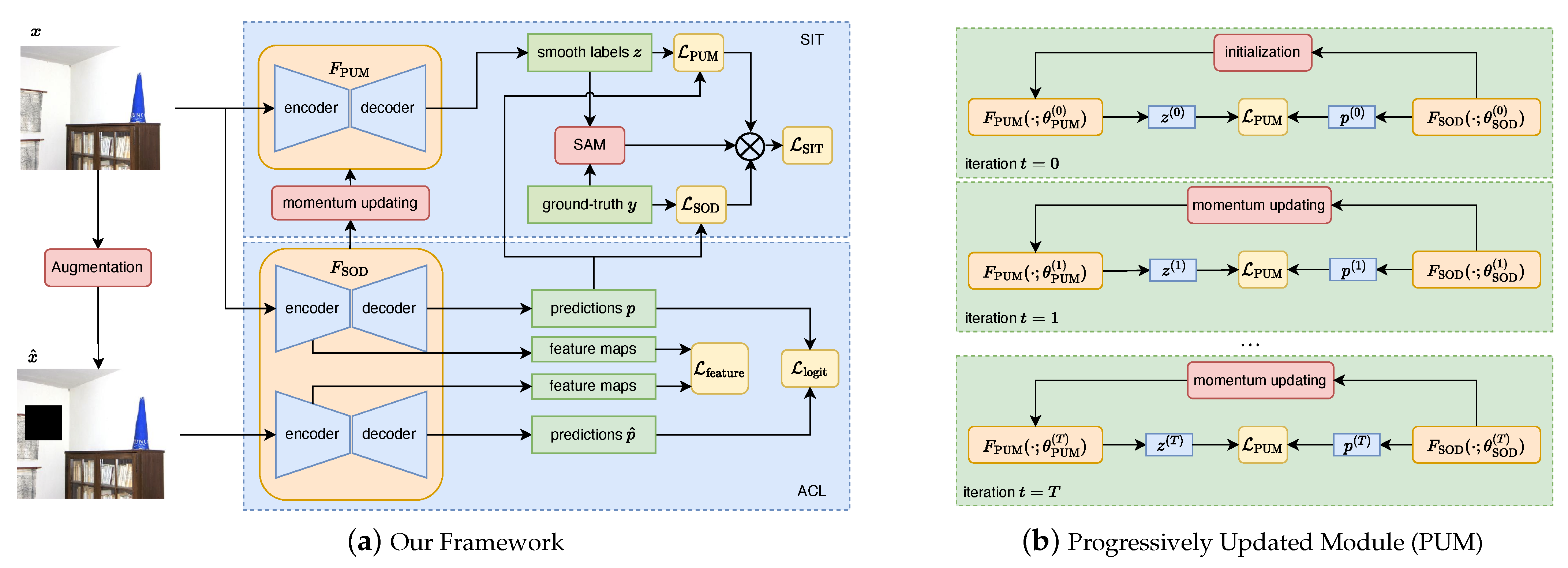
3.1. Self-Improvement Training Strategy

In this work, we propose a Self-Improvement Training (SIT) strategy to reduce the learning difficulty by relaxing the binary annotations with smooth labels. We decompose SIT into two steps. First, we generate smooth labels with a proposed Progressively Updated Module (PUM). Second, we design a Sample Adaptive Module (SAM) to weigh the balance between binary and smooth labels.

3.1.1. PUM: Progressively Updated Module

Formally, we design a progressively updated module (PUM), denoted by F PUM , to generate smooth labels. F PUM shares the same network structure with the SOD network F SOD . Specifically, let the parameters of F SOD be θ SOD , and the parameters of F PUM be θ PUM . First, we randomly initialize θ SOD . Then, we initialize θ PUM by
t = 0 : θ PUM ( 0 ) = θ SOD ( 0 ) ,
where t is the iteration of the training (Iteration t refers to a mini-batch training iteration instead of an epoch). At this point, F PUM is identical to F SOD . They can only generate a random salient output before training. To progressively improve the quality of the smooth labels, we update θ PUM at a momentum coefficient η from θ SOD as follows
t = 1 : θ PUM ( 1 ) = η · θ PUM ( 0 ) + ( 1 η ) · θ SOD ( 1 ) , t = 2 : θ PUM ( 2 ) = η · θ PUM ( 1 ) + ( 1 η ) · θ SOD ( 2 ) , t = T : θ PUM ( T ) = η · θ PUM ( T 1 ) + ( 1 η ) · θ SOD ( T ) .
It is worth noting that only parameters θ SOD are updated via backpropagation, whereas parameters θ PUM are updated progressively by θ SOD at the training time of F SOD . The momentum update in Equation (2) makes θ PUM evolve more smoothly than θ SOD . As a result, the generated smooth labels are improved smoothly with the training of F SOD . In this way, the PUM progressively integrates the parameter from the SOD network and generates more informative supervisions for the output of the SOD network during training, as illustrated in Figure 2b.
With PUM, we can obtain smooth labels z by feeding an input image x into F PUM as
z ( t ) = F PUM ( x ; θ PUM ( t ) ) ,
where predictions z are of the same size as ground truth y. While y is { 0 , 1 } H × W , z is ( 0 , 1 ] H × W
With smooth labels z, we regularize F SOD by
L PUM = i = 1 H j = 1 W ( p i , j ( t ) z i , j ( t ) ) 2 ,
where p ( 0 , 1 ] H × W are the predictions of F SOD , and z ( 0 , 1 ] H × W are the obtained smooth labels by F PUM .

3.1.2. SAM: Sample Adaptive Module

Although smooth labels z aim at providing more informative supervisions for the output of the SOD network, they are noisy and unreliable at the beginning of the training. Figure 3 shows that the quality of the smooth labels is getting better and better as the training goes. To alleviate the noise incurred by smooth labels z, we introduce an adaptive weight λ defined by
λ = exp ( ζ · ( y · log z ( t ) + ( 1 y ) · log ( 1 z ( t ) ) ) ) ,
where y is the ground truth, z ( t ) are the smooth labels at training iteration t, and ζ is a hyperparameter. The definition of λ implies that λ is always positive, and that when z is significantly different from y, which means the quality of the smooth labels is bad, λ will be close to zero. In this way, instead of directly enforcing F SOD to mimic the output from F PUM , our Sample Adaptive Module (SAM) measures the quality of generated smooth labels and strikes a balance between ground truth and the smooth labels. As a result, the overall loss function of SIT is
L SIT = L SOD + λ · L PUM ,
where L PUM is defined in Equation (4), and L SOD is the commonly used SOD loss function defined by
L SOD = i = 1 H j = 1 W ( y i , j · log p i , j + ( 1 y i , j ) · log ( 1 p i , j ) ) .
At the beginning of training, z is noisy, which leads to a very small λ to punish the impact of L PUM . As the training goes, the quality of z will be better and better and λ will be larger, which makes the impact of L PUM more significant. In other words, as the quality of smooth labels becomes better, F SOD will learn more from F PUM .

3.2. Augmentation-Based Consistent Learning

We design an augmentation-based consistent learning (ACL) scheme to keep the model’s robustness for the salient-related data augmentation. By regularizing the model at both the prediction level and feature level, ACL helps the SOD model to capture more discriminative contextual information and improve the robustness.

3.2.1. Regularizing with Prediction Consistency

We first augment the raw image x with task-specific augmentation methods (detailed in Section 4.1.3) and obtain its augmentations x ^ and its corresponding saliency prediction p ^ . Next, we regularize the prediction consistency between the raw image and its augmentations by
L logit = i = 1 H j = 1 W ( p i , j ( t ) p ^ i , j ( t ) ) 2 ,
where p is the prediction of x and p ^ is the prediction of x ^ .

3.2.2. Regularizing with Feature Consistency

Moreover, we introduce a multiscale feature consistency loss L feature to regularize the feature consistency for each layer of encoder E i between the raw image x and augmented image x ^ by
L feature = i = 1 N E i ( x ; θ SOD ( t ) ) E i ( x ^ ; θ SOD ( t ) ) F 2 ,
where N is the number of feature levels in encoder E, E i ( x ) are the features of x at the i-th layer of E, E i ( x ^ ) are the features of x ^ at the i-th layer, and · F is the Frobenius norm of the matrix.

3.3. The Training Procedure

Finally, we put all things together and train F SOD in an end-to-end manner. The total loss L total is defined as
L total = L SIT + L logit + L feature .
The optimization procedure of our proposed method is summarized in Algorithm 1. It is worth noting that our method is orthogonal to the network architectures; thus, it can work as a plug-and-play module to boost the existing methods.
Algorithm 1 SIT and ACL training strategy at the t iteration
Input: x, an input images; y, its ground-truth
Networks:  F SOD ( · ; θ SOD ) , an SOD network with its parameters; F PUM ( · ; θ PUM ) , a PUM network with its parameters
Output:  θ SOD , θ PUM .
  1:
Initialization: θ PUM ( 0 ) θ SOD ( 0 )
  2:
for t = 1  to  T  do
    // SIT Self-Improvement Training Strategy
  3:
     p = F SOD ( x ; θ SOD ( t 1 ) ) // Obtain saliency prediction
  4:
     z = F PUM ( x ; θ PUM ( t 1 ) ) // Obtain smooth label
  5:
    Compute the SIT loss L SIT defined in Equation (6)
 
     / /  ACL Augmentation-based Consistent Learning
  6:
     x ^ = Augment ( x )   / /  Get augmentation
  7:
     p ^ = F SOD ( x ^ ; θ SOD ( t 1 ) ) // Obtain saliency prediction
  8:
    Compute L logit and L feature // defined in Equations (8) and (9)
 
     / / Network Optimization
  9:
    Compute the total loss L total defined in Equation (10)
 10:
     θ SOD ( t ) Adam ( L total , θ SOD ( t 1 ) ) // Optimize SOD network
 11:
     θ PUM ( t ) η · θ PUM ( t 1 ) + ( 1 η ) · θ SOD ( t ) // Update PUM
 12:
end for
 13:
return θ SOD , θ PUM

4. Experiment

In this section, we evaluate our method. First, we describe the experiment setup in Section 4.1. Next, we conduct a series of ablation studies to demonstrate the impact of each component in our proposed framework and compare our method with others in Section 4.2. Furthermore, we carry out a detailed analysis of different design choices of our proposed SIT and ACL in Section 4.3. Finally, we present a visual comparison in Section 4.4.

4.1. Experiment Setup

4.1.1. Datasets

We evaluate our method on five popular datasets as shown in Table 1, including ECSSD [10] with 1000 images, PASCAL-S [8] with 850 images, DUT-OMRON [9] with 5168 images, HKU-IS [11] with 4447 images, and DUTS [42] with 15,572 images. All datasets are human-labeled with pixel-wise ground truth for quantitative evaluations. DUTS is currently the largest SOD dataset, which is divided into 10,553 training images (DUTS-TR) and 5019 testing images (DUTS-TE). We follow [40,54] to use DUTS-TR as the training dataset and the others as the testing datasets.

4.1.2. Evaluation Metrics

For all the experiments, we use four evaluation metrics to measure the performance, including the Mean Absolute Error (MAE), Mean F-measure ( m F ), structural similarity measure ( S α , α = 0.5 ) [55], and E-measure ( E ξ ) [56].
First, MAE is a metric that computes the average absolute difference between the predicted saliency map p and its corresponding ground-truth map y pixel-by-pixel as follows
M A E = 1 H × W i = 1 H j = 1 W | p i , j y i , j | ,
where H and W are the height and width of p correspondingly. Second, the F-measure, termed m F , is a metric that evaluates both precision and recall comprehensively, and we provide the mean F-measure using varying fixed (0–255) thresholds. Next, the S-measure, termed S α , is a metric that consists of the region-aware ( S r ) and object-aware ( S o ) structural similarity:
S α = α · S o + ( 1 α ) · S r ,
where α is set to 0.5 to weigh the balance. Finally, the E-measure, termed E ξ , is a metric that takes both the image-level mean value and local pixel matching information into consideration to evaluate the similarity between the prediction and the ground truth.

4.1.3. Implementation Details

Our framework is implemented via PyTorch. As our goal is to design a general model independent framework, we choose three state-of-the-art SOD algorithms: F 3 Net [57], MINet [58], and GateNet [34] as baselines and integrate our methods into these different baselines. ResNet-50 [59], pre-trained on ImageNet, is used as the backbone network for all the three baselines. For training the hyperparameters’ setting, we follow different baseline’s implementation details according to their paper. For the data augmentation method in ACL, we use CutOut [60]. Specifically, we will conduct Cutout on the image area where there are no salient objects.

4.2. Ablation Study

First, we carry out ablation experiments to validate the effectiveness of our proposed SIT strategy and ACL scheme. Then, we integrate the proposed framework into different SOD baseline models. Since our method is orthogonal to the network architectures, we conduct all ablation studies on the basis of F 3 Net due to its flexibility and effectiveness without a loss of generality.

4.2.1. Effectiveness of SIT

The integration of SIT (the second row in Table 2) gives performance gains of 0.7%, 0.3%, and 0.2%, in terms of m F , S α , and E ξ on the DUTS-TE dataset over the F 3 Net baseline, respectively. Such results validate that the SIT strategy serves as a useful way to reduce the learning difficulty and improve the performance.

4.2.2. Effectiveness of ACL

As shown in the third row of Table 2, simply embedding the ACL scheme into the F 3 Net baseline also helps improve the performance on both m F and E ξ on the DUTS-TE dataset by 0.5% and 0.3%, respectively. It reveals that the robustness of the model is improved by enforcing consistency regularization for augmented images in ACL. The visual effects of ACL are illustrated in Figure 4. We can see that ACL helps effectively suppress the distracting background and accurately locate the salient objects because the richer contextual information can be captured via the consistency learning process.

4.2.3. The Whole Framework

To demonstrate the effectiveness of the proposed methods, we compare it against 13 state-of-the-art SOD algorithms, including AFNet [33], BASNet [40], CPD-R [54], BMPM [24], R 3 Net [61], PiCA-R [23], DGRL [22], TDBU [62], PoolNet [63], PAGE [32], RAS [64], C2SNet [39], and F 3 Net [57]. As shown in Table 3, the performances of these baselines are boosted considerably by being integrated with our proposed framework.
Compared with the baselines, the m F results of our method on the DUTS-TE dataset are improved by 0.6%, 0.6%, and 0.2% based on three different baselines, respectively. In addition, Figure 5 shows the standard PR curves and the F-measure curves of the aforementioned baselines on the DUTS dataset, which can evaluate the performance of the models comprehensively. From these curves, we can observe that the models trained with our framework consistently outperform all corresponding baselines under different thresholds, which means that our framework has an excellent capability to detect salient regions and generate accurate saliency maps. All of these reveal that the proposed framework is effective on different SOTA methods and achieves a clearly better-averaged performance gain without modifying any architecture.

4.3. Analysis on Design Choices

We analyze the design choices of our method from three aspects. First, we explore the updating strategy of PUM. Second, we conduct an ablation study of the selection of momentum coefficient. Finally, we show the effectiveness of the proposed SAM.

4.3.1. Updating Strategy of PUM

To obtained smooth labels in SIT, we need to update the PUM module from the SOD network. A straightforward updating strategy is to update the PUM module only once per epoch, which is similar to the Π model [65]. In this paper, we adopt a momentum-updating manner to integrate models of different steps to the PUM module progressively. From Table 4, we can see that all the momentum-updating strategy settings outperform the epoch-based updating strategy setting. With the momentum coefficient η in the range of 0.9 to 0.9999, the momentum-updating strategy could achieve a stable performance improvement, exceeding the epoch-based updating strategy on average by 1.1% on m F and 0.8% in S α .

4.3.2. The Selection of Momentum Coefficient η

As described in Section 3.1, the momentum coefficient η determines the update speed of θ PUM . Our model’s sensitivity to η is shown in Table 4. When η is set to 0.99, the model can achieve the best performance on all metrics. We have revised this part to present our results more clearly.

4.3.3. Effect of Sample Adaptive Module

In this Sample Adaptive Module (SAM), we introduce an adaptive weight to dynamically tune the loss contribution between ground truth and smooth labels. To demonstrate the effectiveness of our SAM, we compared our dynamic adaptive weight strategy with a fixed weight strategy. We choose three different fixed weights, which are 0.3, 0.5, and 0.7, respectively. From Table 5, we can observe that our SAM method exceeds all the fixed weight settings. Compared with the best fixed weight setting ( λ = 0.3), the m F of our SAM method exceeds it by 0.5%, which illustrates the effectiveness of SAM.
The hyperparameter ζ in Equation (5) is used to modulate the loss contribution of the PUM module. Thus, we conduct a series of experiments to evaluate the effect of hyperparameter ζ . As shown in Table 6, setting ζ to 70 makes the model learn well from the PUM module and obtain the best performance with 0.846 on m F .

4.4. Visualization Analysis

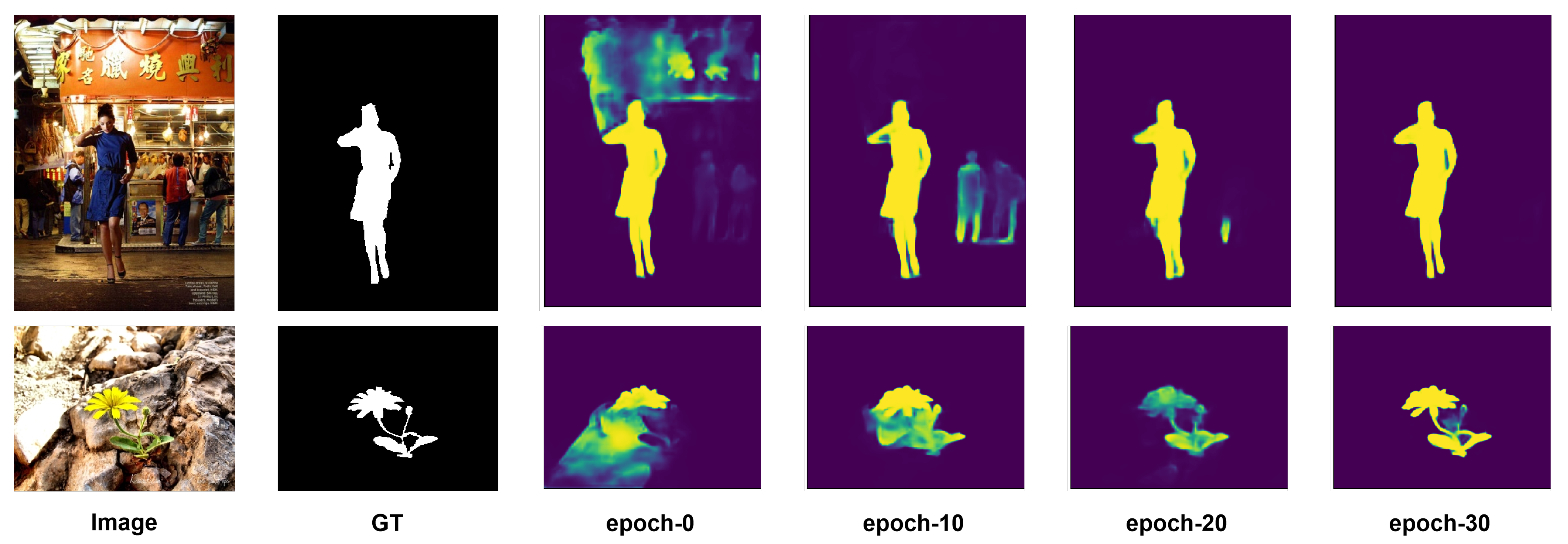
4.4.1. Visualization of Smooth Labels

In this part, we show the smooth labels generated via the PUM at different training iterations. As shown in Figure 3, we can observe that the PUM gradually improves the quality of the smooth labels. As the learning process progresses, the smooth labels not only obtain a sharper boundary but also suppress the distractors in the background.

4.4.2. Visualization of Feature Attention Maps

To further demonstrate the effectiveness of our framework, we visualize some attention maps in Figure 6. It can be observed that even if the squirrel has very low contrast with the ground (see the second column), by using our framework, the high contrast between the object region and the background is always maintained, thereby making the salient objects be effectively distinguished. In addition, our framework can effectively suppress distraction objects (see the fifth column). The people in the corner of the image are suppressed well in the feature attention map.

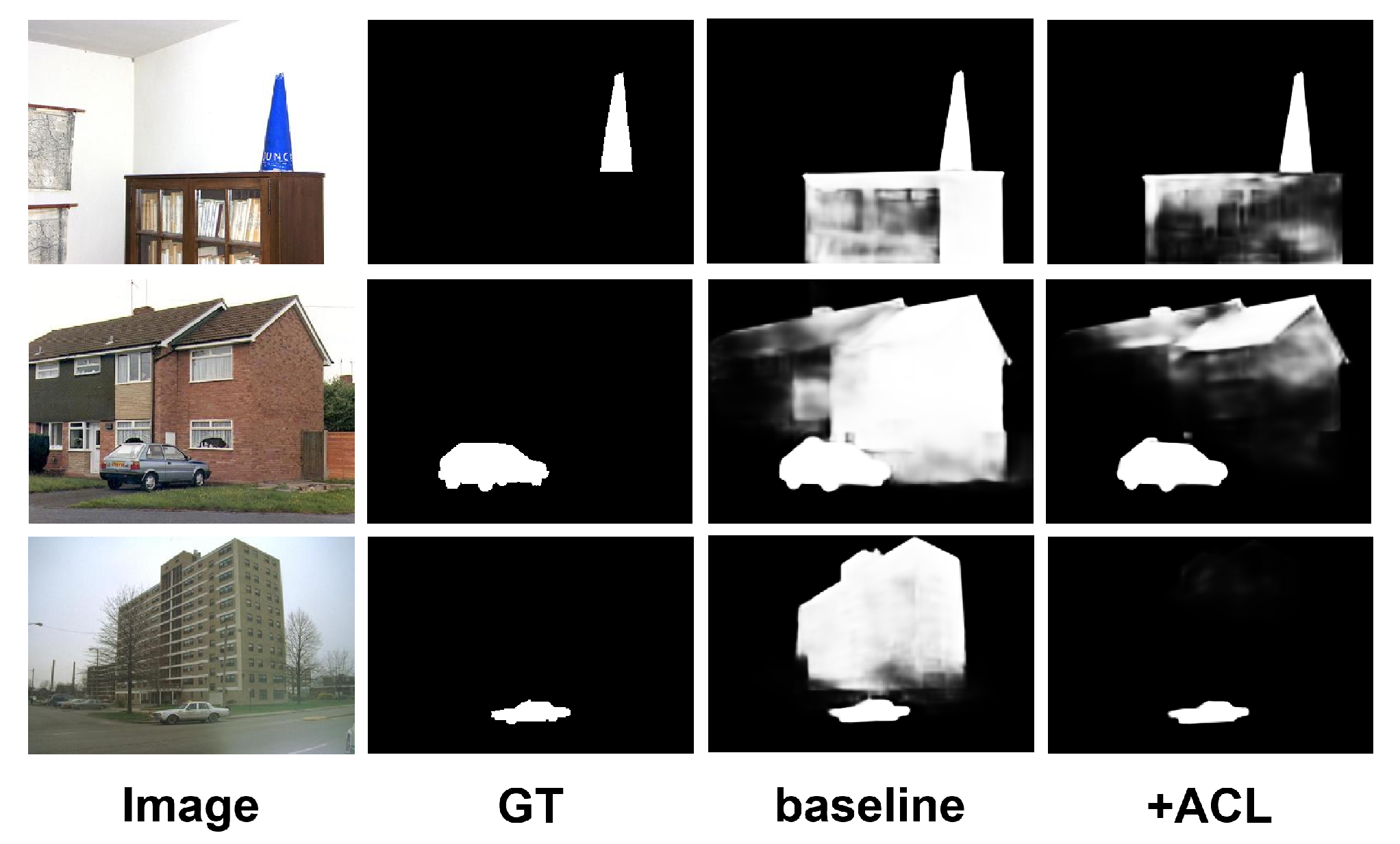
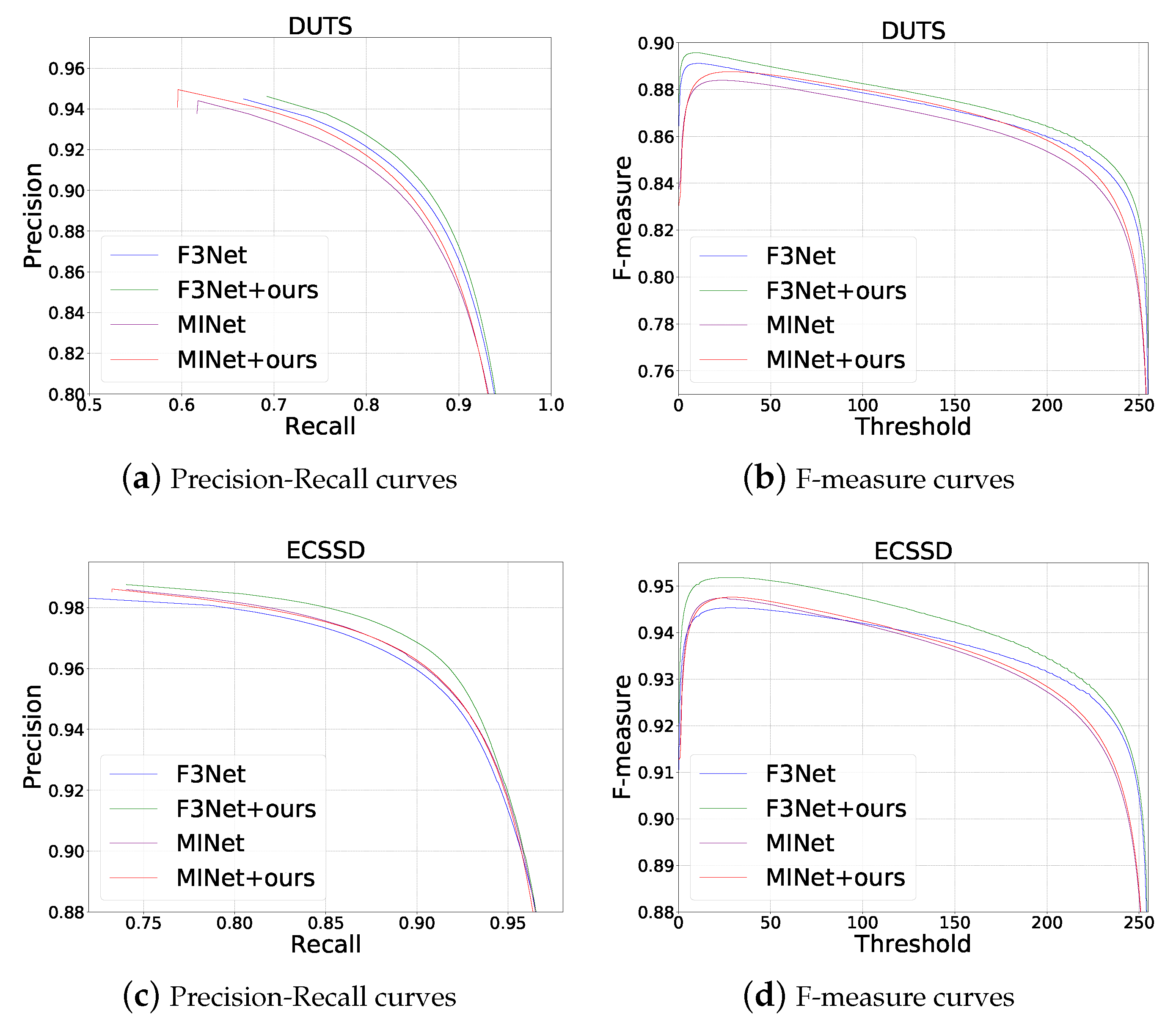
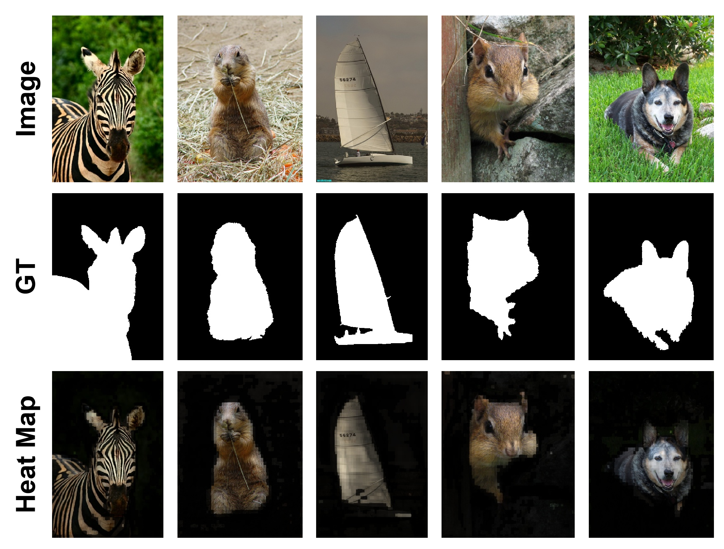
4.4.3. Visual Comparison with Baseline Methods

To evaluate the robustness and effectiveness of our framework, we visualize some saliency maps and exhibit some typical images from the public test dataset of saliency detection in Figure 7.
In the first, second, and fifth rows, the complex backgrounds. such as seats and windows in the first row, stacked boxes in the second row, and books in the fifth row, are suppressed in ours but highlighted in all other baselines. Especially for the first and second rows, the backgrounds are suppressed well. Presumably, it is because the color of these backgrounds’ objects are similar. Thus, our method can accurately locate and suppress all of them. In the third row, the baseline methods are severely affected by the gray box. Our framework can not only better pick out the salient objects accurately, but it also well suppresses these distractors. In the fourth and sixth row, the baseline methods fail to capture complete salient objects, such as the person on the left in the fourth row and the elephant on the right in the sixth row. However, our framework can accurately locate these salient objects.
In a word, our proposed framework can possess good robustness and effectiveness in detecting various salient objects.

4.5. Discussion

In this part, we will discuss the strengths and weaknesses of our method. Let us review the visual comparison in Figure 6. The third column shows a sailing boat. Our method misses its hull. The fourth column is a squirrel. Our method misses its paw. The fifth column is a dog. Our method misses its forelegs. These errors have a common point: the method misses their spatial details.
That being said, our method can predict results with spatial details as shown in the first row of Figure 7. In this case, all of our models (F 3 Net+ours, MINet+ours, and GateNet+ours) can detect the contour of the person’s feet. However, by looking at the pictures more carefully, one can find that the detection of the foot’s contour should be attributed to the baseline models (F 3 Net, MINet, and GateNet). F 3 Net+ours has a similar foot’s contour as F 3 Net. Similar results can be found in MINet vs. MINet+ours and GateNet vs. GateNet+ours.
Our method aims to alleviate the learning difficulty and improve the robustness of the SOD methods. We do not design specific contour-based techniques to improve the performance, but these techniques are orthogonal and complementary to our work.

5. Conclusions

In this paper, we present a learning framework to reduce the learning difficulty for the SOD task. A novel self-improvement training (SIT) strategy is designed to generate smooth labels, which alleviates the learning difficulty. Moreover, by regularizing the prediction consistency and multi-level feature consistency in augmentation-based consistent learning (ACL), the robustness of the model can be further improved. Comprehensive benchmarks on several popular datasets illustrate the advantage of the proposed framework. A further ablation study shows the effectiveness of each method of our framework. Briefly, our framework can play a plug-and-play role to be easily embedded in the existing SOD networks to achieve a promising performance gain, without any modification of the network architecture.

Author Contributions

Conceptualization, S.L. and H.W.; methodology, S.L. and H.W.; software, H.Z.; writing—original draft, S.L. and H.Z.; writing—review and editing S.L.; supervision, X.L.; project administration, S.L. All authors have read and agreed to the published version of the manuscript.

Funding

This research received no external funding.

Institutional Review Board Statement

Not applicable.

Informed Consent Statement

Not applicable.

Data Availability Statement

Conflicts of Interest

The authors declare no conflict of interest.

References

  1. Mahadevan, V.; Vasconcelos, N. Saliency-based discriminant tracking. In Proceedings of the IEEE Conference of Computer Vision and Pattern Recognition (CVPR), Miami Beach, FL, USA, 20–25 June 2009; pp. 1007–1013. [Google Scholar]
  2. Fang, H.; Gupta, S.; Iandola, F.N.; Srivastava, R.K.; Deng, L.; Dollár, P.; Gao, J.; He, X.; Mitchell, M.; Platt, J.C.; et al. From captions to visual concepts and back. In Proceedings of the IEEE Conference of Computer Vision and Pattern Recognition (CVPR), Boston, MA, USA, 7–12 June 2015; pp. 1473–1482. [Google Scholar]
  3. Zhang, W.; Liu, H. Study of Saliency in Objective Video Quality Assessment. IEEE Trans. Image Process. 2017, 26, 1275–1288. [Google Scholar] [CrossRef] [PubMed]
  4. Zhao, R.; Ouyang, W.; Wang, X. Unsupervised Salience Learning for Person Re-identification. In Proceedings of the IEEE Conference of Computer Vision and Pattern Recognition (CVPR), Portland, OR, USA, 25–27 June 2013; pp. 3586–3593. [Google Scholar]
  5. Liu, G.; Fan, D. A Model of Visual Attention for Natural Image Retrieval Computing Companion. In Proceedings of the International Conference on Information Science and Cloud, Guangzhou, China, 7–8 December 2013; pp. 728–733. [Google Scholar]
  6. Hou, Q.; Jiang, P.; Wei, Y.; Cheng, M. Self-Erasing Network for Integral Object Attention. Adv. Neural Inf. Process. Syst. 2018, 31, 547–557. [Google Scholar]
  7. Zhang, D.; Han, J.; Zhao, L.; Meng, D. Leveraging Prior-Knowledge for Weakly Supervised Object Detection under a Collaborative Self-Paced Curriculum Learning Framework. Int. J. Comput. Vis. 2019, 127, 363–380. [Google Scholar] [CrossRef]
  8. Li, Y.; Hou, X.; Koch, C.; Rehg, J.M.; Yuille, A.L. The Secrets of Salient Object Segmentation. In Proceedings of the IEEE Conference on Computer Vision and Pattern Recognition, Columbus, OH, USA, 24–27 June 2014; pp. 280–287. [Google Scholar]
  9. Yang, C.; Zhang, L.; Lu, H.; Ruan, X.; Yang, M.H. Saliency Detection via Graph-Based Manifold Ranking. In Proceedings of the IEEE Conference on Computer Vision and Pattern Recognition (CVPR), Portland, OR, USA, 25–27 June 2013; pp. 3166–3173. [Google Scholar]
  10. Yan, Q.; Xu, L.; Shi, J.; Jia, J. Hierarchical Saliency Detection. In Proceedings of the IEEE Conference on Computer Vision and Pattern Recognition (CVPR), Portland, OR, USA, 25–27 June 2013; pp. 1155–1162. [Google Scholar]
  11. Li, G.; Yu, Y. Visual Saliency Based on Multiscale Deep Features. In Proceedings of the IEEE Conference on Computer Vision and Pattern Recognition (CVPR), Boston, MA, USA, 7–12 June 2015; pp. 5455–5463. [Google Scholar]
  12. Wang, L.; Lu, H.; Ruan, X.; Yang, M. Deep networks for saliency detection via local estimation and global search. In Proceedings of the IEEE Conference on Computer Vision and Pattern Recognition (CVPR), Boston, MA, USA, 7–12 June 2015; pp. 3183–3192. [Google Scholar]
  13. Zhao, R.; Ouyang, W.; Li, H.; Wang, X. Saliency detection by multi-context deep learning. In Proceedings of the IEEE Conference of Computer Vision and Pattern Recognition (CVPR), Boston, MA, USA, 7–12 June 2015; pp. 1265–1274. [Google Scholar]
  14. Zhang, J.; Sclaroff, S.; Lin, Z.; Shen, X.; Price, B.L.; Mech, R. Unconstrained Salient Object Detection via Proposal Subset Optimization. In Proceedings of the IEEE Conference on Computer Vision and Pattern Recognition (CVPR), Las Vegas, NV, USA, 27–30 June 2016; pp. 5733–5742. [Google Scholar]
  15. Lee, G.; Tai, Y.; Kim, J. Deep Saliency with Encoded Low Level Distance Map and High Level Features. In Proceedings of the IEEE Conference of Computer Vision and Pattern Recognition (CVPR), Las Vegas, NV, USA, 27–30 June 2016; pp. 660–668. [Google Scholar]
  16. He, S.; Lau, R.W.H.; Liu, W.; Huang, Z.; Yang, Q. SuperCNN: A Superpixelwise Convolutional Neural Network for Salient Object Detection. Int. J. Comput. Vis. 2015, 115, 330–344. [Google Scholar] [CrossRef]
  17. Kim, J.; Pavlovic, V. A Shape-Based Approach for Salient Object Detection Using Deep Learning. In Proceedings of the European Conference on Computer Vision (ECCV), Amsterdam, The Netherlands, 11–14 October 2016; pp. 455–470. [Google Scholar]
  18. Long, J.; Shelhamer, E.; Darrell, T. Fully Convolutional Networks for Semantic Segmentation. In Proceedings of the IEEE Conference on Computer Vision and Pattern Recognition (CVPR), Boston, MA, USA, 7–12 June 2015. [Google Scholar]
  19. Fan, D.P.; Cheng, M.M.; Liu, J.J.; Gao, S.H.; Hou, Q.; Borji, A. Salient Objects in Clutter: Bringing Salient Object Detection to the Foreground. In Proceedings of the European Conference on Computer Vision (ECCV), Munich, Germany, 8–14 September 2018. [Google Scholar]
  20. Li, G.; Xie, Y.; Lin, L.; Yu, Y. Instance-Level Salient Object Segmentation. In Proceedings of the IEEE Conference of Computer Vision and Pattern Recognition (CVPR), Honolulu, HI, USA, 21–26 July 2017. [Google Scholar]
  21. Zhang, P.; Wang, D.; Lu, H.; Wang, H.; Yin, B. Learning Uncertain Convolutional Features for Accurate Saliency Detection. In Proceedings of the IEEE International Conference on Computer Vision (ICCV), Venice, Italy, 22–29 October 2017. [Google Scholar]
  22. Wang, T.; Zhang, L.; Wang, S.; Lu, H.; Yang, G.; Ruan, X.; Borji, A. Detect Globally, Refine Locally: A Novel Approach to Saliency Detection. In Proceedings of the IEEE Conference on Computer Vision and Pattern Recognition (CVPR), Salt Lake City, UT, USA, 18–23 June 2018. [Google Scholar]
  23. Liu, N.; Han, J.; Yang, M.H. PiCANet: Learning Pixel-Wise Contextual Attention for Saliency Detection. In Proceedings of the IEEE Conference on Computer Vision and Pattern Recognition (CVPR), Salt Lake City, UT, USA, 18–23 June 2018. [Google Scholar]
  24. Zhang, L.; Dai, J.; Lu, H.; He, Y.; Wang, G. A Bi-Directional Message Passing Model for Salient Object Detection. In Proceedings of the IEEE Conference on Computer Vision and Pattern Recognition (CVPR), Salt Lake City, UT, USA, 18–23 June 2018. [Google Scholar]
  25. Ji, W.; Li, X.; Wei, L.; Wu, F.; Zhuang, Y. Context-Aware Graph Label Propagation Network for Saliency Detection. IEEE Trans. Image Process. 2020, 29, 8177–8186. [Google Scholar] [CrossRef] [PubMed]
  26. Liu, Z.; Wang, Y.; Tu, Z.; Xiao, Y.; Tang, B. TriTransNet: RGB-D Salient Object Detection with a Triplet Transformer Embedding Network. In Proceedings of the ACM International Conference on Multimedia, Chengdu, China, 20–24 October 2021; pp. 4481–4490. [Google Scholar]
  27. Wang, X.; Jiang, B.; Wang, X.; Luo, B. MTFNet: Mutual-Transformer Fusion Network for RGB-D Salient Object Detection. arXiv 2021, arXiv:2112.01177. [Google Scholar]
  28. Mao, Y.; Zhang, J.; Wan, Z.; Dai, Y.; Li, A.; Lv, Y.; Tian, X.; Fan, D.; Barnes, N. Transformer Transforms Salient Object Detection and Camouflaged Object Detection. arXiv 2021, arXiv:2104.10127. [Google Scholar]
  29. Qiu, Y.; Liu, Y.; Zhang, L.; Xu, J. Boosting Salient Object Detection with Transformer-based Asymmetric Bilateral U-Net. arXiv 2021, arXiv:2108.07851. [Google Scholar] [CrossRef]
  30. Liu, N.; Zhang, N.; Wan, K.; Shao, L.; Han, J. Visual Saliency Transformer. In Proceedings of the International Conference on Computer Vision (ICCV), Montreal, BC, Canada, 11–17 October 2021; pp. 4722–4732. [Google Scholar]
  31. Zhang, X.; Wang, T.; Qi, J.; Lu, H.; Wang, G. Progressive Attention Guided Recurrent Network for Salient Object Detection. In Proceedings of the IEEE Conference on Computer Vision and Pattern Recognition (CVPR), Salt Lake City, UT, USA, 18–23 June 2018; pp. 714–722. [Google Scholar]
  32. Wang, W.; Zhao, S.; Shen, J.; Hoi, S.C.H.; Borji, A. Salient Object Detection With Pyramid Attention and Salient Edges. In Proceedings of the IEEE Conference on Computer Vision and Pattern Recognition (CVPR), Long Beach, CA, USA, 15–20 June 2019; pp. 1448–1457. [Google Scholar]
  33. Feng, M.; Lu, H.; Ding, E. Attentive Feedback Network for Boundary-Aware Salient Object Detection. In Proceedings of the IEEE Conference on Computer Vision and Pattern Recognition (CVPR), Long Beach, CA, USA, 15–20 June 2019. [Google Scholar]
  34. Zhao, X.; Pang, Y.; Zhang, L.; Lu, H.; Zhang, L. Suppress and Balance: A Simple Gated Network for Salient Object Detection. In Proceedings of the European Conference on Computer Vision (ECCV), Glasgow, UK, 23–28 August 2020. [Google Scholar]
  35. Hou, Q.; Cheng, M.; Hu, X.; Borji, A.; Tu, Z.; Torr, P.H.S. Deeply Supervised Salient Object Detection with Short Connections. TPAMI 2019, 41, 815–828. [Google Scholar] [CrossRef] [PubMed]
  36. Zhang, P.; Wang, D.; Lu, H.; Wang, H.; Ruan, X. Amulet: Aggregating Multi-level Convolutional Features for Salient Object Detection. In Proceedings of the IEEE International Conference on Computer Vision (ICCV), Venice, Italy, 22–29 October 2017; pp. 202–211. [Google Scholar]
  37. Wang, Y.; Wang, R.; Fan, X.; Wang, T.; He, X. Pixels, Regions, and Objects: Multiple Enhancement for Salient Object Detection. In Proceedings of the IEEE Conference Computer Vision and Pattern Recognition (CVPR), Vancouver, Canada, 18–22 June 2023; pp. 10031–10040. [Google Scholar]
  38. Zhao, J.; Liu, J.; Fan, D.; Cao, Y.; Yang, J.; Cheng, M. EGNet: Edge Guidance Network for Salient Object Detection. In Proceedings of the IEEE International Conference on Computer Vision, Seoul, Republic of Korea, 27 October–2 November 2019; pp. 8778–8787. [Google Scholar]
  39. Li, X.; Yang, F.; Cheng, H.; Liu, W.; Shen, D. Contour Knowledge Transfer for Salient Object Detection. In Proceedings of the European Conference on Computer Vision (ECCV), Munich, Germany, 8–14 September 2018; pp. 355–370. [Google Scholar]
  40. Qin, X.; Zhang, Z.; Huang, C.; Gao, C.; Dehghan, M.; Jagersand, M. BASNet: Boundary-Aware Salient Object Detection. In Proceedings of the IEEE Conference on Computer Vision and Pattern Recognition (CVPR), Long Beach, CA, USA, 15–20 June 2019. [Google Scholar]
  41. Chen, Z.; Zhou, H.; Lai, J.; Yang, L.; Xie, X. Contour-Aware Loss: Boundary-Aware Learning for Salient Object Segmentation. IEEE Trans. Image Process. 2021, 30, 431–443. [Google Scholar] [CrossRef] [PubMed]
  42. Wang, L.; Lu, H.; Wang, Y.; Feng, M.; Wang, D.; Yin, B.; Ruan, X. Learning to Detect Salient Objects with Image-Level Supervision. In Proceedings of the IEEE Conference on Computer Vision and Pattern Recognition (CVPR), Honolulu, HI, USA, 21–26 2017; pp. 136–145. [Google Scholar]
  43. Li, G.; Xie, Y.; Lin, L. Weakly Supervised Salient Object Detection Using Image Labels. In Proceedings of the AAAI Conference on Artificial Intelligence, New Orleans, LA, USA, 2–7 February 2018. [Google Scholar]
  44. Zeng, Y.; Zhuge, Y.; Lu, H.; Zhang, L.; Qian, M.; Yu, Y. Multi-source weak supervision for saliency detection. In Proceedings of the IEEE Conference on Computer Vision and Pattern Recognition (CVPR), Long Beach, CA, USA, 15–20 June 2019; pp. 6074–6083. [Google Scholar]
  45. Zhang, J.; Xie, J.; Barnes, N. Learning Noise-Aware Encoder-Decoder from Noisy Labels by Alternating back-propagation for saliency detection. In Proceedings of the European Conference on Computer Vision (ECCV), Glasgow, UK, 23–28 August 2020; pp. 349–366. [Google Scholar]
  46. Piao, Y.; Wang, J.; Zhang, M.; Lu, H. MFNet: Multi-filter directive network for weakly supervised salient object detection. In Proceedings of the IEEE Conference on Computer Vision and Pattern Recognition (CVPR), Virtual, 19–25 June 2021; pp. 4136–4145. [Google Scholar]
  47. Zhang, J.; Yu, X.; Li, A.; Song, P.; Liu, B.; Dai, Y. Weakly-Supervised Salient Object Detection via Scribble Annotations. In Proceedings of the IEEE Conference on Computer Vision and Pattern Recognition (CVPR), Seattle, WA, USA, 13–19 2020; pp. 12546–12555. [Google Scholar]
  48. Yu, S.; Zhang, B.; Xiao, J.; Lim, E.G. Structure-consistent weakly supervised salient object detection with local saliency coherence. In Proceedings of the AAAI Conference on Artificial Intelligence, Virtual, 4–7 February 2021; pp. 3234–3242. [Google Scholar]
  49. Gao, S.; Zhang, W.; Wang, Y.; Guo, Q.; Zhang, C.; He, Y.; Zhang, W. Weakly-Supervised Salient Object Detection Using Point Supervision. In Proceedings of the AAAI Conference on Artificial Intelligence, Virtual, 22 February–1 March 2022; pp. 670–678. [Google Scholar]
  50. Wu, Z.; Wang, L.; Wang, W.; Xia, Q.; Chen, C.; Hao, A.; Li, S. Pixel is All You Need: Adversarial Trajectory-Ensemble Active Learning for Salient Object Detection. In Proceedings of the AAAI Conference on Artificial Intelligence, Washington, DC, USA, 7–14 February 2023; pp. 2883–2891. [Google Scholar]
  51. Zhou, H.; Chen, P.; Yang, L.; Xie, X.; Lai, J. Activation to saliency: Forming high-quality labels for unsupervised salient object detection. IEEE Trans. Circuits Syst. Video Technol. 2022, 33, 743–755. [Google Scholar] [CrossRef]
  52. Zhou, H.; Qiao, B.; Yang, L.; Lai, J.; Xie, X. Texture-Guided Saliency Distilling for Unsupervised Salient Object Detection. In Proceedings of the IEEE Conference on Computer Vision and Pattern Recognition (CVPR), Seattle, WA, USA, 13–19 June 2023; pp. 7257–7267. [Google Scholar]
  53. Song, Y.; Gao, S.; Xing, H.; Cheng, Y.; Wang, Y.; Zhang, W. Towards End-to-End Unsupervised Saliency Detection with Self-Supervised Top-Down Context. In Proceedings of the ACM International Conference on Multimedia, Ottawa, Canada, 29 October–3 November 2023; pp. 5532–5541. [Google Scholar]
  54. Wu, Z.; Su, L.; Huang, Q. Cascaded Partial Decoder for Fast and Accurate Salient Object Detection. In Proceedings of the IEEE Conference on Computer Vision and Pattern Recognition (CVPR), Long Beach, CA, USA, 15–20 June 2019. [Google Scholar]
  55. Fan, D.; Cheng, M.; Liu, Y.; Li, T.; Borji, A. Structure-Measure: A New Way to Evaluate Foreground Maps. In Proceedings of the IEEE International Conference on Computer Vision (ICCV), Venice, Italy, 22–29 October 2017; pp. 4558–4567. [Google Scholar]
  56. Fan, D.; Gong, C.; Cao, Y.; Ren, B.; Cheng, M.; Borji, A. Enhanced-alignment Measure for Binary Foreground Map Evaluation. In Proceedings of the International Joint Conference on Artificial Intelligence, Stockholm, Sweden, 13–19 July 2018; pp. 698–704. [Google Scholar]
  57. Wei, J.; Wang, S.; Huang, Q. F3Net: Fusion, Feedback and Focus for Salient Object Detection. In Proceedings of the AAAI Conference on Artificial Intelligence, New York, NY, USA, 7–12 February 2020. [Google Scholar]
  58. Pang, Y.; Zhao, X.; Zhang, L.; Lu, H. Multi-Scale Interactive Network for Salient Object Detection. In Proceedings of the IEEE Conference on Computer Vision and Pattern Recognition (CVPR), Seattle, WA, USA, 13–19 June 2020. [Google Scholar]
  59. He, K.; Zhang, X.; Ren, S.; Sun, J. Deep residual learning for image recognition. In Proceedings of the IEEE Conference of Computer Vision and Pattern Recognition (CVPR), Las Vegas, NV, USA, 27–30 June 2016. [Google Scholar]
  60. DeVries, T.; Taylor, G.W. Improved Regularization of Convolutional Neural Networks with Cutout. arXiv 2017, arXiv:1708.04552. [Google Scholar]
  61. Deng, Z.; Hu, X.; Zhu, L.; Xu, X.; Qin, J.; Han, G.; Heng, P. R3Net: Recurrent Residual Refinement Network for Saliency Detection. In Proceedings of the International Joint Conference on Artificial Intelligence, Stockholm, Sweden, 13–19 July 2018; pp. 684–690. [Google Scholar]
  62. Wang, W.; Shen, J.; Cheng, M.; Shao, L. An Iterative and Cooperative Top-Down and Bottom-Up Inference Network for Salient Object Detection. In Proceedings of the IEEE Conference on Computer Vision and Pattern Recognition (CVPR), Long Beach, CA, USA, 15–20 June 2019; pp. 5968–5977. [Google Scholar]
  63. Liu, J.; Hou, Q.; Cheng, M.; Feng, J.; Jiang, J. A Simple Pooling-Based Design for Real-Time Salient Object Detection. In Proceedings of the IEEE Conference on Computer Vision and Pattern Recognition (CVPR), Long Beach, CA, USA, 15–20 June 2019; pp. 3917–3926. [Google Scholar]
  64. Chen, S.; Tan, X.; Wang, B.; Hu, X. Reverse Attention for Salient Object Detection. In Proceedings of the European Conference on Computer Vision (ECCV), Munich, Germany, 8–14 September 2018; pp. 236–252. [Google Scholar]
  65. Laine, S.; Aila, T. Temporal Ensembling for Semi-Supervised Learning. In Proceedings of the International Conference on Learning Representations, Toulon, France, 24–26 April 2017. [Google Scholar]
Figure 1. (a) The four giraffes are labeled as equally salient regardless of their different sizes and location in the image. (b) The bike on the left is from PASCAL-S [8] and the right is from DUT-OMRON [9]. The butterfly on the left is from ECSSD [10] and the right is from HKU-IS [11].
Applsci 13 12966 g001
Figure 2. The overview of our proposed framework. Our framework consists of two components, the Self-Improvement Training strategy (SIT) and Augmentation-based Consistent Learning scheme (ACL). The PUM Module of SIT generates smooth labels at training time, progressively improving the SOD model in a momentum-updating manner. SIT relaxes the binary annotations with smooth labels, reducing the learning difficulty. ACL enforces the consistency between raw images and augmented images, regularizing the model at both feature level and prediction level.
Applsci 13 12966 g002
Figure 3. The visualization of the smooth labels generated via the Progressively Updated Module (PUM) at different training epochs. GT: Ground truth.
Applsci 13 12966 g003
Figure 4. Visual comparisons for showing the benefits of the proposed methods. GT: Ground truth; ACL: Augmentation-based Consistent Learning scheme.
Applsci 13 12966 g004
Figure 5. Performance comparison with baseline models and our method on the DUTS dataset. The first column shows comparison of precision–recall curves. The second column shows comparison of F-measure curves over different thresholds. As a result, our method improve the performance of different baseline models.
Applsci 13 12966 g005
Figure 6. Visualization of attention of feature maps. The last row represents attention map for intermediate feature. Best viewed in colors.
Applsci 13 12966 g006
Figure 7. Salient object detection examples on several popular datasets. F 3 Net+ours, MINet+ours, and GateNet+ours indicate the original architectures trained with our proposed SIT and ACL. SIT and ACL provide more reasonable smooth labels for the model and reduce the effect of distractors.
Applsci 13 12966 g007
Table 1. The datasets we use. Only part of DUTS is used at training time and the rest are used at testing.
DatasetsTraining ImagesTesting Images
DUTS [42]10,5335019
ECSSD [10]1000
DUT-OMRON [9]5168
HKU-IS [11]4447
PASCAL-S [8]850
Table 2. Ablation study for SIT and ACL on the F 3 Net [57] baseline on the DUTS-TE dataset. SIT: Self-Improvement Training. ACL: Augmentation-based Consistent Learning. ↑ and ↓ indicate that the larger and smaller scores are better, respectively. The best results are highlighted in bold.
SITACLMAE ↓mF S α E ξ
0.0350.8400.8880.902
0.0350.8470.8910.904
0.0350.8450.8880.905
0.0340.8460.8910.904
Table 3. Performance comparison with 12 state-of-the-art methods over five datasets. MAE (smaller is better), mean F-measure ( m F , larger is better), S-measure ( S α , larger is better), and E-measure ( E ξ , larger is better) are utilized to evaluate the model’s performance. ↑ and ↓ indicate that the larger and smaller scores are better, respectively. The best results are highlighted in red. Our model ranks first on most datasets and metrics.
AlgorithmECSSDPASCAL-SDUTS-TEHKU-ISDUT-OMRON
MAE ↓ mF S α E ξ MAE ↓ mF S α E ξ MAE ↓ mF S α E ξ MAE ↓ mF S α E ξ MAE ↓ mF S α E ξ
C2SNet0.0590.8530.8820.9060.0860.7610.8220.8350.0660.7100.8170.8410.0510.8390.8730.9190.0790.6640.7800.817
RAS0.0550.8900.8940.9160.1020.7820.7920.8320.0600.7500.8380.8610.0450.8740.8880.9310.0630.7110.8120.843
R 3 Net0.0510.8830.9100.9140.1010.7750.8090.8240.0670.7160.8370.8270.0470.8530.8940.9210.0730.6900.8190.814
PiCA-R0.0460.8860.9170.9130.0750.7980.8490.8330.0510.7590.8690.8620.0430.8700.9040.9360.0650.7170.8320.841
BMPM0.0440.8940.9110.9140.0730.8030.8400.8380.0490.7620.8610.8590.0390.8750.9060.9370.0630.6980.8090.839
DGRL0.0430.9030.9060.9170.0740.8070.8340.8360.0510.7640.8460.8630.0370.8810.8960.9410.0630.7090.8100.843
PAGE0.0420.9060.9120.9200.0770.8100.8350.8410.0520.7770.8540.8690.0370.8820.9030.9400.0620.7360.8240.853
AFNet0.0420.9080.9130.9180.0700.8210.8440.8460.0460.7920.8670.8790.0360.8880.9050.9420.0570.7380.8260.853
TDBU0.0410.8800.9180.9220.0710.7790.8440.8520.0480.7670.8650.8790.0380.8780.9070.9420.0610.7390.8370.854
PoolNet0.0390.9150.9210.9240.0740.8220.8450.8500.0400.8090.8830.8890.0320.8990.9160.9490.0550.7470.8350.863
BASNet0.0370.8800.9160.9210.0760.7750.8320.8470.0480.7910.8660.8840.0320.8950.9090.9460.0560.7560.8360.869
CPD-R0.0370.9170.9180.9250.0720.8240.8420.8490.0430.8050.8690.8860.0340.8910.9050.9440.0560.7470.8250.866
PoolNet0.0390.9150.9210.9240.0750.8100.8360.8470.0400.8090.8830.8890.0330.8930.9130.9460.0560.7470.8360.863
PoolNet+ours0.0390.9180.9220.9240.0740.8150.8410.8480.0390.8140.8840.8920.0310.8990.9150.9500.0520.7520.8380.870
F 3 Net0.0330.9250.9240.9270.0620.8400.8550.8590.0350.8400.8880.9020.0280.9100.9170.9530.0530.7660.8380.870
F 3 Net+ours0.0320.9300.9270.9290.0610.8370.8550.8610.0340.8460.8910.9040.0270.9160.9210.9550.0520.7690.8420.870
MINet0.0330.9240.9250.9270.0630.8290.8500.8510.0370.8280.8840.8980.0290.9090.9190.9530.0550.7550.8330.865
MINet+ours0.0330.9260.9250.9270.0590.8350.8570.8590.0360.8340.8870.9010.0290.9100.9200.9540.0540.7560.8340.869
GateNet0.0400.9160.9200.9240.0670.8190.8510.8510.0400.8070.8850.8890.0330.8990.9150.9490.0550.7460.8380.861
GateNet+ours0.0380.9150.9240.9240.0650.8200.8560.8570.0390.8080.8880.8910.0310.9010.9210.9510.0550.7460.8390.862
Table 4. The effect of different updating strategies of PUM in our proposed SIT on the DUTS-TE dataset. ‘Epoch-based’ denotes updating θ PUM only once per epoch. ‘Iteration-based’ denotes updating θ PUM by Equation (2). η denotes the momentum coefficient. ↑ and ↓ indicate that the larger and smaller scores are better, respectively. The best results are highlighted in bold.
Updating Strategy η MAE ↓ mF S α E ξ
Epoch Based0.0380.8330.8820.895
Iteration Based0.90.0350.8430.8910.901
Iteration Based0.990.0340.8460.8910.904
Iteration Based0.9990.0350.8460.8890.903
Iteration Based0.99990.0350.8410.8880.902
Table 5. The effect of the fixed λ compared with the adaptive λ in SAM on the DUTS-TE dataset. ↑ and ↓ indicate that the larger and smaller scores are better, respectively. The best results are highlighted in bold.
λ MAE ↓ mF S α E ξ
0.30.0350.8410.8890.901
0.50.0360.8380.8850.899
0.70.0400.8290.8830.891
SAM0.0340.8460.8910.904
Table 6. The effect of the scale factor ζ in the SAM module on the DUTS-TE dataset. ↑ and ↓ indicate that the larger and smaller scores are better, respectively. The best results are highlighted in bold.
ζ MAE ↓ mF S α E ξ
300.0350.8430.8890.901
700.0340.8460.8910.904
1100.0370.8390.8850.898
Disclaimer/Publisher’s Note: The statements, opinions and data contained in all publications are solely those of the individual author(s) and contributor(s) and not of MDPI and/or the editor(s). MDPI and/or the editor(s) disclaim responsibility for any injury to people or property resulting from any ideas, methods, instructions or products referred to in the content.

