Article

Design and Dynamic Simulation Verification of an On-Orbit Operation-Based Modular Space Robot

1
National Key Laboratory of Aerospace Flight Dynamics, Northwestern Polytechnical University, Xi’an 710072, China
2
Innovation Academy for Microsatellites, Chinese Academy of Sciences, Shanghai 201203, China
*
Author to whom correspondence should be addressed.
Appl. Sci. 2023, 13(23), 12949; https://doi.org/10.3390/app132312949
Submission received: 30 October 2023 / Revised: 30 November 2023 / Accepted: 30 November 2023 / Published: 4 December 2023
(This article belongs to the Special Issue Advanced Guidance and Control of Hypersonic Vehicles)

Abstract

:
Space robots have been playing an important role in space on-orbit operation missions. However, the traditional configuration of space robots only has a single function and cannot meet the requirements of different space missions, and the launch cost of space robots is very high. Thus, the reconfigurable modular space robot system that can carry multiple loads and own mission adaptability is of great significance. Based on the analysis of a robot space mission, combined with the existing reconfigurable robots, this paper develops a configuration design scheme for a modular reconfigurable space robot, and carries out the prototype design. According to the configuration characteristics of the module, the dynamic modeling of the space robot is based on the graph theory analysis and principle of virtual work. Related application scenarios are set up. Function and feasibility of the dynamic modeling methods are verified through assembly experimentation and dynamic simulation.

1. Introduction

Space robots have been playing an irreplaceable role in the field of on-orbit operations, and almost all major countries in the world have conducted in-depth research on this field. As is known to all, an on-orbit operation-based modular space robot is a special hypersonic vehicle which can complete space missions around the Earth’s orbit. However, the structure of space robots using a traditional configuration scheme cannot be changed, since they contain specific functions. Recent years have witnessed the rapid development of modular reconfigurable robots, which are more adaptable to missions and environments, as they can determine the number of modules and change configurations according to different missions. Thus, they have much more ideal application prospects in the field of on-orbit operations.
In general, modular reconfigurable robots are divided into two types: reconfigurable robots (RMRS) [1] and self-reconfigurable robots (SRMRS) [2], according to whether they can complete reconstruction autonomously. In this case, self-reconfigurable robots are divided into four types according to different unit modules: chain type, mobile type, crystal type, and hybrid type [3]. The chain robot system forms a chain structure by connecting unit modules in series, such as PolyBot [4], CONRO [5], YaMoR [6], etc. Mobile modular robot modules can achieve aggregation and discreteness, such as the SWARM-bot of the Ecole Polytechnique Fédérale de Lausanne in Switzerland [7] and the SamBot developed by Beijing University of Aeronautics and Astronautics [8]. Crystal format robots are named due to the fact that their unit modules are in a crystal format, such as Molecubes developed by Zykov et al. [9,10] and Auke developed Roombots [11,12]. Furthermore, Murata developed M-TRAN [13], and Shen developed Superbot [14], which realized autonomous connection and reconstruction of modules, i.e., they were hybrid robots. In terms of reconfigurable robot research, typical representatives include the RMMS developed by Carnegie Mellon University [15], the dexterous robotic arm developed by Harbin Institute of Technology and MRRS American Robotics Research Corporation [16,17,18], DLR’s LWR-III [19], the RMMS of Carnegie Mellon University [20], and Harbin Institute of Technology’s Modular Reconfigurable Robot System (MRRES) [21], etc. Neubert [22] described the Soldercube module using lattice configuration, explored the non-lattice applications of the system, and discussed the effects of utilizing volume manufacturing processes in module production. Odem et al. [23] developed a sliding Triangular Lattice Modular Robot (STRIMOR) and used a rapidly exploring random tree (RRT*) algorithm to solve the self-reconfiguration (SR) problem. Le et al. [24] proposed a Complete Tileset Energy-Aware Coverage Path Planning (CTPP) framework for a tiling self-reconfigurable robot named hRombo with four rhombus-shaped modules, which can enable robots to navigate from source to target in different workspaces with the least consumed energy and time. Niu et al. [25] investigated a self-reconfiguring robot named Ant3DBot consisting of four semicircular iron spheroid shells, telescopic legs, and internal magnets that can rotate around the center, so as to verify the basic ability of a single module to overcome obstacles as well as the cooperative motion of multiple robots. Kaneishi et al. [26] presented a novel concept for a modular robot that has the abilities of compliant actuation and self-reconfiguration to form compliant structures named Module-W (M-W).
Stimulated by the previous discussion, this paper investigates the design and dynamic simulation verification of a modular space robot based on on-orbit operation. Compared with other modular robots developed in [4,9] with joints exposed to the outside, the spherical unit module proposed in this work integrates joints into the interior of the module, with a regular spherical shape that can rotate without exposing loads, and the interior space of the sphere can also accommodate other devices. In addition, compared with the Soldercube module in [22], this work has a symmetrical configuration, making replacement between modules more convenient. The entire system can achieve configuration reconstruction through the connection and disconnection of docking surfaces, as well as the rotation of joints. Each module has six docking surfaces, which can form both chain configurations like PolyBot [4], CONRO [5], and YaMoR [6] and crystal configurations like Molecubes [10] between modules and can simultaneously achieve the advantages of two configurations. The innovative works of this paper are as follows. First, reconfigurable modular robots greatly improve their flexibility and adaptability by modularly integrating components and then assembling them according to mission requirements. Second, self-reconfigurable robots are composed of modular units with consistent configurations and a certain degree of freedom, and allosteric rules are formulated according to mission constraints, which results in them being able to perform self-reconfiguration in real time and adapt to more complex mission requirements.
The structure of this paper is organized as follows: in Section 2, the configuration of reconfigurable modular space robot is designed, where the space mission is described and the unit module with its mechanism is designed. Section 3 gives the dynamic model of the modular space robot based on the RW method, including the motions of joints, attitude, and position. The simulation results and analysis are carried out in Section 4, and the conclusion of this paper is given in Section 5.

2. Configuration Design of Reconfigurable Modular Space Robot

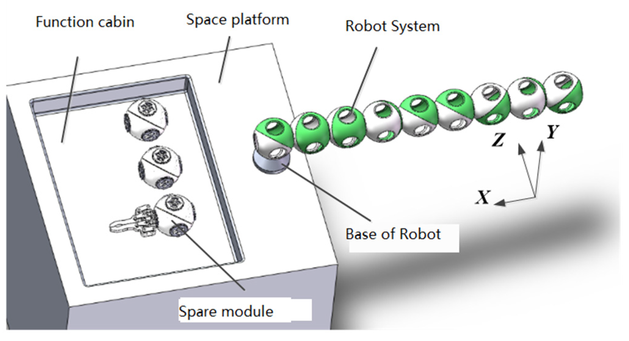
2.1. Space Mission Description

Reconfigurable robots can be used in fields such as on-orbit service and planet exploration, as they can change structures according to mission type or working environments. The existing space robots mainly adopt traditional configurations of joint linkage modes, which cannot achieve a self-reconstruction function. Thus, structural change is the basic function of space modular reconfigurable robots. Due to the modular docking and transformation solution, modular space robots can achieve system upgrades, maintenance, expansion, and other missions that are difficult to achieve with traditional space manipulators through the addition and removal of modules. To deal with this problem, this work firstly describes the space mission parameters for the addition of modules, as well as for removal and shape reconstruction, based on which the design principles of robot modules are determined.

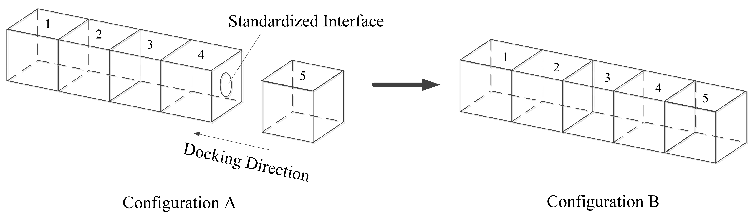
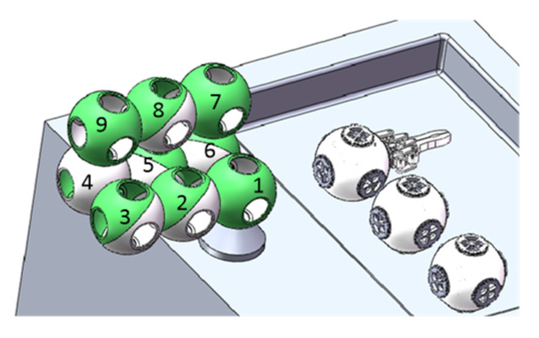
2.1.1. System Module Addition and Removal

As shown in Figure 1, each module is simplified and replaced by a cube. There are joint connections between each module or within the module itself, so that the relative changes in position and attitude between modules can be achieved. It is noted that every robot system is composed of four modules, i.e., it has at least four degrees of freedom. The robot can connect new modules through standardized docking surfaces to deal with many conditions such as lack of degrees of freedom, system upgrades, and end-load switching. The addition of module mission processes is as follows. The numbers on the diagram represent the names of the modules, same as Figure 2, Figure 3 and Figure 4.

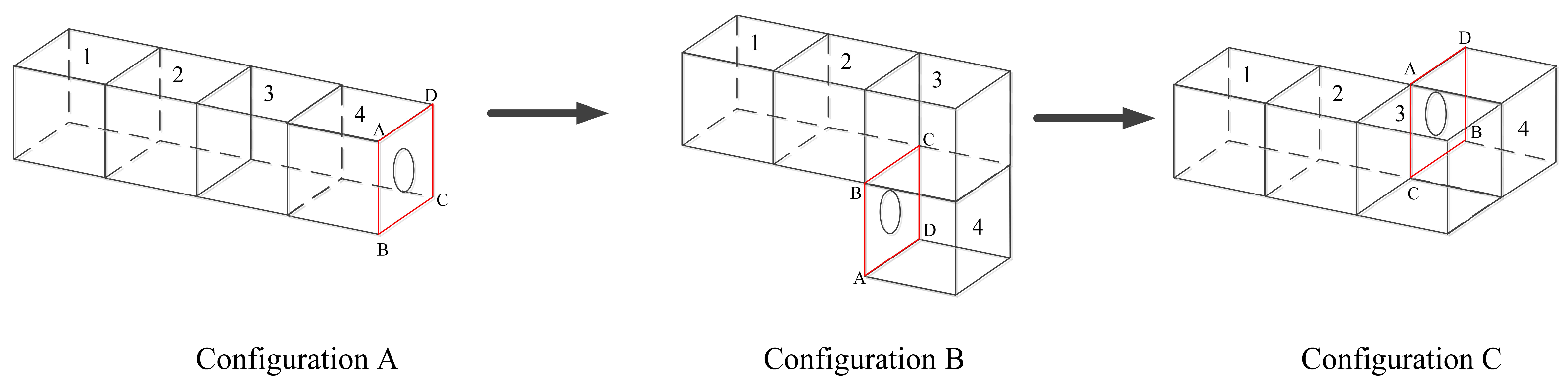
2.1.2. Position Changes between System Modules

When performing space missions, the modular space robot can realize structural transformations according to the different requirements of specific missions on the installation location, and transform the payload to the mission location to adapt to complex mission environments.
As shown in Figure 2, it is assumed that the robot system consists of multiple modules and each module is equipped with different mission loads, which can be used for different missions. For example, when module 4 is used as a working module, the working surface of module 4 is located outside the platform axis. Then, to achieve the requirement that the working surface of module 3 be exposed to the outside, modules 4 and 3 undergo a configuration transformation as a whole. Through allostery, the working interface of module 3 is exposed to the axial outside of the system and enters the working mode.
Through appropriate modular design and planned allosteric rules, the positions of modules can be interchanged and the functions of the entire reconfigurable system can be expanded.

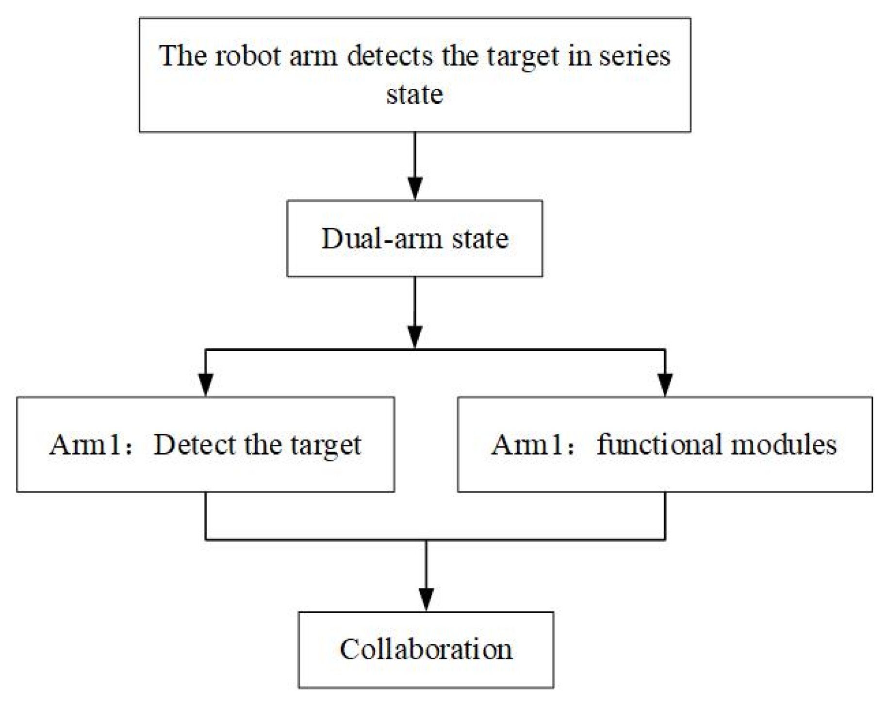
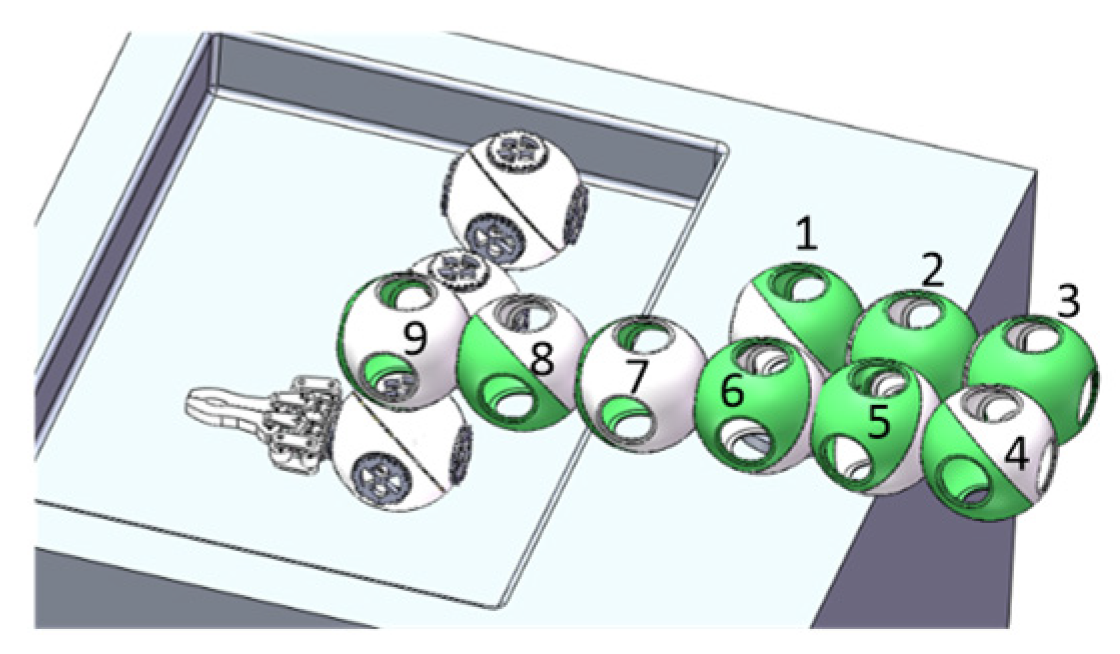
2.1.3. Reconstruction Changes from Single-Arm to Multi-Arm Robot System

During the actual mission, in order to achieve coordinated operation of the load, the robot can transform from a single-armed to double-armed or even multi-armed form. The mission process is shown in Figure 3.

2.1.4. Module Design Principles

Through the analysis of space missions and combined with the characteristics of reconstructed robots, the following design requirements are put forward, i.e.,
(1)
Versatility: the system is composed of unit modules and assembled into systems with different configurations and functions to meet different mission requirements.
(2)
Interface standardization: to meet the connection and disconnection between any two modules, the interface must adopt an isomorphic design and have a simple structure.
(3)
Self-driving capability: each module is the joint of a robot system, and the module contains a motor and a mechanical transmission system.
(4)
Independence: in order to achieve rapid reconstruction of the entire system, each module must have independent data processing capabilities, data transmission capabilities, and independent power supplies.
(5)
Platform: the robot module must have the ability to carry payloads, reserve a payload cabin inside the module, and set up a connecting mechanism outside the module.
(6)
Miniaturization: modular reconfigurable robots can use a certain number of modules to complete space missions in a limited space area and have the advantages of flexibility and adaptability.
The above design principles can ensure the fact that modular space robots can achieve flexible and changeable space missions, realize connection and disconnection between modules, as well as topological changes in the overall configuration, making the entire system highly adaptable to the environment.

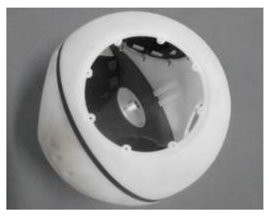
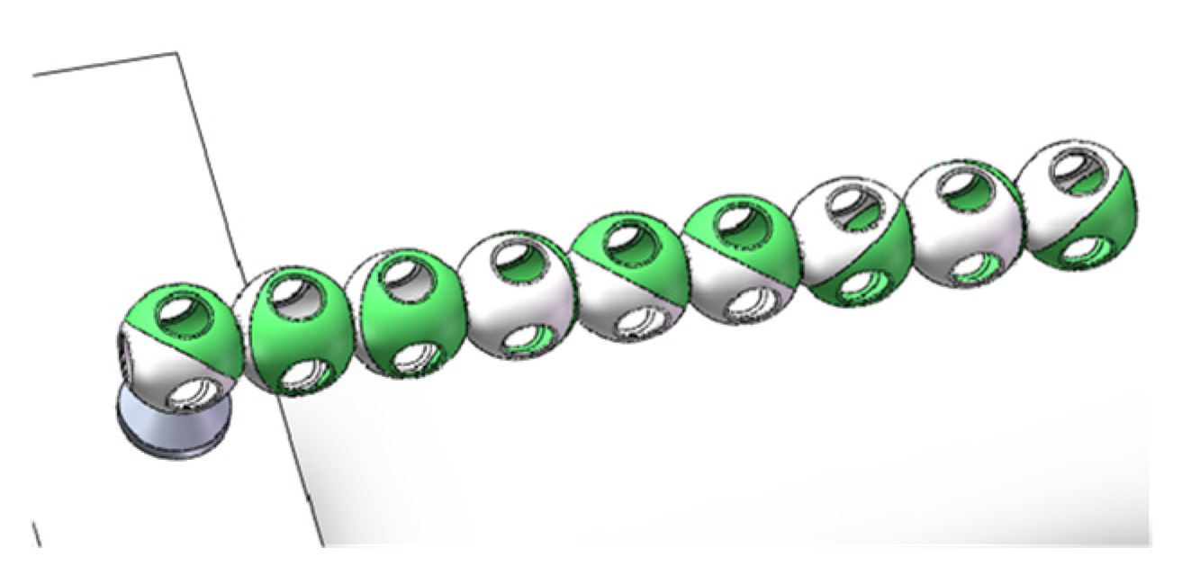
2.2. Unit Module Design

In order to better verify the expansion, shift, and reconstruction missions of the module, and to reduce the complexity of the system, the unit module only sets a single degree of freedom.
Modules are connected through universal docking surfaces to achieve system expansion. Meanwhile, in order to increase the connection reliability of the docking surfaces, the docking mechanism only completes the locking function without setting additional degrees of freedom of motion. Thus, the module motion joints can only be set inside the module and based on the built-in requirements of this joint, the entire module can be divided into two parts that can move with each other. Meanwhile, due to the complex space environment, the functional load and basic load of the module cannot be exposed outside of the module, which needs to set internal installation loads.
The unit module is composed of two relatively rotatable sub-modules. In order to ensure the scalability of the system, the two sub-modules are identical and have a symmetrical structure.
(1)
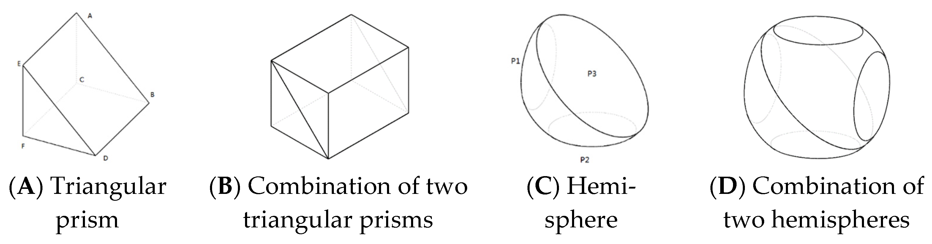
The two sub-modules have a common rotation surface that is connected and perpendicular to the rotation axis.
(2)
Modules can be connected through the connection surfaces opened on the sub-modules.
As shown in Figure 4, once the sub-module adopts a prism configuration, when the two sub-modules are rotated relative to each other, their rotation surfaces cannot overlap, and the external contour of the module will be destroyed. Once it is in a space environment, the internal load will also be exposed. Thus, in order to ensure that the module envelope shape remains uniform during the rotation of the sub-module, i.e., the outer contour of the rotation surface always coincides, it is appropriate to design the rotation surface as a circle.
During the rotation of the entire module, the outer contours of the two sub-cavities always coincide with each other, making the structure simpler and more compact. The module sub-cavity can be regarded as two symmetrical planes cut out of a hemisphere, and the attitude angle between the planes is 90°. When the structural sections in Figure 4C are increased to three, the three faces are made perpendicular to each other, and the following special geometry is obtained, called a quasi-tetrahedron. The resulting configuration becomes a configuration design based on the quasi-tetrahedron.

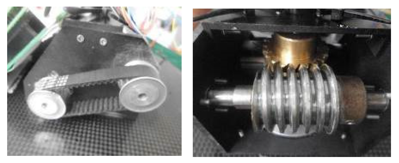
2.3. Unit Module Mechanism Design

This scheme adopts a quasi-tetrahedral configuration design. As can be seen in Figure 5, the sub-module is composed of two closed hemispherical shells. Each part is composed of a hemispherical shell and a supporting plate. The supporting plate is used to carry the transmission system, communication components, power supply system, etc. The hemispherical shell is designed based on a tetrahedral configuration, and the cross section can be equipped with a docking mechanism to connect other main joint modules or other non-joint modules.
It can be seen from Figure 6 that the hemispherical shell adopts an integrated design, and the hemispherical shell can support the plate so that it can be connected through the fixing hole. Each hemispherical shell has three mutually perpendicular annular surfaces, and the docking surface can be fixed through this annular surface.
Due to the complex shape of the hemispherical shell and the difficulty of metal cutting process, 3D printing rapid prototyping technology is used to process it. After processing and assembling the above parts, the assembly result of the main structure is shown in Figure 7.

2.3.1. Drive Selection and Transmission System Design
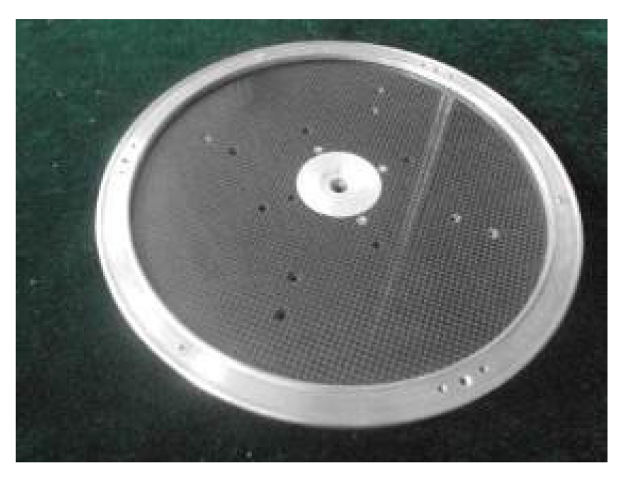
By mutual rotation between each module, one can realize the topological change of the overall system. For this purpose, corresponding drives and transmission mechanisms need to be designed. The conventional drive is generally a DC motor. When selecting the motor, try to make full use of the space inside the module and select a motor with appropriate torque and speed. Here, the FAULHABER2642CR motor (manufactured by the German von Haber Group, New York, NY, USA) is selected as the main motor of the module. Its properties are shown in Table 1.
The working process is as follows: install the worm gear, pulley, synchronous belt, motor, bearing, retaining ring, etc. on the designed support frame and then install the support frame on the active module support plate. The worm gear is connected to the torque output shaft and connected to the passive module through the flange. Connect and complete the assembly of the transmission system. The actual processed object and assembly result are shown in Figure 8.
In addition, as shown in Figure 9, a rotating guide rail is installed between modules. When rotation occurs between the two modules, the guide rail and the carbon fiber surface are used to rotate, which can greatly reduce the friction.

2.3.2. Power System

Inside the module, the module is monitored and controlled by connecting the communication module to the motor servo control system. The joint modular design requires that each module be an independent unit, so that the module is equipped with an independent power supply. Inside the module, the motor and its drive circuit board require a 24 V DC power supply, and the wireless module requires a 5 V DC power supply. Thus, a lithium battery and a voltage stabilizing module are provided to supply power to each device of the system. The wiring diagram of the entire system is shown in Figure 10.
In order to make full use of the internal space of the module, each subsystem is installed in two sub-cavities. The main motor and transmission system are installed in the active sub-module of the system, that is, the wireless module and power supply are installed in the passive sub-module. In order to solve the problem of wire winding during rotation, the transmission shaft is designed as a hollow shaft, and the wiring is arranged inside the shaft. The corresponding wires on the stator of the conductive slip ring are connected to the active module motor and motor control board to achieve alignment. Conductive slip ring and DC step-down module as shown in Figure 11 below.

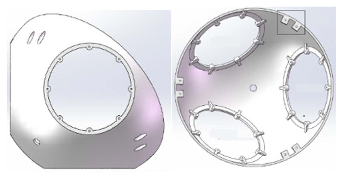
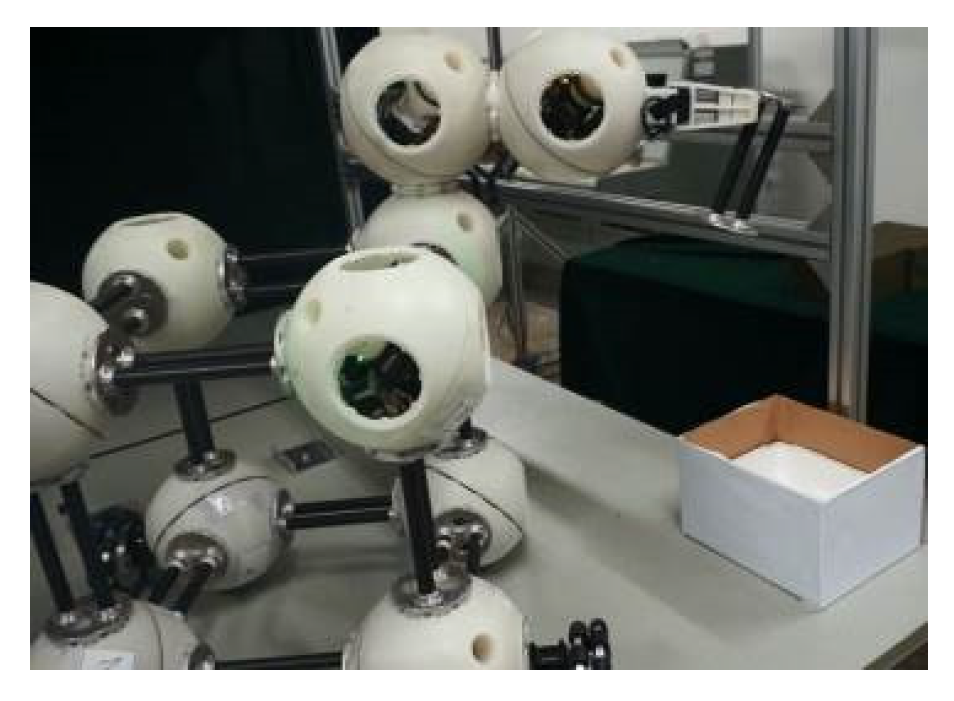
2.3.3. System Assembly

In this section, the designed parts are processed and assembled, and the power supply, motor, transmission mechanism, voltage reduction module, communication equipment, etc. are fixed and installed inside the structure in turn. The rotation of the motor is controlled to realize the mutual rotation of the active sub-module and the passive sub-module and experimentally verified to ensure that there is no limit to the attitude angle. The overall configuration is shown in Figure 12.

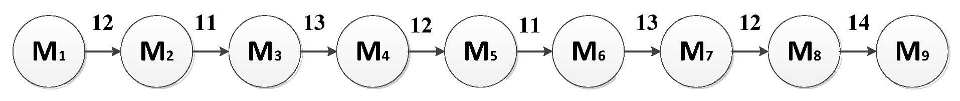
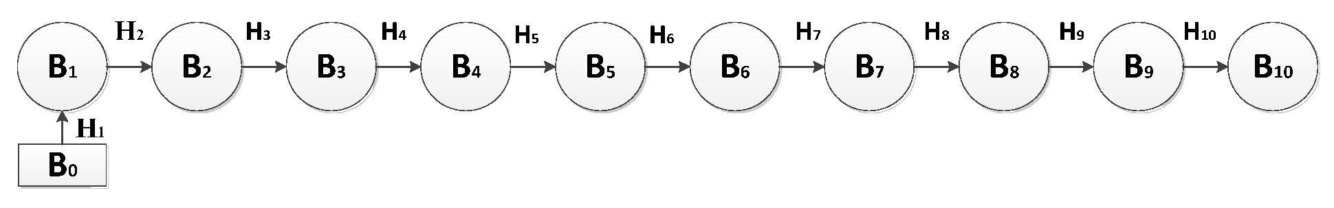
3. Dynamic Modeling of Spatial Modular Robot Based on R-W Method

3.1. Joint Motion Model

The joint in the multi-body system is an abstraction of the constraints of adjacent rigid bodies. The relative motion of the joint can be described by the relative motion relationship of the reference system fixed on the two parts.
The joint in the multi-body system is an abstraction of the constraints of the adjacent rigid bodies. The relative motion of the joint can be described by the relative motion relationship of the reference system fixed on the two parts. One of the two parts serves as a reference for relative motion, and the conjoined base on the part becomes the local base of the joint, which is recorded as e ¯ h 0 . Its base point is recorded as Q and the conjoined base of another component that moves relative to the base is called the moving base of the joint, denoted as e _ h . Its base point is recorded as P and vector diameter is denoted as h , which describes the relative motion of the joint. The derivative of the vector h in local basis e _ h 0 with respect to time is v r . The relative acceleration is v r and the direction cosine matrix of the dynamic basis relative to the bulk basis is recorded as A _ h , which describes the posture of the dynamic base relative to the noumenal base. The relative angular velocity vector of the dynamic base relative to the body base is ω r . The coordinate matrix of any vector such as a in basis e _ h 0 is called the local coordinate matrix or joint coordinate matrix of the joint, denoted as a . The coordinate system is shown in Figure 13.
For the space robot module developed in this work, its joint type is a rotating joint, which is a joint with only one relative rotational degree of freedom. Local basis e _ h 0 and dynamic basis e _ h are established, respectively, at the midpoint of the rotation axis in which P coincides with Q . The basis vector e _ h 0 = e _ h = p 1 , p 1 is the unit vector of the joint axis and the rotation angle q 1 is the generalized coordinate of the rotation joint. Assume that the initial rotation angle q 10 = 0 , then one has
A _ h = 1 0 0 0 C 1 S 1 0 S 1 C 1
where S 1 = sin q 1 , C 1 = cos q 1 .
The relative angular velocity vector of the rotating joint is ω r = p 1 q ˙ 1 . Since the vector p 1 is fixed to the joint foundation, the relative angular acceleration ω r is ω r = p 1 q ˙ 1 . The local coordinate matrix of the unit vector is p 1 = ( 1 0 0 ) T , and the coordinate matrix of relative velocity and relative angular acceleration vector is ω r = p 1 q ˙ 1 , ω r = p 1 q ¨ 1 . Since the two base points Q and P always coincide, the relative displacement, relative velocity, and relative acceleration of the base point are all zero.
The base in a free-floating state and 6 degrees of freedom is regarded as the case that is connected to the inertial reference frame through 6 degrees of freedom virtual joint.
The generalized coordinate of relative motion of joints is q _ = ( q _ t T q _ r T ) T and the vector diameter h and generalized expressions of velocity, acceleration, angular velocity, and angular acceleration are h = H _ h T q _ , v r = H _ h T q _ ¨ , ω r = H _ Ω T q _ ¨ + η , respectively.

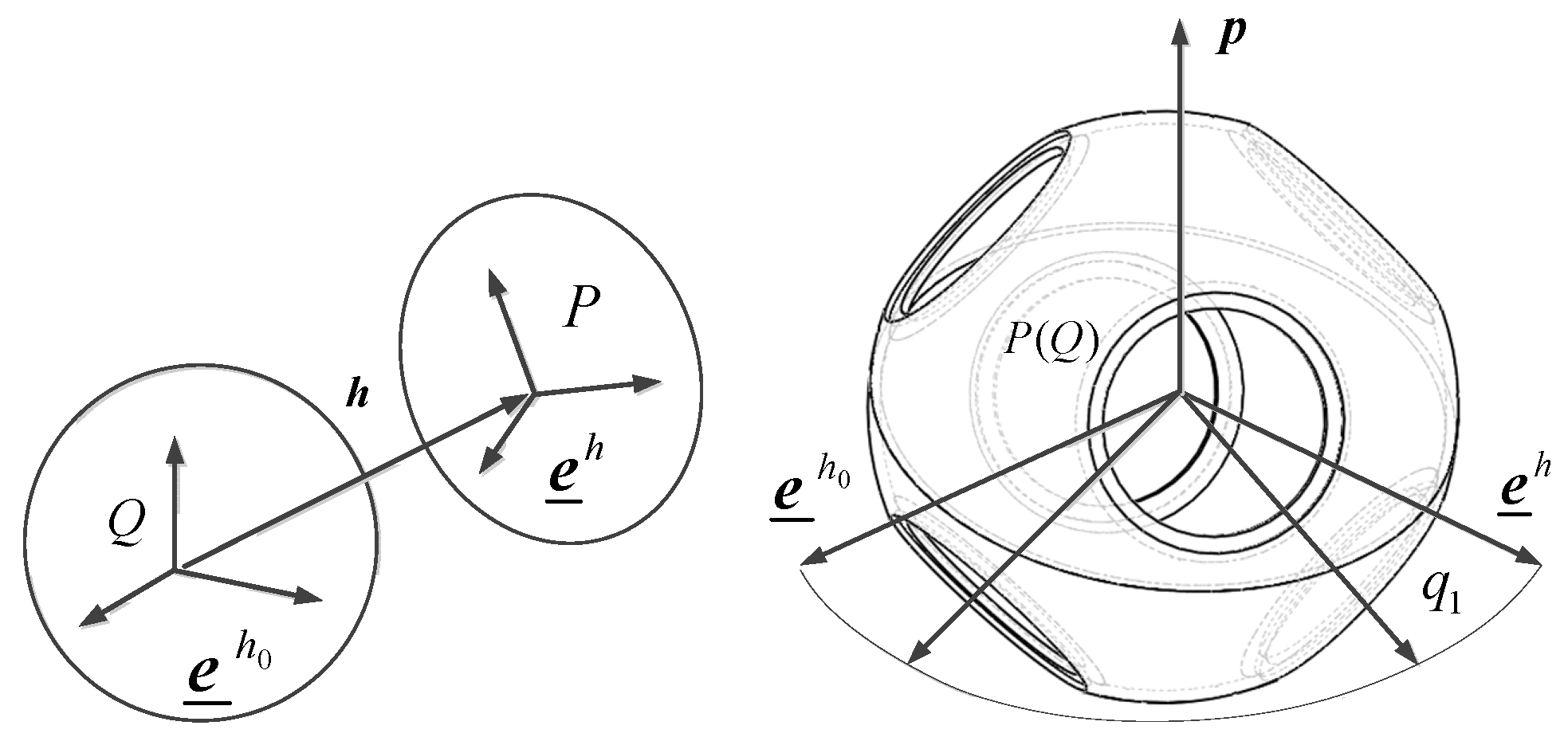
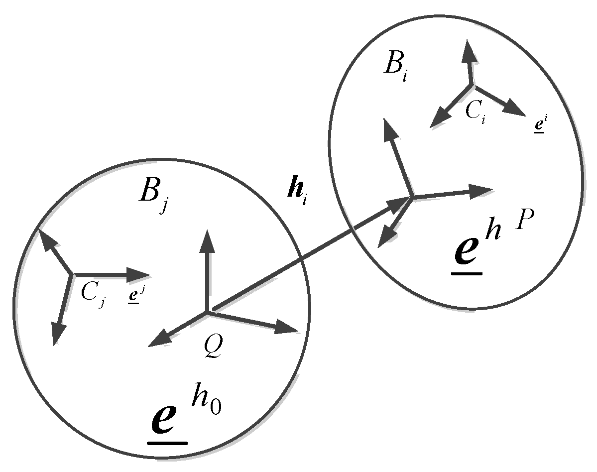
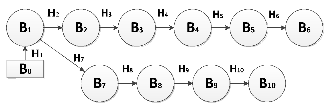
3.2. Attitude Motion of Each Rigid Body in the System

For a tree system composed of N rigid bodies, the adjacent rigid body associated with joint Hi ( i = 1 , , N ) is denoted as B j and B i ( B j is internal rigid body of B i ) whose conjoined base are e _ j and e _ i , respectively. Dynamic base e _ h of Hi is fixed to point P of the rigid body B i . The generalized coordinate matrix of this joint is recorded as q _ i . In local basis e _ h 0 , the constant directional matrices of e _ j and e _ h are written as Q _ j and P _ j . The direction cosine matrix of the dynamic base e _ h of joint Hi with respect to the reference base e _ h 0 is recorded as A _ i h . The direction cosine matrix of the rigid body B i relative to B j is A _ j i = Q _ j A _ i h P _ j . Relative kinematics relationship between adjacent rigid bodies in tree systems is shown in Figure 14.
The relative attitude of the adjacent rigid body depends on the joint’s orientation matrix, which is a function of the joint’s generalized coordinates. If the degrees of freedom of each joint of the system are δ i , the motion of the system will be described by the generalized coordinate matrix of the system composed of the generalized coordinates of each joint.
The attitude of a rigid body B i ( i = 1 , , N ) with respect to the overall base of the system can be described by its cosine matrix with respect to the overall base direction of the system. Due to the properties of the directional cosine matrix, with the help of the inscribed rigid body array L ( i ) , the rigid body has the following recursive formula for the directional cosine matrix A _ i :
A _ i = A _ 0 A _ 01 i = 1 A _ L ( i ) A _ L ( i ) i i = 2 , N
where A _ 0 is the cosine matrix of the root object with respect to the overall base direction of the system. The direction cosine matrix of the local basis of joint H i is recorded as A _ i h 0 and the direction cosine matrix is a function of the generalized coordinates of all joints on the road, i.e., A _ i h 0 = A _ L ( i ) Q _ L ( i ) .
The absolute angular velocity of the rigid body B i ( i = 1 , , N ) is recorded as ω i . Based on the angular velocity superposition principle, the absolute angular velocity of the rigid body B i can be expressed as the following vector recursion formula.
ω r = ω r + ω 0 i = 1 ω r i + ω l ( i ) i = 2 , N
where ω 0 is the absolute angular velocity of the root object. From another perspective, the absolute angular velocity of B i is the vector sum of the relative angular velocities and ω 0 of all rigid bodies on path B i to B 0 . According to the definition of the path matrix, considering that the path matrix element corresponding to the joint H k not on path B i to B 0 is zero, the absolute angular velocity of the rigid body B i can also be expressed as:
ω i = B k ( B i ) ω r k + ω 0 = k = 1 N T k i ω r k + ω 0 ( i = 1 , , N )
The negative sign in the formula is because for regular labels, the elements of the path matrix are negative. The absolute angular velocity vectors of these N rigid bodies can be combined into a vector matrix formula as follows:
ω _ = T _ T ω r + ω 0 1 _ N
ω _ r = H _ i Ω T q _ ˙
The relationship between the absolute angular velocity vector of each rigid body in the system and the generalized coordinate derivative is as follows:
ω _ = β _ q ˙ _ ω r + ω 0 1 _ N
The angular velocity of the above equation is changed to:
Δ ω _ = β _ Δ q ˙ _
In the equation β _ = ( H _ Ω T _ ) , H _ Ω is an N-order diagonal block vector matrix H _ j Ω T , with the vector matrix as an element, and β _ is an N × N order vector block matrix in which the vector block array in the i-th row and j-th column is T j i H _ j Ω T . The transpose of its channel matrix T _ and vector block matrix β _ are as follows.
T ¯ = 1 0 0 0 0 0 1 1 0 0 0 0 1 0 1 0 0 0 1 0 1 1 0 0 1 0 0 0 1 0 1 0 0 0 0 1   β _ = H _ 1 Ω T 0 0 0 0 0 H _ 1 Ω T H _ 2 Ω T 0 0 0 0 H _ 1 Ω T 0 H _ 3 Ω T 0 0 0 H _ 1 Ω T 0 H _ 3 Ω T H _ 4 Ω T 0 0 H _ 1 Ω T 0 0 0 H _ 5 Ω T 0 H _ 1 Ω T 0 0 0 0 H _ 6 Ω T
It is not difficult to see that the vector block β _ is a lower triangular vector block matrix, which is consistent with the position of the transposed non-zero term of the channel matrix T _ . As long as the non-zero item in the j-th column is replaced by H _ j Ω T , β _ will be generated.
The first derivative of the angular velocity on the global coordinate base is
ω ˙ i = k = 1 N T k i ω ˙ r k + ω 0 ( i = 1 , , N )
Considering ω ˙ r i = ω r i + ω L ( i ) × ω r i , we can get the vector matrix formula composed of the N rigid body absolute angular acceleration vector, i.e.,
ω ˙ = T _ T ω _ r + ω ˙ 0 1 _ N T _ T ζ _
where ζ i = ω ˙ L ( i ) × ω r i .
Considering ω r = H _ Ω T q ¨ _ + η _ , the above equation can be rewritten as the final expression of angular acceleration:
ω ˙ _ = β _ q ¨ _ + ω ˙ 0 1 _ N T _ T ( ζ _ + η _ )

3.3. Position Motion of Each Rigid Body in the System

For a multi-rigid body system connected by rotating joints such as rotary joints and universal joints, it will become a multi-rigid body system with rotating joints. Its characteristic is that the joint points on the adjacent objects of all joints coincide, and there is only relative rotation without position motion. The robot system developed in this work is exactly such a system. The position, angular velocity, and acceleration analysis of each rigid body’s center of mass in the system will designate the distribution of the joint points on the rigid body. Thus, in describing the basic parameters of a multi-rigid body system, in addition to the topological configuration parameters of the system, it is also necessary to give the distribution of the joints on each object. Thus, before discussing the position, velocity, and acceleration of the center of mass of each rigid body in the system, we will first introduce the body joint vector and pathway vectors.
For a multi-rigid body system composed of N objects, the center of mass of the rigid body B i ( i = 1 , , N ) is recorded as C i . The vector pointing from C i to a joint point on the rigid body is defined as the body joint vector of the joint H j , which is recorded as c i j , where i represents the fixed rigid body and j represents the joint pointed by this vector.
If the joint H j is not related to B i , c i j = 0 for a root object whose motion is known, the starting point C 0 of the body joint vector is generally taken at the joint H 1 . Since each joint involves two body joint vectors, the non-zero body joint vector for the tree system is 2N − 1. Their coordinate matrix in the conjoined bases is one of the basic parameters describing the system.
For a tree system, using the correlation matrix elements, the weighted body joint vectors are
C i j = S i j c i j ( i = 1 , , N ; j = 1 , , N )
There are still 2N − 1 non-zero weighted body joint vectors. S i j negates c i j , pointing to the inscribed joint and C i j is in the same direction as the joint H j , deviating from the direction of B 0 . The weighted joint vector C i j is used to form an N-order vector square matrix to become the body joint vector matrix C _ . This vector matrix describes the distribution of joints of each object. The body joint vector matrix of the robot system is
C _ = c 11 c 12 c 13 0 c 15 c 16 0 c 22 0 0 0 0 0 0 c 33 c 34 0 0 0 0 0 c 44 0 0 0 0 0 0 c 55 0 0 0 0 0 0 c 66
Each object has only one internal joint in the tree systems and the internal joint of the rigid body B i is H i . The connected vector d i k from H i in B i can be defined as a pathway vector. When k i , this vector points to another joint on B i , which is located on the path from B i to B k . When k = i , this vector points to the center of mass of the object.
The N-order vector square matrix d _ containing d i k is called the path vector matrix, which describes the joint distribution of each object. The path vector matrix d _ of the tree system is
d _ = d 11 d 12 d 13 d 14 d 15 d 16 0 d 22 0 0 0 0 0 0 d 33 d 34 0 0 0 0 0 d 44 0 0 0 0 0 0 d 55 0 0 0 0 0 0 d 66 = d 11 d 12 d 13 d 13 d 15 d 16 0 d 22 0 0 0 0 0 0 d 33 d 34 0 0 0 0 0 d 44 0 0 0 0 0 0 d 55 0 0 0 0 0 0 d 66
Both the body joint vector and the path vector describe the position of the joint point on the rigid body, but the starting point of the vector is different and their mathematical relationship can be described as d _ = C _ T _ .
The vector radius of the base point of the conjoined base with respect to the base point of the overall base of the system is
r i = k : B k ( B i ) d r k + r 0
where, k is the subscript of all rigid bodies B k on the path from B i to B 0 . The coordinate matrix of the above formula in the overall basis e _ is
r _ i = k : B k ( B i ) d _ r k + r _ 0 = k : B k ( B i ) A _ k d _ r k + r _ 0
The equation only contains the direction cosine matrix A _ k of all rigid bodies on the path from the rigid body B i to B 0 and constant coordinate matrix of the path matrix in the conjoined basis. Thus, the centroid coordinate matrix of B i is a function of the generalized coordinates of all rigid internal joints on the path from B i to B 0 . Thus, the above equation can be written as
r _ = d _ T 1 _ N + r 0 1 _ N
The velocity of the centroid can be calculated through differentiation, i.e.,
r ˙ i = k : B k ( B i ) d ˙ r k + r ˙ 0 ( i = 1 , , N )
Since the vector is fixed to the rigid body B k , substituting d ˙ k i = ω k × d k i into the above equation yields
r _ ˙ = d _ T × ω + r ˙ 0 1 _ N
The relationship between the velocity of the base point of a rigid body B i and the derivative of the generalized coordinates can be recorded as
r _ ˙ = α _ q ˙ _ + v _
The angular velocity of the above equation is changed to:
Δ r _ ˙ = α _ Δ q ˙ _
where
α _ = - ( H _ Ω T × d _ ) T
v _ = r ˙ 0 1 _ N d _ T × ω 0 1 _ N
α _ = H _ 1 Ω T × d 11 0 0 0 0 0 H _ 1 Ω T × ( d 12 + d 22 ) H _ 2 Ω T × d 22 0 0 0 0 H _ 1 Ω T × ( d 13 + d 33 ) 0 H _ 3 Ω T × d 33 0 0 0 H _ 1 Ω T × ( d 14 + d 34 + d 44 ) 0 H _ 3 Ω T × ( d 34 + d 44 ) H _ 4 Ω T × d 44 0 0 H _ 1 Ω T × ( d 15 + d 55 ) 0 0 0 H _ 5 Ω T × d 55 0 H _ 1 Ω T × ( d 16 + d 66 ) 0 0 0 0 H _ 6 Ω T × d 66
The acceleration of the center of mass can be found by taking two derivatives with respect to time:
r ¨ i = k : B k ( B i ) d ¨ r k + r ¨ 0 ( i = 1 , , N )
Since the vector is fixed to the rigid body B k , substituting d ¨ k i = ω ˙ k × d k i + ω k ( ω k × d k i ) into the above equation yields
r ¨ i = k : B k ( B i ) d k i   ×   ω ˙ k + k : B k ( B i ) ω k ( ω k × d k i ) + r ¨ 0
i.e.,
r _ ¨ = α _ q ¨ + w _
where
w i = r ¨ 0 + k : B k ( B i ) [ ω k × ( ω k × d k i ) + σ k × d k i ]

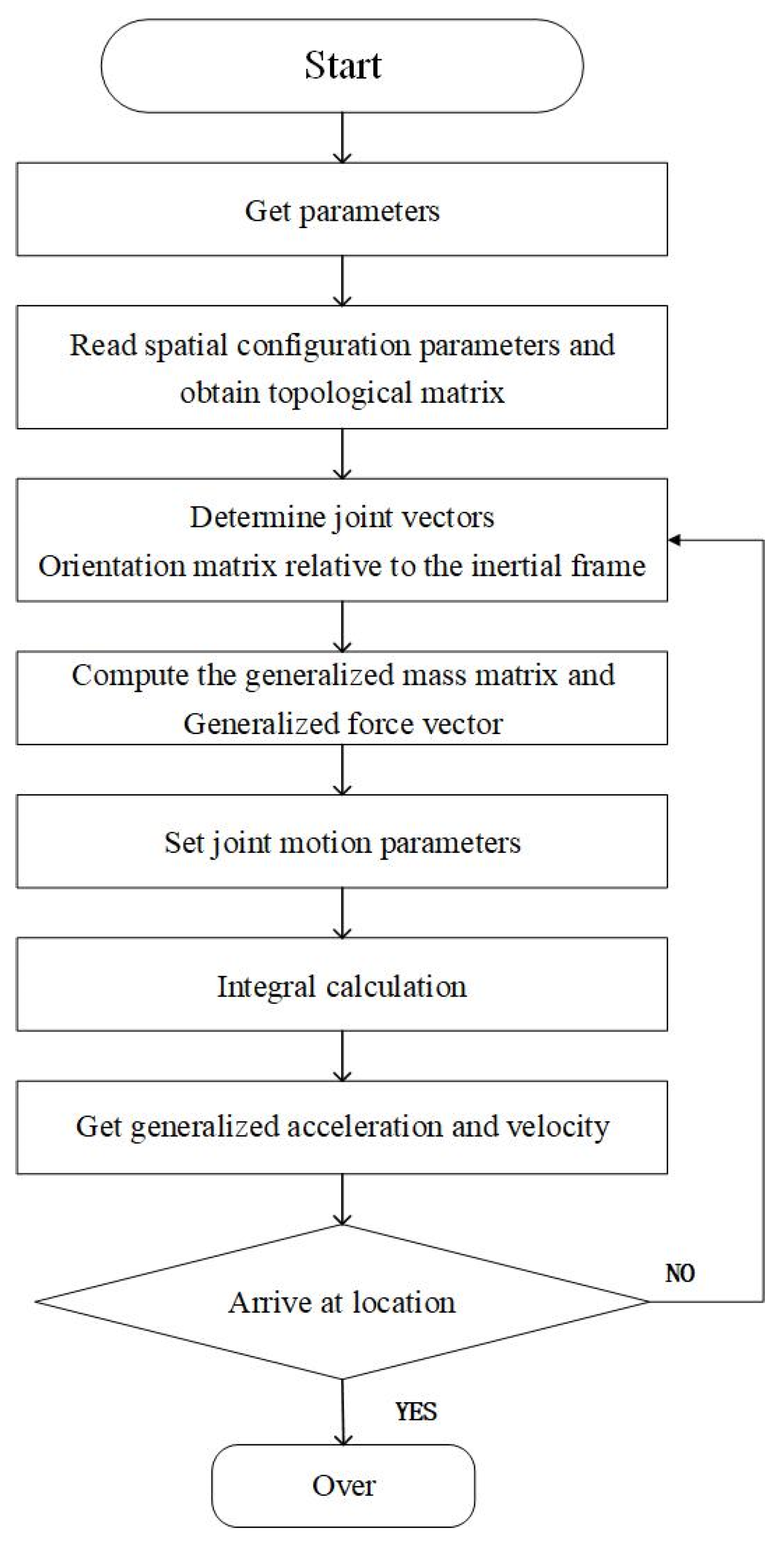
3.4. Establishment of Kinetic Equations

In the tree system composed of N rigid bodies, the mass of rigid body B i is m i and the moment of inertia is J i . The principal vector of the external force on the rigid body and the principal moment relative to the center of mass are F i o and M i o , respectively. According to the velocity variation principle, the variational form of the dynamic equation of the system is
i = 1 N [ Δ r ˙ ( - m i r ¨ i + F i o ) + Δ ω i ( J i ω ˙ i ε i + M i o ) ] + Δ P = 0
where Δ P represents the virtual power exerted by the internal forces between objects in the system.
The relationship between the generalized force matrix F _ q of the system’s generalized coordinates and Δ P is:
Δ P = Δ q _ ˙ T F _ q
where ε i = ω i × ( J i ω i ) , and the matrix form is
Δ r ˙ _ T ( - m _ r ¨ _ + F _ o ) + Δ ω _ T ( J _ ω ˙ _ ε _ + M _ o ) + Δ P = 0
The differential equation of the dynamic system can be integrated into:
Z _ q _ ¨ = z _
where
Z = α _ T m _ α _ + β _ T J _ β _ , z = α _ T ( F _ 0 m _ w _ ) + β _ T ( M _ J _ σ _ ε _ ) + F _ q .
It should be mentioned that the inertial parameters of each object and the path vector matrix in this differential equation will be inputted into the calculation module to perform dynamic simulation analysis on specific space missions.

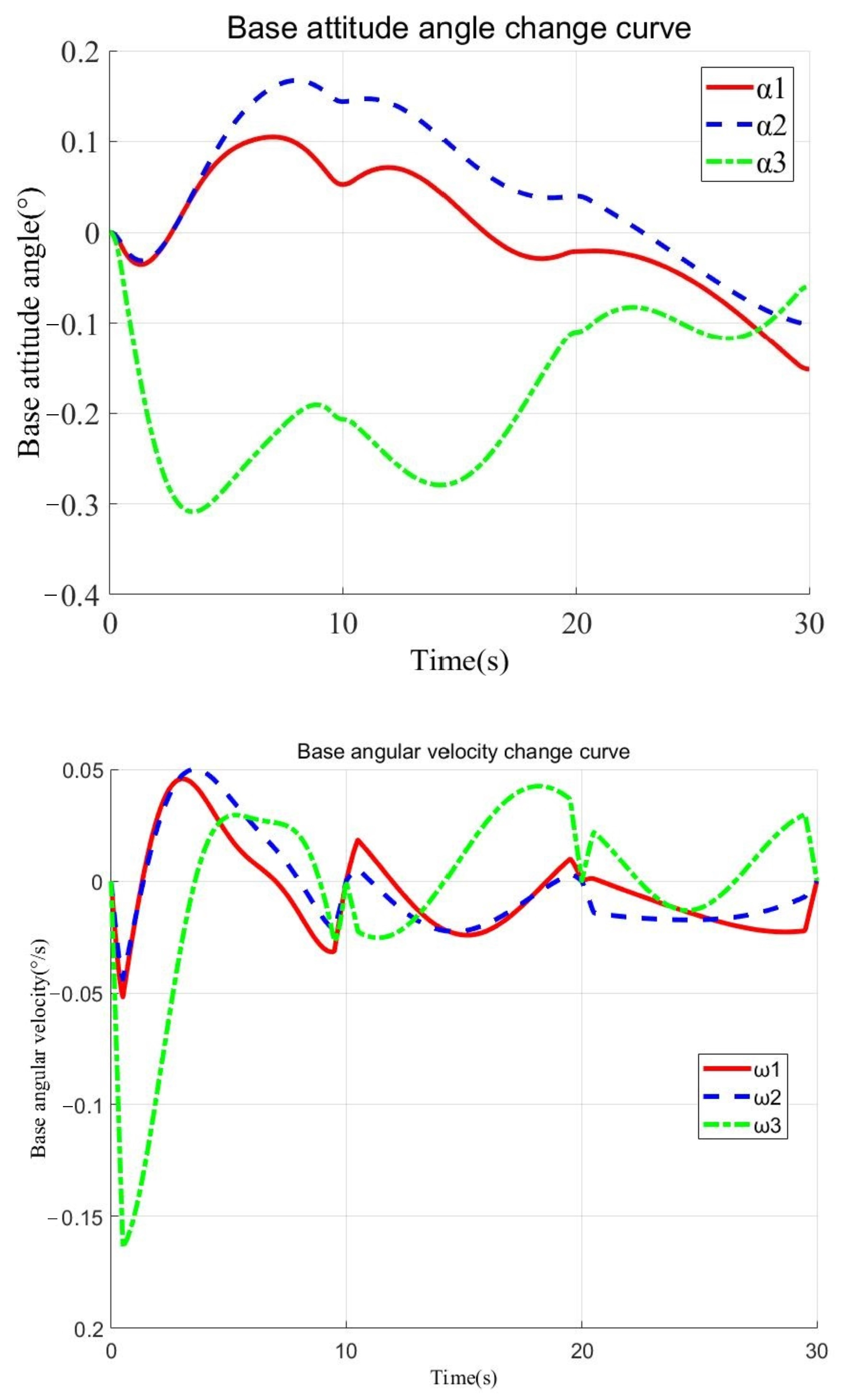
4. Dynamic Model Simulation Analysis

In order to verify the developed system topology and dynamic modeling method, the following mission scenario is designed. The robot system is mounted on the space platform to perform maintenance function on faulty targets. Each module of the robot is equipped with an observation load, flaw detection load, communication load, and basic load. The space platform has a functional cabin that carries capture modules, maintenance modules, spare modules, etc. First, the robot system realizes the detection and scanning of long-distance targets through tandem mode. Then, the robot system changes to the multi-arm mode, where one of the robot arms is connected to the required functional module from the platform function cabin and the other robotic arm continues to detect the target location. That is to say, the two robotic arms collaborate with each other to perform corresponding operation missions on the target. All simulations were conducted under low gravity conditions. The mission flow chart is shown in Figure 15.
The initial state of the system is as shown in Figure 16. Each module consists of a green hemisphere and a white hemisphere.
The topology of the robot system in the initial state is described in Figure 17.
According to the described connection relationship between modules, one first determines the rotation axis vector of M1 and then obtains the orientation vectors of all modules.
Transformed into a multi-body system problem description, the system topology is shown in Figure 18, where B1 is the object composed of module one and the platform, B2-B9 are new objects formed by connecting adjacent modules, and B10 is the passive sub-module of module 9. H1 is the virtual hinge from B1 to the inertial coordinate system, H2-H10 are all rotation hinges of the module, and its constraint vector is the projection of the rotation axis vector in the inertial system. Thus, according to the topological configuration, the system topology description matrix is obtained.
The correlation matrix and pathway matrix are:
    H 1         H 2         H 3         H 4         H 5         H 6         H 7         H 8         H 9         H 10 S ¯ = B 1 B 2 B 3 B 4 B 5 B 6 B 7 B 8 B 9 B 10 1 1 1 1 1 1 1 1 1 1 1 1 1 1 1 1 1 1 1 B 1         B 2         B 3         B 4         B 5         B 6         B 7         B 8         B 9         B 10 T ¯ = H 1 H 2 H 3 H 4 H 5 H 6 H 7 H 8 H 9 H 10 1 1 1 1 1 1 1 1 1 1 1 1 1 1 1 1 1 1 1 1 1 1 1 1 1 1 1 1 1 1 1 1 1 1 1 1 1 1 1 1 1 1 1 1 1 1 1 1 1 1 1 1 1 1 1
The array of internal objects is L ¯ = 0 1 2 3 4 5 6 7 8 9 .
The mass of the platform base is set to be 800 kg. According to the mission design, the robot system reconfiguration process is as shown in the following three stages.
Reconfiguration stage 1: movement of modules No. 3, No. 4, No. 6, and No. 7. The initial configuration of the modules is shown in Figure 19.
Rotation angles of modules No. 3, No. 4, No. 6, and No. 7 will be changed to be 240°, 120°, −120°, and 120°, respectively. The symbol indicates the direction of rotation.
The configuration in Figure 20 is obtained.
Reconfiguration stage 2: Module 6 is disconnected from module 5 and module 6 establishes a connection relationship with module 1. The robot system changes from a single-arm system to a dual-arm system. After that, control the movement of module No. 6 and module No. 7, and the rotation angles are 120° and −120°, respectively. The configuration in Figure 21 is obtained.
The system topology is shown in Figure 22.
The system topology matrix can be described as
    H 1         H 2         H 3         H 4         H 5         H 6         H 7         H 8         H 9         H 10 S ¯ = B 1 B 2 B 3 B 4 B 5 B 6 B 7 B 8 B 9 B 10 1 1 1 1 1 1 1 1 1 1 1 1 0 1 1 1 1 1 1 1 B 1         B 2         B 3         B 4         B 5         B 6         B 7         B 8         B 9         B 10 T ¯ = H 1 H 2 H 3 H 4 H 5 H 6 H 7 H 8 H 9 H 10 1 1 1 1 1 1 1 1 1 1 1 1 1 1 1 0 0 0 0 1 1 1 1 0 0 0 0 1 1 1 0 0 0 0 1 1 0 0 0 0 1 0 0 0 0 1 1 1 1 1 1 1 1 1 1
The array of internal objects is L ¯ = 0 1 2 3 4 5 1 7 8 9 .
The masses of B1 and B6 have changed and need to be reacquired during the kinetic analysis.
Reconfiguration stage 3: Module 9 is connected to the capture module in the functional cabin, and the capture module is defined as module 10, thereby forming a new robot system with capture function. At this time, the topology of the robot system also changes, adding a module and a rotating hinge, which will not be elaborated here. After the docking process, the motions of modules 6, 10, 3, and 4 are controlled. The rotation angles are -120°, 120°, 120°, −240°, −120°, respectively, and one can get the final robot configuration shown in Figure 23.
The program flow chart is shown in Figure 24.
In the simulation, the time of each stage is set to 10 s and the rotating joint performs uniform acceleration and deceleration motions at the beginning and end of each stage for 0.5 s. Through simulation analysis, the time response of the base and the control torque of each hinge can be obtained. Figure 25 shows the time response of the base attitude angle and angular velocity, from which one can see that the attitude angle is no more than 0.32° and the angular velocity converges to a region within 0.05°/s. Similarly, Figure 26 gives the time response of center for mass position and velocity and Figure 27 gives the time response of control torque of all module joints. By adding motion constraints, this simulation demonstrates the motion of a modular space robot during on-orbit operation, verifies the flexibility and feasibility of the dynamic modeling method, and provides information for the control and application of the modular space robot system.

5. Conclusions

This paper proposes a novel space robot configuration and working mode, and the module design implementation and dynamic modeling are analyzed. In detail, the reconfigurable space robot mission and configuration design, reconfigurable space robot module, system design optimization and prototype implementation, and system experimental testing are performed and analyzed. Based on the analysis of the robot space mission, a configuration design scheme for a modular reconfigurable space robot is developed. The corresponding dynamic model reconstruction has also been validated through specific space tasks. This modular robot has a rich number of structural forms and corresponding real-time generated dynamic models, which have more obvious advantages compared to traditional space robots. It should be mentioned that the complexity of dynamic models requires a high computational power for computers, which poses a huge challenge based on existing space computer technology. In addition, the numerous modules may pose certain challenges to the fault tolerance performance of the system. The aforementioned challenges will be the future research direction to be overcome.

Author Contributions

Conceptualization, X.Y.; funding acquisition: X.Y.; writing, D.Y.; methodology, D.Y.; software, D.Y.; validation, D.Y.; investigation, M.G. All authors have read and agreed to the published version of the manuscript.

Funding

This work was supported by the National Natural Science Foundation of China (U2013206, 11972026).

Institutional Review Board Statement

No applicable.

Informed Consent Statement

Not applicable.

Data Availability Statement

The data presented in this study are available in the article.

Conflicts of Interest

The authors declare no conflict of interest.

References

  1. Schmitz, D.; Khosla, P.; Kanade, T. The CMU reconfigurable modular manipulator system. In Proceedings of the International Symposium and Exposition on Robots, Sydney, Australia, 6–10 November 1988; pp. 473–488. [Google Scholar]
  2. Zhang, Y.; Oğuz, S.; Wang, S.; Garone, E.; Wang, X.; Dorigo, M.; Heinrich, M.K. Self-reconfigurable hierarchical frameworks for formation control of robot swarms. IEEE Trans. Cybern. 2023, 1–14. [Google Scholar] [CrossRef] [PubMed]
  3. Yim, M.; Shen, W.-M.; Salemi, B.; Rus, D.; Moll, M.; Lipson, H.; Klavins, E.; Chirikjian, G.S. Modular Self-Reconfigurable Robot Systems: Grand Challenges of Robotics. IEEE Robot. Autom. Mag. 2007, 14, 43–52. [Google Scholar] [CrossRef]
  4. Yim, M.; Duff, D.G.; Roufas, K.D. Polybot: A modular reconfigurable robot. In Proceedings of the 2000 ICRA. Millennium Conference. IEEE International Conference on Robotics and Automation Symposia Proceedings (Cat. No.00CH37065), San Francisco, CA, USA, 24–28 April 2000; pp. 514–520. [Google Scholar]
  5. Castano, A.; Shen, W.M.; Will, P. CONRO: Towards deployable robots with inter-robots metamorphic capabilities. Auton. Robot. 2000, 8, 309–324. [Google Scholar] [CrossRef]
  6. Moeckel, R.; Jaquier, C.; Drapel, K.; Dittrich, E.; Upegui, A.; Ijspeert, A. YaMoR and bluemove—An autonomous modular robot with bluetooth interface for exploring adaptive locomotion. In Proceedings of the 8th International Conference on Climbing and Walking Robot, London, UK, 30 June 2005; pp. 685–692. [Google Scholar]
  7. Mondada, F.; Guignard, A.; Bonani, M.; Bar, D.; Lauria, M.; Floreano, D. SWARM-BOT: From concept to implementation. In Proceedings of the IEEE/RSJ International Conference on Intelligent Robots and Systems (IROS 2003) (Cat. No.03CH37453), Las Vegas, NV, USA, 27–31 October 2003; pp. 1626–1631. [Google Scholar]
  8. Wei, H.; Liu, M.; Li, D.; Wang, T. A novel self-assembly modular swarm robot-docking mechanism design and self-assembly control. Jiqiren (Robot) 2010, 32, 614–621. [Google Scholar]
  9. Zykov, V.; Mytilinaios, E.; Desnoyer, M.; Lipson, H. Evolved and Designed Self-Reproducing Modular Robotics. IEEE Trans. Robot. 2007, 23, 308–319. [Google Scholar] [CrossRef]
  10. Zykov, V.; Chan, A.; Lipson, H. Molecubes: An Open-Source Modular Robotics Kit. In Proceedings of the IROS, San Diego, CA, USA, 29 October–2 November 2007. [Google Scholar]
  11. Bonardi, S.; Blatter, J.; Fink, J.; Moeckel, R.; Jermann, P.; Dillenbourg, P.; Jan Ijspeert, A. Design and Evaluation of a Graphical iPad Application for Arranging Adaptive Furniture; Institute of Electrical and Electronics Engineers Inc.: Paris, France, 2012. [Google Scholar]
  12. Sprowitz, A.; Pouya, S.; Bonardi, S.; Van Den Kieboom, J.; Möckel, R.; Billard, A.; Dillenbourg, P.; Jan Ijspeert, A. Roombots: Reconfigurable Robots for Adaptive Furniture. IEEE Comput. Intell. Mag. 2010, 5, 20–32. [Google Scholar] [CrossRef]
  13. Murata, S.; Yoshida, E.; Kamimura, A.; Kurokawa, H.; Tomita, K.; Kokaji, S. M-TRAN: Self-Reconfigurable Modular Robotics System. IEEE/ASME Trans. Mechatron. 2002, 7, 431–441. [Google Scholar] [CrossRef]
  14. Shen, W.M.; Krivokon, M.; Chiu, H.; Everist, J.; Rubenstein, M.; Venkatesh, J. Multimode locomotion via SuperBot reconfigurable robots. Auton. Robot. 2006, 20, 165–177. [Google Scholar] [CrossRef]
  15. Zhao, J.; Wei, Y.; Fan, J.; Shen, J.; Cai, H. New type reconfigurable modular robot design and intelligent control method research. In Proceedings of the Word Congress on Intelligent Control and Automation, Dalian, China, 21–23 June 2006; pp. 8907–8911. [Google Scholar]
  16. Yang, G. Kinematics, Dynamics, Calibration, and Configuration Optimization of Modular Reconfigurable Robots; Nanyang Technological University: Singapore, 1999. [Google Scholar]
  17. Albu-Schaffer, A.; Eiberger, O.; Grebenstein, M.; Haddadin, S.; Ott, C.; Wimbock, T.; Wolf, S.; Hirzinger, G. Soft robotics. IEEE Robot. Autom. Mag. 2008, 15, 20–30. [Google Scholar] [CrossRef]
  18. Paredis, C.J.J.; Brown, H.B.; Khosla, P.K. A rapidly deployable manipulator system. Robot. Auton. Syst. 1997, 21, 289–304. [Google Scholar] [CrossRef]
  19. Pan, X.; Wang, H.; Jiang, Y.; Zheng, L.; Gao, W. Development of a modular reconfigurable robot system. J. Intell. Syst. 2013, 8, 1–6. [Google Scholar]
  20. Liu, C.; Yue, X.; Shi, K.; Sun, Z. Spacecraft Attitude Control: A Linear Matrix Inequality Approach; Elsevier/Science Press: Amsterdam, The Netherlands, 2022. [Google Scholar]
  21. Zhou, X. DARPA launches the ”Phoenix” project to use space waste to build new satellites. J. Equip. Command. Technol. Inst. 2012, 23, 113. [Google Scholar]
  22. Neubert, J.; Lipson, H. Soldercubes: A self-soldering self-reconfiguring modular robot system. Auton. Robot. 2016, 40, 139–158. [Google Scholar] [CrossRef]
  23. Odem, S.; Hacohen, S.; Medina, O. An RRT That Uses MSR-Equivalence for Solving the Self-Reconfiguration Task in Lattice Modular Robots. IEEE Robot. Autom. Lett. 2023, 8, 2922–2929. [Google Scholar] [CrossRef]
  24. Le, A.V.; Parween, R.; Kyaw, P.T.; Mohan, R.E.; Minh, T.H.Q.; Borusu, C.S.C.S. Reinforcement Learning-Based Energy-Aware Area Coverage for Reconfigurable hRombo Tiling Robot. IEEE Access 2020, 8, 209750–209761. [Google Scholar] [CrossRef]
  25. Niu, S.; Ye, L.; Liu, H.; Liang, B.; Jin, Z. Ant3DBot: A Modular Self-reconfigurable Robot with Multiple Configurations. In Proceedings of the ICIRA 2022: Intelligent Robotics and Applications, Harbin, China, 1–3 August 2022; pp. 552–563. [Google Scholar]
  26. Kaneishi, D.; Takijo, K. Module-W: Reconfigurable Modular Robots Forming Compliant Structures. In Proceedings of the 2022 IEEE 5th International Conference on Soft Robotics (RoboSoft), Edinburgh, UK, 4–8 April 2022. [Google Scholar]
Figure 1. Addition of robot system implementation modules.
Applsci 13 12949 g001
Figure 2. Position exchange between modules.
Applsci 13 12949 g002
Figure 3. Reconstruction changes of the robot from single-armed to multi-armed.
Applsci 13 12949 g003
Figure 4. Comparison of sub-module solutions.
Applsci 13 12949 g004
Figure 5. Main structure design drawing.
Applsci 13 12949 g005
Figure 6. Structural design drawing of quasi-tetrahedral hemispherical shell.
Applsci 13 12949 g006
Figure 7. Main structure physical picture.
Applsci 13 12949 g007
Figure 8. Pulley transmission and worm gear transmission components.
Applsci 13 12949 g008
Figure 9. Transmission slide rail.
Applsci 13 12949 g009
Figure 10. System current wiring diagram.
Applsci 13 12949 g010
Figure 11. Conductive slip ring and DC step-down module.
Applsci 13 12949 g011
Figure 12. Module assembly experiment diagram.
Applsci 13 12949 g012
Figure 13. Joint motion model.
Applsci 13 12949 g013
Figure 14. Relative kinematics relationship between adjacent rigid bodies.
Applsci 13 12949 g014
Figure 15. Mission flow chart.
Applsci 13 12949 g015
Figure 16. Mission initial state.
Applsci 13 12949 g016
Figure 17. Module topology description.
Applsci 13 12949 g017
Figure 18. System topology description.
Applsci 13 12949 g018
Figure 19. Initial position.
Applsci 13 12949 g019
Figure 20. Reconfiguration process A.
Applsci 13 12949 g020
Figure 21. Reconfiguration process B.
Applsci 13 12949 g021
Figure 22. New topology.
Applsci 13 12949 g022
Figure 23. Reconfiguration of Process C.
Applsci 13 12949 g023
Figure 24. Simulation process.
Applsci 13 12949 g024
Figure 25. Time response of base attitude angle and angular velocity.
Applsci 13 12949 g025
Figure 26. Time response of base center of mass position and velocity.
Applsci 13 12949 g026
Figure 27. Time response of control torque of all module joints.
Applsci 13 12949 g027
Table 1. Main motor properties.
FAULHABER2642CRUnit
Voltage24V
armature resistance5.78Ω
Maximum output power23.2W
Maximum efficacy79%
No-load speed6400rpm
No-load electric current0.058A
Disclaimer/Publisher’s Note: The statements, opinions and data contained in all publications are solely those of the individual author(s) and contributor(s) and not of MDPI and/or the editor(s). MDPI and/or the editor(s) disclaim responsibility for any injury to people or property resulting from any ideas, methods, instructions or products referred to in the content.

