Abstract
In the smart grid paradigm, precise electrical load forecasting (ELF) offers significant advantages for enhancing grid reliability and informing energy planning decisions. Specifically, mid-term ELF is a key priority for power system planning and operation. Although statistical methods were primarily used because ELF is a time series problem, deep learning (DL)-based forecasting approaches are more commonly employed and successful in achieving precise predictions. However, these DL-based techniques, known as black box models, lack interpretability. When interpreting the DL model, employing explainable artificial intelligence (XAI) yields significant advantages by extracting meaningful information from the DL model outputs and the causal relationships among various factors. On the contrary, precise load forecasting necessitates employing feature engineering to identify pertinent input features and determine optimal time lags. This research study strives to accomplish a mid-term forecast of ELF study load utilizing aggregated electrical load consumption data, while considering the aforementioned critical aspects. A hybrid framework for feature selection and extraction is proposed for electric load forecasting. Technical term abbreviations are explained upon first use. The feature selection phase employs a combination of filter, Pearson correlation (PC), embedded random forest regressor (RFR) and decision tree regressor (DTR) methods to determine the correlation and significance of each feature. In the feature extraction phase, we utilized a wrapper-based technique called recursive feature elimination cross-validation (RFECV) to eliminate redundant features. Multi-step-ahead time series forecasting is conducted utilizing three distinct long-short term memory (LSTM) models: basic LSTM, bi-directional LSTM (Bi-LSTM) and attention-based LSTM models to accurately predict electrical load consumption thirty days in advance. Through numerous studies, a reduction in forecasting errors of nearly 50% has been attained. Additionally, the local interpretable model-agnostic explanations (LIME) methodology, which is an explainable artificial intelligence (XAI) technique, is utilized for explaining the mid-term ELF model. As far as the authors are aware, XAI has not yet been implemented in mid-term aggregated energy forecasting studies utilizing the ELF method. Quantitative and detailed evaluations have been conducted, with the experimental results indicating that this comprehensive approach is entirely successful in forecasting multivariate mid-term loads.
1. Introduction
In the modern industrial era, technological and daily activities heavily rely on electrical energy, leading to a steady increase in demand. However, the process of generating and delivering electrical energy to consumers is complex and expensive. Consequently, effective power grid management is crucial, necessitating the implementation of smart grid technology. Ensuring a balance between energy supply and demand is crucial in managing smart grids. Accurate and reliable forecasting of electrical energy generation and load consumption is necessary in this context. In the past decade, short-term forecasting studies, which aim to minimize energy supply interruptions, typically lasted one hour to seven days, while long-term forecasting studies, which estimate energy capacity planning investments, spanned one to twenty years. Within the sphere of operations and planning studies in power systems, medium-term load forecasting (MTLF) is indispensable for various purposes, including fuel purchasing and fuel reserve planning, power system maintenance planning, hydro-thermal coordination, and electricity price regulations. MTLF methods can be categorized into two main groups: classical methods, which involve statistical and econometric modeling, primarily time series analysis methods based on variations of autoregressive integrated moving average (ARIMA), exponential smoothing (ETS), and linear regression (LR), and data-driven methods, including artificial intelligence (AI) and machine learning (ML) modeling [1]. Classical approaches are adaptable up to a certain level, but they are not capable of modeling non-linear relationships effectively. As a result, additional procedures such as decomposition and local approaches are required. Due to these limitations, researchers have become increasingly interested in using ML and computational intelligence models to overcome these challenges. Neural networks (NN) are extensively utilized in prediction studies, with multilayer perceptrons (MLPs), weighted evolving fuzzy NNs, and NNs combined with linear regression and AdaBoost commonly used structures in MTLF. The widespread usage of deep learning (DL) methods in AI technologies, particularly in recent decades, presents an opportunity to enhance ML techniques for power system forecasting problems. DL techniques are found to be more advantageous and superior to classical approaches in terms of achieving success in complex models and modeling non-linear relationships, as well as the ability to cross-learn on extensive time series data. DL techniques are also valued for their accuracy and flexibility in time series forecasting [2,3,4]. Basic structures, such as multi-layer perceptrons (MLPs), recurrent neural networks (RNNs), and convolutional neural networks (CNNs), along with their combinations, are contemporary deep learning architectures. For time series tasks, RNN offers several advantages, such as non-linear learning capabilities, effectiveness in obtaining information about the time series, and the ability to discern the impact of other parameters on the load data simultaneously [5]. The LSTM architecture was proposed to address the issue of vanishing gradient when processing long sequences in RNNs [6]. It is important to note that LSTM’s effectiveness is demonstrated by its victory in the M4 forecasting competition of 2018, which employed 100,000 real-world time series [7]. Thus, the LSTM model and its variations [8,9,10,11,12,13,14,15], as well as their combinations with other forecasting models [16,17,18,19,20,21,22,23], are typically utilized for forecasting medium-term loads, as with other load forecasting timeframes.
ELF can be performed using solely historical load data or using historical load data and external factors that impact electricity consumption as input variables to extract a pattern. Multivariate input configurations, which include additional electrical load-related features, often improve the forecast results [24]. Since load data exhibits weather sensitivity, weather-related factors are the most significant external factors impacting the load. However, external factors such as electric energy prices, days of the week, public holidays, economic indicators, and population information also affect the load [25]. To improve both stability and accuracy of the DL model, feature engineering techniques are implemented, providing the most influential factors that affect electrical load consumption among the multiple input features [26]. Nevertheless, mid-term load forecasting has yet to pay much attention to feature selection (FS), and few relevant studies exist in the literature [27,28,29]. Although deep learning has improved the black-box nature of machine learning in energy predictions, its increasing complexity has made it difficult to interpret ML algorithms. Since the operation and planning of power systems rely on power system experts’ knowledge and experience, they may not trust the results and decisions obtained using ML-based algorithms. The power systems industry is heavily regulated, emphasizing reliability and clarity in system analysis and decision-making. Explainable AI (XAI), a popular topic in deep learning, enhances the comprehension and interpretation of DL-based algorithm results, contributing significantly to researchers and experts in this area. XAI techniques like LIME, Shapley additive explanation (SHAP), GRADient class activation mapping, and DL important features play a crucial role in modern research studies. LIME and SHAP, in particular, are prevalent techniques that offer the flexibility to explain any DL model, making them highly useful in energy systems forecasting. The study utilized the light gradient-boosting model to estimate electricity generation. SHAP was utilized to interpret the features’ relation to input appropriate data into the ML model as per [30]. As per Reference [31], a graphical representation of the most important features as functions of time was suggested for short-term residential-level load forecasting. Additionally, a sequence-to-sequence RNN model-agnostic explainable model was employed for the same purpose. Reference [32] utilized an explainable RNN model based on LSTM to estimate household-level electricity usage in the short and medium term. The authors proposed an explanatory layer utilizing graphic interpretation on top of their forecasting model to clarify feature relevance. Reference [33] employed a deep autoencoder capable of explaining the most important input features that impact short-term forecasting outcomes for household-level consumption by controlling the latent space. Reference [34] conducted a study using decision tree (DT)-based ensemble learning models, and found that the LightGBM model outperformed the other models in predicting short-term load consumption for educational buildings. SHAP was utilized to display the variable importance and partial dependence plots. Overall, the majority of XAI studies have focused on short-term load forecasting at the building level. To the best of our knowledge, mid-term aggregated-level load forecasting studies have not yet utilized explainable machine learning approaches.
- (1)
- The goal of this study is to enhance the MTLF by utilizing specific approaches, models, and techniques based on the literature review and previous experience on the subject, as there is still room for the improvement of forecasting performance. The following list outlines the accomplishments and contributions towards this objective. The Australian aggregate load data was analyzed and normalized to ensure its integrity for processing by the model. The dataset used was examined for stationarity using the Augmented Dickey–Fuller statistical test method.
- (2)
- A comparative analysis was made in the study by developing separate load prediction models with the LSTM method, whose success has been confirmed by many studies in the field of ELF in the literature, and Bi-LSTM and attention-based LSTM networks, which are improved variations of this method.
- (3)
- Instead of using point forecasting, which is often utilized in mid-term ELF research, we conducted a multistep-ahead time series forecasting study. This method employs historical data to forecast a sequence of future values and is used for predicting trends for crop yield, stock prices, traffic volume, and electrical load. Multi-step ahead load forecasting has been proposed due to its significant impact on power system planning and operation risk management. LSTM-based forecasting models excel among forecasting methods due to their capacity to closely track raw trends with a notable “lag” characteristic in multi-step forward predictions [35]. Thus, these models were implemented in the study. Given that loads up to 30 days out needed to be forecasted, all prediction models underwent training with time lags of all features up to 30 days prior. The study examined the impact of the selected features and the determined time lag values on the models.
- (4)
- Including the lag features of all input variables can lead to increased computational complexity, resulting in a larger feature candidate pool. Therefore, we conducted a feature engineering study and created a hybrid framework combining filter (PC) and embedded (RFR and DTR) methods. This approach helped us determine the correlation and importance of each feature. The study analyzed the impact of chosen features and their time lag values on three specific model subsets. During the feature extraction process, recursive feature elimination cross-validation (RFECV) was employed to eliminate redundant features.
- (5)
- XAI methods have the ability to explain black-box models in two different ways. The first of these is locally generated explanations, in which the behavior of the model is attempted to be predicted within the framework of an input sample. In global explanation, which is another form of explanation, the contribution amount of each input feature is defined and the general prediction tendency of the model is interpreted together with all input features. Since the aim of the study carried out here is to evaluate the individual impact of each input feature on the decision-making process of the mid-term electricity load forecasting model, the LIME method, which allows making local explanations, was used. This technique has not yet been applied in mid-term ELF, to the authors’ knowledge. The purpose of this study is to explain the findings to field professionals with limited expertise in data science.
The remaining sections of this paper are organized as follows. Section 2 provides a theoretical background on the models and techniques utilized to conduct this study. Section 3 presents a detailed methodology that includes enhanced model architectures, assigned parameters, and experimental setups. Section 4 outlines the experimental results, categorized according to three datasets, along with visually-supported comparison tables generated by the models. Section 5 provides a summary of the study, compares the overall results using relevant tables, arrives at a specific conclusion, and suggests possible future directions for continued research in this area.
2. Theoretical Background
2.1. LSTM
The RNN approach is commonly utilized by practitioners in forecasting studies within the ML models due to its acceptable performance with sequential data [36]. However, despite its capacity for processing short-term sequential data, the RNN’s success appears unsatisfactory when learning long-term dependencies or prolonged context memorization is desired in time-series forecasting applications. LSTM is an improved version of RNN that has been developed to effectively learn long-term dependencies of time series data while mitigating the effects of ‘vanishing gradients’ or ‘exploding gradients’ through its memory cell and gate structures. These distinguishing features set it apart from traditional RNNs [37]. Figure 1 provides an illustration of the LSTM architecture. The memory cell (Ct) records neuron states at time t, while selected information passes through gates that employ a sigmoid neural layer and point-by-point multiplication system. LSTM achieves information conservation and supervision via the forget gate (ft), input gate (it), and out-put gate (ot) mechanisms. The forget gate determines whether to retain or eliminate previous information from the cell state Ct−1 using a sigmoid function, and the output of this gate (ft) at time t is computed as follows.
where σ is a nonlinear function (e.g., logistic sigmoid, a hyperbolic tangent function, or rectified linear unit (ReLU)), ht−1 is the hidden state at time t − 1. In a typical LSTM model, x is the input vector; h is the output of the LSTM unit; Wx and Wh are weight matrices that are used in DL model, and b is a constant bias. The sigmoid function normalizes all activation values between 0 (all removed) and 1 (all preserved). Secondly, the input gate determines whether to add the new information to the LSTM memory or not. This gate has two layers: a sigmoid layer, which makes decision of values that need to be renewed, and a “tanh” layer which forms a vector of candidate values for adding into the LSTM memory. The following equations are formulas for the outputs of these two layers:
where it indicates whether the value is required or redundant, Ĉt denotes the vector of new candidate values suitable for addition to the model’s memory, while the necessity/redundancy of the value is indicated. The integration of the two layers provides a revision of the LSTM model. The formulation of this revision is as follows:
ft = σ (Wfh[ht−1],Wfx [xt], bf),
it = σ(Wih[ht−1],Wix [xt], bi),
Ĉt = tanh(Wch[ht−1],Wcx [xt], bc),
Ct = [(ft ∗ Ct−1)+ (it ∗ Ĉt)],
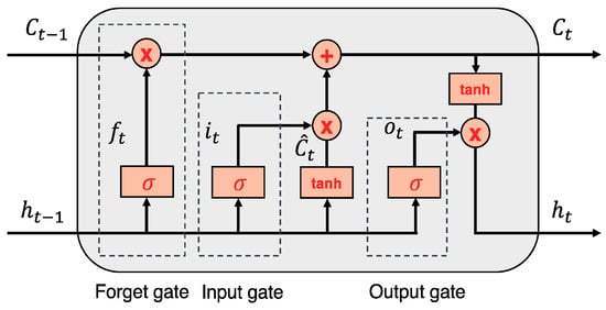
Figure 1.
LSTM architecture [32].
The outcome of this process ranges from 0 to 1, where 0 signifies full eradication of the value and 1 stands for preservation. The output gate ultimately selects which part of the LSTM memory will add to the output, utilizing a sigmoid layer to multiply the output of this layer with the non-linear tanh function which retains the values in the range of −1 to 1, according to the equations formulated in [38].
ot = σ(Woh[ht−1],Wox [xt], bo),
ht = ot ∗ tanh(ct),
2.2. Bi-LSTM
In the LSTM model, data is transmitted in one direction, conveying historical information [38]. Conversely, the Bi-LSTM model enables bi-directional data flow, transferring information about both the past and future. As a result, Bi-LSTM features two distinct hidden layers that are connected to the same input and output [39]. One of the hidden layers in Bi-LSTM consists of a forward LSTM that transfers historical data from the input sequence to the output sequence. Simultaneously, the other backward LSTM moves future data information from the output sequence to the input sequence. This mechanism enables the model to learn long-term dependencies and enhance its accuracy [40]. Bi-LSTM architecture is given in Figure 2. Here, the hidden state of Bi-LSTM at time t comprises forward and backward , while Ht denotes the final hidden output of Bi-LSTM, which results from combining the forward and backward outputs. Technical terms are explained upon their initial usage to ensure clarity [41]:
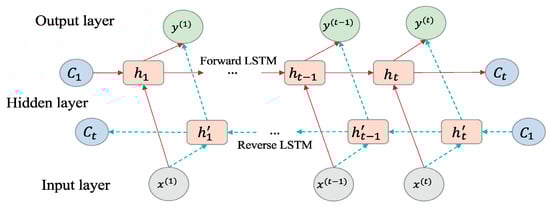
Figure 2.
Bi-LSTM architecture [32].
2.3. Attention Mechanism (AM)
AM can be explained by the perception mechanism in the human brain. The brain selects only necessary information from the outside world rather than perceiving all information at once. Similarly, in AM, attention weight is defined to prioritize important information and ignore irrelevant data. This process aims to give more attention to pertinent information. To map the first xt to ht in the AM process, use the following equation:
Here, f1 represents a non-linear activation function, ht stands for the hidden state at time t, and s denotes the size of hidden state. Additionally, the formulas mentioned below are employed to create an attention mechanism.
where , represents a sequence of features, denotes the previous hidden state in the LSTM unit, and Ct−1 refers to the prior cell state in the LSTM unit. The vector V, along with matrices W1 and W2, signify the model’s learnable parameters. The length of αk vector is m, and its ith item reveals the significance of the kth input feature sequence at time t. βk denotes an attention weight that contains an attention score for the kth feature sequence. The weighted input feature sequence zt can be derived as follows.
Afterwards, the initial input features of xt are substituted with the zt obtained from here, which leads to the update of the attention model. The end result of zt becomes the novel input of the LSTM-DL model. Thanks to the attention weight, redundant feature sequences can be excluded, while important input feature sequences can be emphasized. The model’s process flow is depicted in Figure 3 below [42].
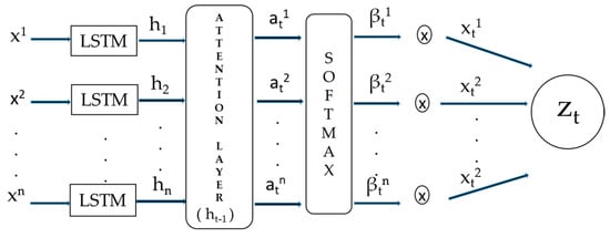
Figure 3.
Attention mechanism.
2.4. Feature Selection
Today, practitioners and researchers deal with large datasets comprised of hundreds, if not thousands, of features. In machine learning, variations in the target variable are primarily attributed to the initial input variables; however, their influence on the target variable may differ. Conversely, features that are either unrelated or highly correlated to the target variable can significantly compromise model performance. To address these challenges, practitioners utilize feature selection methods during the data pre-processing stage. Feature selection involves distinguishing relevant features from less important ones through dimensionality reduction techniques, ultimately enhancing model performance. Feature selection methods can be categorized into four groups for evaluating feature subsets: filter, wrapper, embedded, and hybrid methods. Filter methods assess feature relevance based on the dataset’s nature to produce a ranked list of all features, regardless of the estimator used. Technical abbreviations will be explained at their initial usage throughout the text. Filtering techniques include mutual information, PC, correlation coefficient, information gain, gain ratio, Laplacian score, Fisher score, chi-squared, correlation-based feature selection, fast correlation-based filter, constraint score, relief, minimal-redundancy-maximal-relevance. Meanwhile, wrappers determine the relevance of feature subsets based on their performance in model prediction using ML-DL. Any greedy search strategies, including branch-and-bound, simulated annealing, genetic algorithms, and any classifier algorithms, can be utilized to produce a wrapper method. Recursive feature elimination (RFE) and Boruta algorithm are both examples of wrapper methods. RFE is a well-known and effective feature selection algorithm as a wrapper, which is easy to set up and utilize, and capable of identifying more relevant features in a training dataset. The random forest classification model is used to rank features based on their importance using a recursive method [43]. Built-in components of certain ML algorithms, embedded feature selection methods, rank features during the model’s training phase. Tree-based algorithms such as decision trees, random forests, and gradient boosting are some examples of these methods [44]. On the other hand, nearly any filter, wrapper, or embedded technique can be integrated into a multi-step operation to create a hybrid approach that utilizes the strengths of each method. By applying the filter step in a hybrid approach, the feature search space is reduced, facilitating the use of computationally expensive wrapper or embedded methods for high-dimensional datasets [45].
2.5. Introduction to XAI and LIME
Although deep learning methods provide significant advancements and yield positive outcomes in various fields, the lack of interpretability due to their black-box structure could hinder practitioners from adopting them. Henceforth, the literature in recent years has seen a significant number of studies proposing XAI techniques to elucidate the decision-making process of deep learning models. Although interpretability can be classified in various ways, it is generally analyzed through two categories: intrinsic interpretability and post-hoc explanations.
Intrinsic interpretability approaches aim to create DL models that are transparent. However, post-hoc methods utilize techniques like feature attribution methods, textual explanations, and visualizations to explain the behavior of black-box models, which are opaque DL models. There are two ways to examine post-hoc explanations: model-agnostic and model-specific explanations. Model-specific explanations are limited to particular models, with the embedded feature importance function of tree-based models being the most well-known. Conversely, model-agnostic approaches are not dependent on a specific model and can be applied to any type of model. Post hoc model-agnostic approaches, which aim to develop an algorithm to explain the decision-making process of a DL model, are generally preferred over other approaches in practice. In terms of scope, XAI methods can provide either global or local explanations. For the purpose of this discussion, we will focus solely on local explanations. LIME, a notable model-agnostic algorithm, elucidates forecasts by replacing complex models with a locally interpretable surrogate model [46]. Locally interpretable surrogate models can be formulated as follows:
Here, G represents the overall potential linear regression model while g is the instance (x)-specific explanation model. The goal of model g is to minimize loss L which measures its proximity to the prediction of the actual f model. Moreover, Ω(g) is responsible for keeping the complexity of the model low in the above formula. πx represents a measure of proximity that describes the size of the neighborhood surrounding the instance x for explanation purposes. In practice, the user must specify the complexity of LIME by choosing the maximum number of features that can be used by the linear regression model, since LIME solely optimizes the loss.
2.6. Model Performance Evaluation Metrics
Several metrics are utilized to evaluate the accuracy of forecasting results in scientific research. In this study, we assessed our predictions using two commonly employed metrics: root mean square error (RMSE) and mean absolute percentage error (MAPE). The following formulas depict these metrics.
where n is the data number in total; yi is the actual load value and is the forecasted load value at time t.
3. Methodology
3.1. Exploratory Data Analysis
3.1.1. Data Integrity and Visualization
The dataset aggregates data from diverse load types in Australia, covering dates ranging from 1 January 2006 to 1 January 2011. It comprises six distinct features, namely electrical load consumption (‘SYSLoad’), the dry bulb temperature (‘DryBulb’), the dew point temperature (‘DewPnt’), the dry bulb temperature (‘WetBulb’), humidity, and electricity price (‘ElecPrice’). The target variable is the electrical load consumption values, represented by ‘SYSLoad’. All variables, except for ‘ElecPrice’ depict the climatic information. ‘ElecPrice’ can be obtained from the Australian Electricity Market Operator (AEMO).
Before performing a time series analysis, it is necessary to evaluate whether the data are stationary or not. The fact that the data is not stationary indicates that the prediction model cannot adequately detect the basic points in the data and that the results obtained are likely to have an error rate. For this reason, the stationarity of the used dataset was tested using the Augmented Dickey–Fuller test statistical method. The statistical values obtained as a result of this test are shown in Figure 4, Table 1. If the p-value is less than 0.05, it means that the null hypothesis is rejected. This proves that the dataset used is stationary.
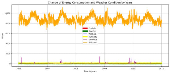
Figure 4.
Line plot of daily total electrical load consumption from 2006 to 2011.

Table 1.
Augmented Dickey–Fuller test result.
Since the goal of the study was to estimate the medium-term (one month ahead) load, the half-hourly load data were first converted to daily data. At this stage, the sum of all values of each characteristic for a day was resampled and 1827 days of load observation data were obtained. In order to obtain a more stable prediction result, the data to be processed by the model must have integrity and be normalized. For this purpose, the data used was first checked for null fields and it was found that there were no missing data. To visualize the dataset, Figure 4 and Figure 5 show the change in electricity consumption over the years based on all features and each feature in the dataset, respectively.
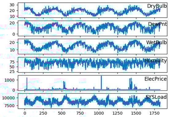
Figure 5.
Line plot of daily total electrical load consumption for 1827 days on a feature basis.
3.1.2. Feature Engineering
In the first version of the dataset used, there are six features: ‘DryBulb’, ‘DewPnt’, ‘WetBulb’, ‘Humidity’, ‘ElecPrice’, and ‘SYSLoad’. The k-fold cross-validation method, a validation strategy, was used to determine whether the number of existing features is sufficient for the model to make highly accurate predictions, in other words, to determine to what extent the addition of new features may affect the performance of the model. For this purpose, the model was first trained with the RFR, ML algorithm using the six-feature version of the dataset, and the root mean squared log error (RMSLE) of the model was calculated to be 0.06. Then, the model was trained with the RFR algorithm by adding three new features, ‘day of the month’, ‘day of the week’, and ‘hour of the day’ to the existing dataset. As a result, the RMSLE value was calculated to be 0.04. Since the error level was only reduced by 0.02, it was decided that adding new features would not significantly improve the prediction result. On the other hand, in time series estimation, it is preferred to go back to the determined day, hour, etc. value (i.e., lagged values) and make predictions for the future values based on these historical values. Accordingly, the prediction accuracy of the model was examined by considering the 30-day lag for all input features, which is the most preferred in MTLF.
3.1.3. Evolution of Feature Importance and Extraction of Irrelevant Features
Before training the regression model, an investigation was made to determine how many features were needed in the dataset. The process of identifying important features and removing features considered unnecessary was performed to avoid increasing the computational time and model complexity of the regression model and to avoid overfitting. In other words, the goal of the model is to learn only the necessary features and not be exposed to unnecessary or noisy data. Therefore, the relationship between the input features and the relative variable ‘SYSLoad’ feature was first examined using PC. At this stage, 0.25 was chosen as the threshold value and it was found that the input variables that were above the threshold value and had the highest correlation with the target variable (‘SYSLoad’) were ‘DryBulb’, ‘WetBulb’, ‘ElecPrice’. Figure 6 and Figure 7 show the results of the PC analysis.
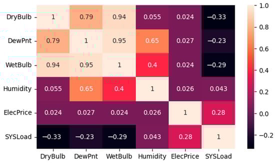
Figure 6.
PC analysis results.
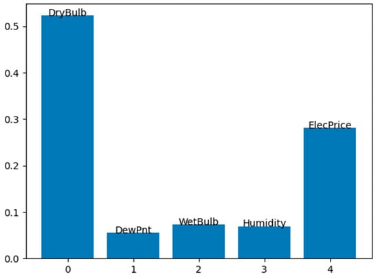
Figure 7.
Features’ importance as a result of the implementation of the RFR and DTR algorithms.
In order to prove the effectiveness of the three input features mentioned above, which are considered to be the most effective as a result of the PC analysis, the features were ranked in order of importance using the RFR and DTR algorithms. Figure 7 and Figure 8 shows the importance ranking of all the features. The RFECV method was then applied to ensure that the model automatically selected the ideal number of features. As a result of all these sorting and selection processes, the features ‘DryBulb’, ‘WetBulb’ and ‘ElecPrice’ were determined to be the most effective features, just as in the PC analysis.
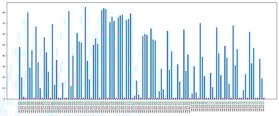
Figure 8.
The most effective lag values among all lag values for training of the model.
Time lag for features was implemented for the ‘DryBulb’, ‘WetBulb’, ‘ElecPrice’, and ‘SYSLoad’ features from the previous feature selection step. Accordingly, the values of each of the four features from 30 days ago to time t and the values of the target variable, the ‘SYSLoad’ variable, from time t to 30 days later became the new features to feed into the model. The number of these features, in other words the number of columns, was found to be 150 (120 input, 30 target) features. However, since the number of 120 input features would increase the computation time of the model and cause the complexity of the model, the RFECV method was applied again and the most necessary features were determined, as a result, the 120 input features were reduced to 36. Therefore, as a result of the selection of important lags, the number of input features to be given to the models used was obtained as 36. Figure 8 shows a bar chart of the final lag values fed to the model, and the short bars indicate the most effective lag values among all the lag values. In this figure, var1: DryBulb, var2: WetBulb, var3: ElecPrice, and var4: SYSLoad, and the short bars indicate the most effective lag values among all lag values.
3.2. Model Architecture
In the study, three different model architectures were created. The first is Model1, which is the Bi-LSTM model, the second is Model2, which has the LSTM architecture, and the last is Model3, in which the custom attention layer is added to the LSTM architecture.
Model1 has a Bi-LSTM layer and a dense layer following it. In addition, a dropout layer was added between each Bi-LSTM layer to reduce overfitting. The number of neurons and epochs in the Bi-LSTM layers are 512 and 60, respectively. The batch size is 72, the learning rate is 0.0001, the dropout is 0.2, and the optimizer is Adam. The activation function is linear activation and the loss function is mean absolute error (MAE). The mean squared error (MSE) was used as the validation metric of the model. Seventy-five (75)% of the dataset was reserved for training and 25% for testing. Model2 is the LSTM applied version of Model1. In Model3, the custom attention layer from the Keras library was added after the LSTM layer. The attention layer consists of two dense layers. The hyperparameter settings of the three separate models are shown in Table 2.
Table 2.
Hyperparameter settings for three separate models.
3.3. Experimental Setup
This study was divided into three separate sub-study groups according to certain input characteristics, and all models (Model1, Model2, and Model3) were trained accordingly. This section provides information on how Subset1, Subset2, and Subset3 were created for this study.
3.3.1. Training with Subset1
The study is aimed to examine how the selection of features and lag value would change the error rate of the model. To do so, each model created was first trained using the first features (five input, one output) without making any feature selection. Accordingly, the value of each input feature from 30 days ago constituted the input data of the models.
3.3.2. Training with Subset2
At this stage, as a result of applying the feature selection methods specified in Section 3.1.3, PC, RFR, DTR and RFECV, the five features initially included in the dataset have been reduced to three features. These selected features are ‘DryBulb’, ‘WetBulb’, ‘ElecPrice’ and represent the input values, ‘SYSLoad’ represents the target variable. For this dataset, the time-delayed value of each input feature for 30 days constituted the input data to the models.
3.3.3. Training with Subset3
The 30-day lagged values of the ‘DryBulb’, ‘WetBulb’, ‘ElecPrice’, and ‘SYSLoad’ features, which were determined to be the most important in the third dataset, were obtained by transforming the time series into supervised learning. As a result of this process, 120 input features and 30 output features were obtained. However, since it was thought that 120 input features could increase the complexity of each model and prolong the training time, an attempt was made to determine the most effective among the 120 lagged feature values using the RFECV method. As a result, the number of input features was reduced from 120 to 36. Therefore, a data frame with 36 input and 30 output features was obtained.
4. Experimental Results
In order to measure the average performance of the models, a cross-validation (CV) process was applied to each model, dividing the time series data into 10 parts. The average MAPE and RMSE values obtained after this process are all included here.
4.1. Results of Subset1
The results of the performance metrics obtained as a result of training the three models using the Subset1 dataset are presented in Table 3. It can be seen from the table that the RMSE and MAPE results of all the models are quite low, in other words, the prediction results and the actual values are very close to each other. Among these models, Model2, which is based on the LSTM architecture, has the lowest error.
Table 3.
Results of Subset1.
Figure 9 shows the one-month-ahead prediction results of Model1, Model2, and Model3, respectively, for test data in the Subset1 dataset. In this figure, the blue and orange lines indicate the actual load values and the predicted values, respectively. By analyzing the figure, it can be inferred that Model2 provides the best approximation of the actual load value using the Subset1 test data.
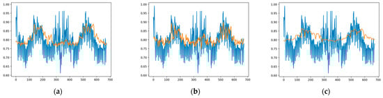
Figure 9.
Forecasting results of the models based on subset1: (a) Model1 results; (b) Model2 results; (c) Model3 results.
In the study, LIME values are explained using RecurrentTabularExplainer. The local explanation of the LIME method is made on the scaled data, as is the actual model’s prediction. Figure 10 shows the LIME results of Model1, Model2, and Model3, respectively, using the Subset1 dataset. As can be seen from the graphs, the output of the LIME method consists of three stages. Accordingly, the progress bar on the left in Figure 10 shows the changing range of the resulting estimated ‘SYSLoad’ value. While the bar chart in the middle part of the figure shows the features that contribute positively and negatively to the prediction. The features in the bar chart in the middle of the figure are determined by LIME, and these features are selected among the features that have the most positive and negative impact on the prediction for the relevant sample, the table on the far right of the figure gives the list of the actual feature values. In this list on the right side of the figure for all models, feature values colored in orange indicate that they have a positive impact on the prediction value, while feature values colored in blue have a negative impact. The XAI results in that figure are from the fifth test instance for Model1, and from the second test instance for Model2 and Model3. Looking at the LIME results evaluated for the randomly selected instance for Model1 in the figure, we see that the prediction of the ‘SYSLoad’ value made by this model for the fifth sample is 0.8, and the min-max range varies between 0.76 and 0.83. For Model1, the lagged values of the ‘DryBulb’ feature for 5, 6, 7, 8, 10, 11, 12, and 13 days prior had a negative effect on the prediction value by obtaining a value less than 0.67, while the value of the “Humidity” feature for the current and one day lagged contributed positively by obtaining a value more than 0.74. This means that a ‘Humidity’ value greater than 0.74 had a positive effect on the prediction result, but a ‘DryBulb’ value greater than 0.67 had a negative effect on it. These values are different for each other feature as seen in the bar chart in the middle of the figure, and what determines this is the application of the LIME approach to the model. For Model1, the feature values in the list on the far right of the figure enable the model to produce an XAI prediction score of 0.80. In short, summarizing these results for Model1, the more lagged values of the ‘DryBulb’ feature have a negative impact on the model’s prediction, but the more recent lagged values of the ‘Humidity’ feature make a positive contribution to the prediction. From the figure for Model2, we can see that the predicted ‘SYSLoad’ value for the second sample is 0.78, and the min-max range varies between 0.74 and 0.82. According to the list on the right side of the figure for Model2, the values of the ‘ElecPrice’ feature of the 10-day lagged (ElecPrice_t-10) and the current value provide the most support for the accurate prediction of Model2. The one-day lagged, two-day lagged and the current value of the ‘DewPnt’ feature is 0.83, and this value, which is greater than 0.74, improves Model2’s prediction performance. The progress bar given on the left of the figure for Model3 shows that the prediction result of the model is 0.80. According to the list on the right side of the figure for Model3, the lagged values of the ‘DryBulb’ feature until the 14th day negatively affect the model prediction score. In summary, for Subset1, where no feature selection was made, the variables ‘Humidity’, ‘DewPnt’, ‘ElecPrice’ strengthen the prediction performance of the models.
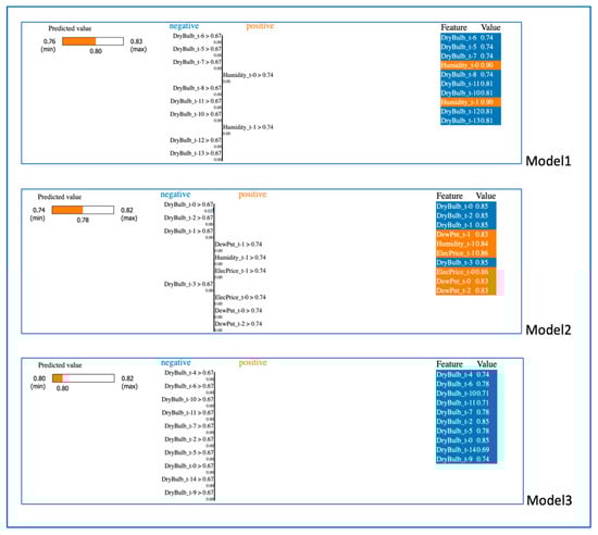
Figure 10.
LIME results of Model1, Model2 and Model3 by using subset1 dataset.
4.2. Results of Subset2
Table 4 shows the details of the performance results of all the models using the Subset2 dataset. Accordingly, the model with the lowest RMSE and MAPE results is Model1, which is based on the Bi-LSTM architecture. However, it is noticeable that Model2 and Model3 perform very similarly to Model1 according to the performance metrics.
Table 4.
Results of Subset2.
Figure 11 shows a graph of the one-month-ahead prediction of Model1, Model2, and Model3, respectively, this time with the test data in the Subset2 dataset. Examining this graph, we can see that the models that can best predict the actual load values are Model1 and Model2, and among them, the most ideal model in terms of its closeness to the actual value is Model1. The difference in RMSE and MAPE values between Model1 and Model2 in Table 3 also confirms this.
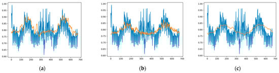
Figure 11.
Forecasting results of the models based on subset2: (a) Model1 results; (b) Model2 results; (c) Model3 results.
Figure 12 shows a visualization of the results of LIME when Model1, Model2, and Model3 use Subset2, respectively. The XAI results for Subset2 in the figure were obtained using the random second sample in the test set for all models. Looking at the results of Model1 here, we can see that the prediction score of Model1 is 0.79 and the parameters that have a positive effect on this score are the lagged values for the 27th, 28th and 29th days of ‘ElecPrice’ and the lagged values for the 28th and 29th days of ‘DryBulb’. In addition, recent lagged time values of ‘DryBulb’, ‘ElecPrice’ and ‘WetBulb’ negatively affect the prediction of the model. It can be seen that the prediction result for Model2 is 0.78, and while the lagged values for the 1st and 23rd day of ‘ElecPrice’ have a positive effect on the result, the lagged values of the remaining variables colored in blue on the right side of the figure for Model2 have a negative effect. For Model3, the predictive score is 0.77, and all of the variables listed on the right side contribute negatively to the model reaching this minimum predictive score. Summarizing the overall situation for Subset2, where three features were selected from the first five features of the dataset and prepared by taking all the lagged values of these features up to 30 days, it can be inferred that determining the lagging range based on 30 days is the right step because the lagged values of the selected features going back further strengthen the prediction of the models. In addition, ‘DryBulb’ and ‘ElecPrice’, which are the most effective features for Subset2, improve the model in real terms, so an effective feature selection can be achieved.
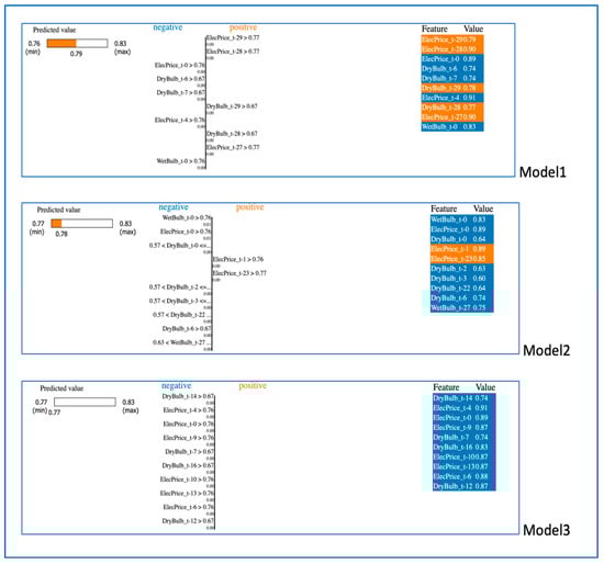
Figure 12.
LIME results of Model1, Model2 and Model3 by using subset2 dataset.
4.3. Results of Subset3
Table 5 shows the RMSE and MAPE results obtained for Subset3. It can be seen from the table that these results are lower for Model1 and Model2 than for Model3. When Model1 and Model2 are compared, it can be seen that Model1 has more successful results in terms of RMSE and MAPE values.
Table 5.
Results of Subset3.
In Figure 13, a graph is given showing the prediction of 30 days-ahead by applying Model1, Model2, and Model3, respectively, using Subset3. If these results are compared between models, it is seen that the closest approach to the real load value for Subset3 is achieved by Model1, and the results in Table 4 confirm that.
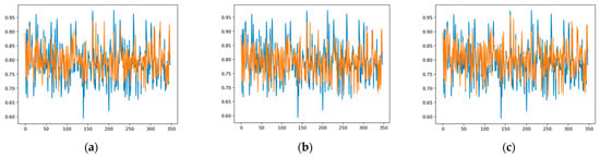
Figure 13.
Forecasting results of the models based on Subset3: (a) Model1 results; (b) Model2 results; (c) Model3 results.
Figure 14 shows a visualization of the LIME results of the predictions made with Model1, Model2, and Model3, respectively, using Subset3. The XAI results for Subset3 were obtained using a random first sample in the test set for all models. As can be seen from the LIME results, the prediction of Model1 is 0.89, and many time-lagged values of the ‘SYSLoad’ feature and a one-day lagged value of the ‘DryBulb (t-1)’ feature in the right figure contribute positively to the prediction score. The predictive value of Model2 is 0.88, and as in Model1, the ‘DryBulb’ and ‘SYSLoad’ features have a positive impact on this prediction result. While the values of the ‘DryBulb (t-1)’, ‘SYSLoad (t-20)’, ‘SYSLoad (t-13)’, ‘DryBulb (t-7)’ features positively improve the prediction of Model2, the ‘SYSLoad (t-17)’ and ‘SYSLoad (t-18)’ features have a negative effect. The prediction value of Model3 is 0.90, and the features that contribute positively to this model are the values of the ‘DryBulb’ and ‘SYSLoad’ features, as in Model1 and Model2. As shown in the table, the values of ‘SYSLoad (t-13)’, ‘SYSLoad (t-5)’, ‘SYSLoad (t-6)’, ‘SYSLoad (t-7)’, ‘SYSLoad (t-13)’, and ‘SYSLoad (t-20)’ contributed the most to the prediction of Model3. When the XAI results from Subset3 are evaluated on a feature basis, it can be inferred that the most effective features are ‘SYSLoad’ and ‘DryBulb’.
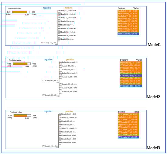
Figure 14.
LIME results of Model1, Model2 and Model3 by using the Subset3 dataset.
In addition, among the features used for all subsets, the lagged values of the features generally close to 30 days contribute positively to the prediction of the models. This shows that all the feature selection processes performed in the feature engineering and time-lagged up to 30 days are correct and useful processes in terms of this study.
5. Conclusions
Within the framework of ELF, which is an indispensable part of power system planning and management studies, many studies have been carried out for various load types regarding short-term load forecasting, and while very successful forecasting results can be obtained, the number of studies in the literature regarding medium-term and long-term load forecasting is much smaller. The accuracy of forecasting results for these time periods is relatively lower depending on the length of the time horizon to be forecasted. In this context, the main objective of this study was to improve the medium-term electric load forecasting with certain approaches, models and techniques. To this end, the aggregated load dataset and its features were first analyzed through EDA and feature engineering. Multivariate medium-term ELF was performed separately with LSTM, Bi-LSTM, and attention-based LSTM approaches, which are among the most successful models in ELF. LIME, a post hoc model agnostic approach, was applied to these models based on DL, and the effects of the features of the datasets on the prediction results obtained could be interpreted.
- As part of the EDA, the stationarity of the aggregated load data was tested using the Augmented Dickey–Fuller statistical test method, and the statistical measures obtained as a result showed that the dataset was stationary.
- The correlation and importance of each feature was determined using the hybrid framework developed in feature engineering. Accordingly, ‘DryBulb’, ‘WetBulb’ and ‘ElecPrice’ were selected as the three most important features among the previous five features of the dataset by the combined feature selection approaches.
- Since this is a month-ahead load forecast, all forecast models have been trained with the time lags of all characteristics up to 30 days ago.
- Comparative results of three different subsets created to study the effect of the selected features and the determined time delay values on the models are shown in Table 6 and Figure 15 below. It can be seen from the table that the RMSE and MAPE values are highest in Subset1, where all features are present, obtaining 0.074 and 0.077, respectively, while the values of these metrics decrease by more than 20% in Subset2, which is obtained by selecting only the most effective features. In Subset3, where the most effective features have been obtained by selecting the most important time lags of the features, the RMSE and MAPE results have the lowest values of 0.046 and 0.044, respectively. There is a decrease of more than 40% in the prediction error measurements compared to Subset1 with the use of Subset3.
Table 6. Overall metric results based on subsets.
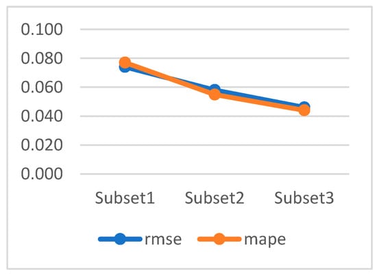 Figure 15. Graphical representation of performance results by subsets.
In this study, a significant improvement was achieved in terms of prediction model performance. Based on this point, it can be concluded that feature selection is effective for this study in improving model performance and prediction accuracy, and retraining by selecting important lag features is a correct strategy. Quantitative and detailed evaluations have been conducted, and experimental results show that this entire solution approach is fully successful for multivariate medium-term aggregated load forecasting.
Our forward-looking studies will primarily be carried out to develop medium- and long-term load forecasting, which has not been studied much in the literature so far. In this direction, we plan to work on the development of DL approaches and ensemble DL architectures. However, we also plan to develop feature engineering studies considering the results obtained with XAI. We also considered that the time delay value for the features can be obtained with the help of optimization techniques.
Author Contributions
Conceptualization, F.Y. and M.V.A.; methodology, F.Y. and M.V.A.; software, M.V.A.; validation, F.Y. and M.V.A.; formal analysis, F.Y. and M.V.A.; investigation, F.Y. and M.V.A.; resources, F.Y. and M.V.A.; data curation, M.V.A.; writing—original draft preparation, F.Y.; writing—review and editing, F.Y.; visualization, F.Y. and M.V.A.; supervision, F.Y. and M.V.A. All authors have read and agreed to the published version of the manuscript.
Funding
This research received no external funding.
Institutional Review Board Statement
Not applicable.
Informed Consent Statement
Not applicable.
Data Availability Statement
The data set used is a table of historical hourly loads and temperature observations from the AEMO & BOM for Sydney/NSW for the years 2006 to 2010. This data was accessed via Matlab official website: https://www.mathworks.com/matlabcentral/fileexchange/31877-electricity-load-forecasting-for-the-australian-market-case-study?s_tid=srchtitle_site_search_7_electrical%20load%20forecasting.
Conflicts of Interest
The authors declare no conflict of interest.
References
- Dudek, G.; Pełka, P. Pattern Similarity-Based Machine Learning Methods for Mid-Term Load Forecasting: A Comparative Study. Appl. Soft Comput. 2021, 104, 107223. [Google Scholar] [CrossRef]
- Liu, H.; Yu, C.; Yu, C. A new hybrid model based on secondary decomposition, reinforcement learning and SRU network for wind turbine gearbox oil temperature forecasting. Measurement 2021, 178, 109347. [Google Scholar] [CrossRef]
- Yan, G.; Yu, C.; Bai, Y. A New Hybrid Ensemble Deep Learning Model for Train Axle Temperature Short Term Forecasting. Machines 2021, 9, 312. [Google Scholar] [CrossRef]
- Yu, C.; Wang, F.; Shao, Z.; Sun, T.; Wu, L.; Xu, Y. DSformer: A Double Sampling Transformer for Multivariate Time Series Long-term Prediction. In Proceedings of the 32nd ACM International Conference on Information and Knowledge Management, Birmingham, UK, 21–25 October 2023. [Google Scholar]
- Hirose, K. Interpretable Modeling for Short- and Medium-Term Electricity Demand Forecasting. Front. Energy Res. 2021, 9, 724780. [Google Scholar] [CrossRef]
- Oreshkin, B.N.; Dudek, G.; Pełka, P.; Turkina, E. N-BEATS Neural Network for Mid-Term Electricity Load Forecasting. Appl. Energy 2021, 293, 116918. [Google Scholar] [CrossRef]
- Smyl, S. A Hybrid Method of Exponential Smoothing and Recurrent Neural Networks for Time Series Forecasting. Int. J. Forecast. 2020, 36, 75–85. [Google Scholar] [CrossRef]
- Son, N.; Yang, S.; Na, J. Deep Neural Network and Long Short-Term Memory for Electric Power Load Forecasting. Appl. Sci. 2020, 10, 6489. [Google Scholar] [CrossRef]
- Shirzadi, N.; Nizami, A.; Khazen, M.; Nik-Bakht, M. Medium-Term Regional Electricity Load Forecasting through Machine Learning and Deep Learning. Designs 2021, 5, 27. [Google Scholar] [CrossRef]
- Bouktif, S.; Fiaz, A.; Ouni, A.; Serhani, M.A. Optimal Deep Learning LSTM Model for Electric Load Forecasting Using Feature Selection and Genetic Algorithm: Comparison with Machine Learning Approaches. Energies 2018, 11, 1636. [Google Scholar] [CrossRef]
- Bouktif, S.; Fiaz, A.; Ouni, A.; Serhani, M.A. Single and Multi-Sequence Deep Learning Models for Short and Medium Term Electric Load Forecasting. Energies 2019, 12, 149. [Google Scholar] [CrossRef]
- Masood, Z.; Gantassi, R.; Ardiansyah; Choi, Y. A Multi-Step Time-Series Clustering-Based Seq2Seq LSTM Learning for a Single Household Electricity Load Forecasting. Energies 2022, 15, 2623. [Google Scholar] [CrossRef]
- Cho, J.; Yoon, Y.; Son, Y.; Kim, H.; Ryu, H.; Jang, G. A Study on Load Forecasting of Distribution Line Based on Ensemble Learning for Mid-to Long-Term Distribution Planning. Energies 2022, 15, 2987. [Google Scholar] [CrossRef]
- Kumar, S.; Hussain, L.; Banarjee, S.; Reza, M.; Tech, B.; Students, Y. Energy Load Forecasting Using Deep Learning Approach-LSTM and GRU in Spark Cluster. In Proceedings of the Fifth International Conference on Emerging Applications of Information Technology (EAIT), Kolkata, India, 12–13 January 2018; pp. 1–4. [Google Scholar]
- Han, L.; Peng, Y.; Li, Y.; Yong, B.; Zhou, Q.; Shu, L. Enhanced Deep Networks for Short-Term and Medium-Term Load Forecasting. IEEE Access 2019, 7, 4045–4055. [Google Scholar] [CrossRef]
- Khalid, A.; Abbas, S.; Iqbal, S. Deep LSTM-BiGRU Model for Electricity Load and Price Forecasting in Smart Grids Deep LSTM-BiGRU Model for Electrcity Load and Price Forecasting in Smart Grids. EasyChair Prepr. 2022, 8663. Available online: https://easychair.org/publications/preprint/NcTd (accessed on 29 October 2023).
- Jin, B.; Zeng, G.; Lu, Z.; Peng, H.; Luo, S.; Yang, X.; Zhu, H.; Liu, M. Hybrid LSTM–BPNN-to-BPNN Model Considering Multi-Source Information for Forecasting Medium- and Long-Term Electricity Peak Load. Energies 2022, 15, 7584. [Google Scholar] [CrossRef]
- Cheng, Z.; Wang, L.; Yang, Y. A Hybrid Feature Pyramid CNN-LSTM Model with Seasonal Inflection Month Correction for Medium- and Long-Term Power Load Forecasting. Energies 2023, 16, 3081. [Google Scholar] [CrossRef]
- Gul, M.J.; Urfa, G.M.; Paul, A.; Moon, J.; Rho, S.; Hwang, E. Mid-Term Electricity Load Prediction Using CNN and Bi-LSTM. J. Supercomput. 2021, 77, 10942–10958. [Google Scholar] [CrossRef]
- Sehovac, L.; Grolinger, K. Deep Learning for Load Forecasting: Sequence to Sequence Recurrent Neural Networks with Attention. IEEE Access 2020, 8, 36411–36426. [Google Scholar] [CrossRef]
- Xu, H.; Fan, G.; Kuang, G.; Song, Y. Construction and Application of Short-Term and Mid-Term Power System Load Forecasting Model Based on Hybrid Deep Learning. IEEE Access 2023, 11, 37494–37507. [Google Scholar] [CrossRef]
- Butt, F.M.; Hussain, L.; Jafri, S.H.M.; Alshahrani, H.M.; Al-Wesabi, F.N.; Lone, K.J.; El Din, E.M.T.; Duhayyim, M.A. Intelligence Based Accurate Medium and Long Term Load Forecasting System. Appl. Artif. Intell. 2022, 36, 2088452. [Google Scholar] [CrossRef]
- Zhang, S.; Chen, R.; Cao, J.; Tan, J. A CNN and LSTM-Based Multi-Task Learning Architecture for Short and Medium-Term Electricity Load Forecasting. Electr. Power Syst. Res. 2023, 222, 109507. [Google Scholar] [CrossRef]
- Liapis, C.M.; Karanikola, A.; Kotsiantis, S. A Multivariate Ensemble Learning Method for Medium-Term Energy Forecasting. Neural Comput. Appl. 2023, 35, 21479–21497. [Google Scholar] [CrossRef]
- Yaprakdal, F.; Bal, F. Comparison of Robust Machine-Learning and Deep-Learning Models for Midterm Electrical Load Forecasting. Eur. J. Tech. 2022, 12, 102–107. [Google Scholar] [CrossRef]
- Cordeiro-Costas, M.; Villanueva, D.; Eguía-Oller, P.; Martínez-Comesaña, M.; Ramos, S. Load Forecasting with Machine Learning and Deep Learning Methods. Appl. Sci. 2023, 13, 7933. [Google Scholar] [CrossRef]
- Ayub, N.; Irfan, M.; Awais, M.; Ali, U.; Ali, T.; Hamdi, M.; Alghamdi, A.; Muhammad, F. Big Data Analytics for Short and Medium-Term Electricity Load Forecasting Using an AI Techniques Ensembler. Energies 2020, 13, 5193. [Google Scholar] [CrossRef]
- Ahmad, T.; Zhang, H. Novel Deep Supervised ML Models with Feature Selection Approach for Large-Scale Utilities and Buildings Short and Medium-Term Load Requirement Forecasts. Energy 2020, 209, 118477. [Google Scholar] [CrossRef]
- Hu, Z.; Bao, Y.; Chiong, R.; Xiong, T. Mid-Term Interval Load Forecasting Using Multi-Output Support Vector Regression with a Memetic Algorithm for Feature Selection. Energy 2015, 84, 419–431. [Google Scholar] [CrossRef]
- Machlev, R.; Heistrene, L.; Perl, M.; Levy, K.Y.; Belikov, J.; Mannor, S.; Levron, Y. Explainable Artificial Intelligence (XAI) Techniques for Energy and Power Systems: Review, Challenges and Opportunities. Energy AI 2022, 9, 100169. [Google Scholar] [CrossRef]
- Gürses-Tran, G.; Körner, T.A.; Monti, A. Introducing Explainability in Sequence-to-Sequence Learning for Short-Term Load Forecasting. Electr. Power Syst. Res. 2022, 212, 108366. [Google Scholar] [CrossRef]
- Mouakher, A.; Inoubli, W.; Ounoughi, C.; Ko, A. EXPECT: EXplainable Prediction Model for Energy ConsumpTion. Mathematics 2022, 10, 248. [Google Scholar] [CrossRef]
- Kim, J.Y.; Cho, S.B. Explainable Prediction of Electric Energy Demand Using a Deep Autoencoder with Interpretable Latent Space. Expert. Syst. Appl. 2021, 186, 115842. [Google Scholar] [CrossRef]
- Moon, J.; Rho, S.; Baik, S.W. Toward Explainable Electrical Load Forecasting of Buildings: A Comparative Study of Tree-Based Ensemble Methods with Shapley Values. Sustain. Energy Technol. Assess. 2022, 54, 102888. [Google Scholar] [CrossRef]
- Chen, Y.; Fu, Z. Multi-Step Ahead Forecasting of the Energy Consumed by the Residential and Commercial Sectors in the United States Based on a Hybrid CNN-BiLSTM Model. Sustainability 2023, 15, 1895. [Google Scholar] [CrossRef]
- Freeborough, W.; van Zyl, T. Investigating Explainability Methods in Recurrent Neural Network Architectures for Financial Time Series Data. Appl. Sci. 2022, 12, 1427. [Google Scholar] [CrossRef]
- Hochreiter, S.; Schmidhuber, J. Long Short-term Memory. Neural Comput. 1997, 9, 1735–1780. [Google Scholar] [CrossRef]
- Reddybattula, K.D.; Nelapudi, L.S.; Moses, M.; Devanaboyina, V.R.; Ali, M.A.; Jamjareegulgarn, P.; Panda, S.K. Ionospheric TEC Forecasting over an Indian Low Latitude Location Using Long Short-Term Memory (LSTM) Deep Learning Network. Universe 2022, 8, 562. [Google Scholar] [CrossRef]
- Vankadara, R.K.; Mosses, M.; Siddiqui, M.I.H.; Ansari, K.; Panda, S.K. Ionospheric Total Electron Content Forecasting at a Low-Latitude Indian Location Using a Bi-Long Short-Term Memory Deep Learning Approach. IEEE Trans. Plasma Sci. 2023, 1–11. [Google Scholar] [CrossRef]
- Shahin, A.I.; Almotairi, S. A Deep Learning BiLSTM Encoding-Decoding Model for COVID-19 Pandemic Spread Forecasting. Fractal Fract. 2021, 5, 175. [Google Scholar] [CrossRef]
- Wang, S.; Wang, X.; Wang, S.; Wang, D. Bi-Directional Long Short-Term Memory Method Based on Attention Mechanism and Rolling Update for Short-Term Load Forecasting. Int. J. Electr. Power Energy Syst. 2019, 109, 470–479. [Google Scholar] [CrossRef]
- Zhang, X.; Liang, X.; Zhiyuli, A.; Zhang, S.; Xu, R.; Wu, B. AT-LSTM: An Attention-Based LSTM Model for Financial Time Series Prediction. IOP Conf. Ser. Mater. Sci. Eng. 2019, 569, 052037. [Google Scholar] [CrossRef]
- Islam, M.R.; Lima, A.A.; Das, S.C.; Mridha, M.F.; Prodeep, A.R.; Watanobe, Y. A Comprehensive Survey on the Process, Methods, Evaluation, and Challenges of Feature Selection. IEEE Access 2022, 10, 99595–99632. [Google Scholar] [CrossRef]
- Zacharias, J.; von Zahn, M.; Chen, J.; Hinz, O. Designing a Feature Selection Method Based on Explainable Artificial Intelligence. Electron. Mark. 2022, 32, 2159–2184. [Google Scholar] [CrossRef]
- Pudjihartono, N.; Fadason, T.; Kempa-Liehr, A.W.; O’Sullivan, J.M. A Review of Feature Selection Methods for Machine Learning-Based Disease Risk Prediction. Front. Bioinform. 2022, 2, 927312. [Google Scholar] [CrossRef] [PubMed]
- Zafar, M.R.; Khan, N. Deterministic Local Interpretable Model-Agnostic Explanations for Stable Explainability. Mach. Learn. Knowl. Extr. 2021, 3, 521–545. [Google Scholar] [CrossRef]
Disclaimer/Publisher’s Note: The statements, opinions and data contained in all publications are solely those of the individual author(s) and contributor(s) and not of MDPI and/or the editor(s). MDPI and/or the editor(s) disclaim responsibility for any injury to people or property resulting from any ideas, methods, instructions or products referred to in the content. |
© 2023 by the authors. Licensee MDPI, Basel, Switzerland. This article is an open access article distributed under the terms and conditions of the Creative Commons Attribution (CC BY) license (https://creativecommons.org/licenses/by/4.0/).