Infinite Series Based on Bessel Zeros

Abstract

An interesting series based on Bessel function roots (zeros) is discussed and numerically analyzed. The novel-derived simplified general solutions are based on Lommel polynomials. This kind of series can have a large practical use in many scientific areas, such as solid mechanics, fluid mechanics, thermodynamics, electronics, physics, etc. Some practical examples connected with fluid mechanics are provided in this paper. The errors in Afanasiev solutions are corrected. In addition, the main solution for the series analyzed by Baricz and Angel is presented.

1. Introduction

Rayleigh series [1] (also called Rayleigh sums or functions) has been widely known and used in engineering practice for years. Apart from mathematics, these solutions are also used in theoretical issues related to the following areas: solid mechanics, fluid mechanics, thermodynamics, electronics, physics and many, many more. In the late 1960s, a formula that made it possible to determine the final simplified solution, which is a rational function based on the order of the main Bessel functions for which zeros are used, was derived. Two types of Rayleigh series solutions can be distinguished: (1) those explicitly presented by Sneddon [2] and (2) recursive ones (which are shown below) derived by Meimann [3], Kishore [4] and Elizalde [5]:

$${\sigma }_p^{\left(2l\right)}={\sum }_{k=1}^{\infty }\frac{1}{j_{p,k}^{2l}}=\left(\frac{1}{p+l}\right){\sum }_{m=1}^{l-1}{\sigma }_p^{\left(2m\right)}{\sigma }_p^{\left(2l-2m\right)} \mathrm{for} l\ge 2$$

(1)

where $p$—the order of the Bessel function, $j_{p,k}$—consecutive zeros of the Bessel function of $p$ order $J_p\left(j_{p,k}\right)=0$ and the Rayleigh series results for $l=1$ are as follows: ${\sigma }_p^{\left(2\right)}=\sum _{k=1}^{\infty }\frac{1}{j_{p,k}^2}=\frac{1}{4\left(p+1\right)}$.

A more complex series, whose successive terms contain the difference between selected values of zeros of the Bessel function in the denominators, was dealt with by Calogero [6,7]. After developing the basic solutions (recalled in this work) in the following work [8], Calogero, supported by Ahmed, developed knowledge about these series while also analyzing solutions for their modified forms. As shown in [9], the modified Calogero–Ahmed series can always be written in a form depending on the standard Rayleigh series and the standard Calogero series. Standard Calogero series is characterized by the fact that they are based on differences computed between zeros of Bessel functions of the same order as follows:

$${\chi }_p^{\left(l\right)}={\sum }_{\begin{array}{c}k=1\\ k\ne n\end{array}}^{\infty }\frac{1}{{\left(j_{p,n}^2-j_{p,k}^2\right)}^l}$$

(2)

A similar problem was analyzed by Afanasiev [10], although this researcher was the first to analyze the difference between the zeros of the Bessel function of the order $p$ and $p+1$, $p$ and $p-1$ in the denominator:

$${\sum }_{\begin{array}{c}k=1\\ \end{array}}^{\infty }\frac{1}{j_{p,k}^2-j_{p+1,n}^2} \mathrm{and} {\sum }_{\begin{array}{c}k=1\\ \end{array}}^{\infty }\frac{1}{j_{p,k}^2-j_{p-1,n}^2}$$

(3)

Due to the fact that the values of zeros of the Bessel functions of different orders never coincide, there is no possibility of a singularity (a zero value in the denominator). Similar to Afanasiev’s consideration of the magnetic perturbations theory, it naturally led Pedersen [11] to results involving two consecutive orders of Bessel function zeros: $j_{p,n}$ and $j_{p+1,k}$. This is the consequence of considering transitions between the corresponding quantum states. Pedersen noticed the connection with the Thomas–Reiche–Kuhn sum rule, which helped him to write three identities for the static polarizability:

$$\left\{\begin{array}{c}{\sum }_{\begin{array}{c}k=1\\ \end{array}}^{\infty }\frac{j_{p,n}^2{j}_{p+1,k}^2}{{\left(j_{p+1,k}^2-j_{p,n}^2\right)}^3}=\frac{p+1}{8}\\ {\sum }_{\begin{array}{c}k=1\\ \end{array}}^{\infty }\frac{j_{p,n}^2{j}_{p+1,k}^2}{{\left(j_{p+1,k}^2-j_{p,n}^2\right)}^5}=\frac{2\left(p-2\right)\left(p^2-1\right)+\left(4p+1\right)j_{p,n}^2}{192j_{p,n}^4}\\ {\sum }_{\begin{array}{c}k=1\\ \end{array}}^{\infty }\frac{j_{p,n}^2{j}_{p+1,k}^2}{{\left(j_{p+1,k}^2-j_{p,n}^2\right)}^7}=\frac{4\left(p-4\right)\left(p-3\right)\left(p-2\right)\left(p^2-1\right)+2\left(16+p-49p^2+26p^3 \right)j_{p,n}^2+\left(34p-1\right)j_{p,n}^4}{11520j_{p,n}^8}\end{array}\right.$$

(4)

Unfortunately, the general equation to other such dependencies for $l=9, 11, 13,\mathrm{e}\mathrm{t}\mathrm{c}.,$ is not available. The other interesting identities found in the Pedersen paper [11] are related to relativistic quantum mechanics models that enter low-energy physics through the realization that electrons in graphene behave as massless Dirac fermions. They are then mathematically described by the Dirac rather than the Schrödinger equation. An analysis of perturbations of a circular graphene disk by a static in-plane electric field led Pedersen to find a boundary condition in terms of intersections $\kappa$, i.e., arguments for which $J_p\left(\kappa \right)=\pm J_{p+1}\left(\kappa \right)$. The two very interesting sum rules for the intersection of Bessel functions were derived by Pedersen. Ciaurii et al. [12] introduced Bernoulli–Dunkl and Apostol–Euler–Dunkl polynomials as generalizations of Bernoulli and Apostol–Euler polynomials. These authors used them to find the sum of a number of different series involving the zeros of Bessel functions (based on Bessel functions and the zeros of Bessel’s functions). Grebenkov [13], considering a disk with the Dirichlet boundary condition, presented an extension of Calogero’s formula to the zeros of some more complex functions involving standard and spherical Bessel functions and their derivatives.

Thermodynamics is an important branch of physics that deals with the effects of heat, work and temperature (HWaT). It relates HWaT to energy, entropy and the physical properties of matter and radiation. It is in this field that the greatest number of problems have been solved analytically [14,15]. A look at the recent papers [16,17,18] indicates that many of the proposed solutions are Bessel function-dependent. To make the further development of these analytical solutions possible, it is necessary to simultaneously develop new mathematical relationships based on, among others, Bessel functions and the zeros of these functions.

Computational Fluid Dynamics CFD software (Ansys, COMSOL Multiphysics, OpenFOAM, Autodesk CFD, etc.) is nowadays very popular. This software provides fast and flexible fluid/thermal flow simulation tools. They are very useful to model problems that are too complicated to be performed analytically. However, for the development of these programs to occur, it is necessary to develop analytical models with the help of which CFD programs can be deeply verified. Each new analytical solution is a benchmark test that is able to reveal the unnoticed earlier strengths and weaknesses of CFD programs.

In this paper, several formulas presented in Afanasiev’s work [10] are corrected because they contain errors and a general procedure for determining solutions of a similar series is shown. The presented procedure is based on the use of Lommel polynomials. The results of cases where the difference is calculated for zeros of the Bessel function differing by an order of two, three, four and higher (not discussed in the paper) are shown in detail. Some of the obtained results are discussed, and their practical application is shown.

2. A General Solution

The Bessel functions (Figure 1) look at first glance to be strictly related to trigonometrical functions like $\sin \left(z\right)$ and $\cos \left(z\right)$. The main difference between them is that Bessel functions are a damped function, which means that the maximum and minimum values on the subsequent amplitudes of these functions for arguments $z\ge 0$ always decrease. The zeros of these functions are the points when this function takes the zero value. From Figure 1, it is clear that for functions $J_0\left(z\right)$ and $J_1\left(z\right)$ the first zeros have values less than five (excluding situations where z = 0 and all standard Bessel functions with orders higher than 0 have the starting point), while for all others, $J_2\left(z\right)$, $J_3\left(z\right)$, $J_4\left(z\right)$, …, this first zero has a value larger than five. The greater the value of the order of the Bessel function, the greater the value of the first zeros. Subsequent zeros never have the same values for different orders of the Bessel function.

The p-th order Bessel function $J_p\left(z\right)$ has the following approximate behavior for large real values of $z$:

$$J_p\left(z\right)\approx \sqrt{\frac{2}{\pi z}}\cos \left(z-\frac{\left(2p+1\right)\pi }{4}\right)$$

(5)

It follows that $J_p\left(z\right)$ has infinitely many positive zeros whose values tend to infinity.

The main interest in this paper is placed not on the Bessel function itself but on a function composed as the ratio of two Bessel functions when, in the numerator, there is a function of order that is one higher than the denominator $J_{p+1}\left(z\right)/J_p\left(z\right)$. Such a ratio (quotient) has been analyzed by many mathematicians in the past who found that it can be presented in the form of a continued fraction and is useful in many practical applied science theoretical problems. This ratio, according to the oldest reference [19], p. 147, has an infinite series representation.

$$\frac{J_{p+1}\left(z\right)}{J_p\left(z\right)}=2z{\sum }_{k=1}^{\infty }\frac{1}{j_{p,k}^2-z^2}$$

(6)

As can be seen from Figure 2 that the ratio of these Bessel functions has similar geometric properties to the commonly known function, namely $\tan \left(z\right)$ (here, it is worth noting that this ratio takes the form of the just mentioned $\tan \left(z\right)$ for a special case when the half-integer orders are assumed $J_{1/2}\left(z\right)/J_{-1/2}\left(z\right)$).

There are singularity points (places where the denominators reach zero values—the zeros of the corresponding Bessel functions); however, unlike the tangent function, the period of this function changes slightly. In the case of the function $J_1\left(z\right)/J_0\left(z\right)$, this period gradually increases, while for all the others, on the contrary, it gradually decreases, as shown in Figure 3, which illustrates the differences from subsequent zeros of the Bessel function ($j_{p,k+1}-j_{p,k}$).

This paper is devoted to the situation when the arguments $z$ of this series defined by Equation (6) take a characteristic value defined by the zeros of Bessel functions of different $p$ orders (excluding the occurrence of singularity as the effect of the zero value in the denominator—Calogero–Ahmed series):

$$\boxed{{\sum }_{k=1}^{\infty }\frac{1}{{\left(j_{p,k}^2-j_{p\pm \left(1+m\right),n}^2\right)}^l} \mathrm{w}\mathrm{h}\mathrm{e}\mathrm{r}\mathrm{e}\left\{\begin{array}{c}l=1,2,3,\dots \\ m=0,1,2,\dots \end{array}\right.}$$

(7)

Such types of series, to the best of the author’s knowledge in this work, have not been studied in detail yet. And because they can have important practical applications, which are demonstrated in Section 4, showing the example of fluid mechanic issues, they deserve much more attention. In the early version of this paper, these solutions (some of them are collected in Appendix A) were derived using the Pedersen method [10], which is based on derivatives of the main equation representing the ratio of the Bessel functions in Equation (6). With this help, the final solutions could be found, but with a lot of effort put into the repeated use of the recursive formulas for the Bessel function. The new method discussed and introduced in this paper can be derived from simplified formulas for these derivatives, which are written as a function of Lommel polynomial only (they replace dependencies based on Bessel functions).

According to Equation (7), sought-series solutions are divided into two types. The first type of solution is related to the situation when, in the denominator of the infinite series, there is a difference between the zeros of the Bessel function: $j_{p,k}^2-j_{p+r,n}^2$ where $k,r=1,2,\dots$ and $n$ is selected as a positive integer. The first index denotes the order of the Bessel function, and the second one is the number of zero (for example: $j_{\mathrm{0,1}}=2.4048$, $j_{\mathrm{0,2}}=5.5201$, …; $j_{\mathrm{1,1}}=3.8317$, $j_{\mathrm{1,2}}=7.0156$, …; $j_{\mathrm{2,1}}=5.1356$, $j_{\mathrm{2,2}}=8.4172$, …; etc.). The solutions of the first type are discussed in Section 2.1.

The second type of solution (discussed in Section 2.2) differs from the first only in that the difference between the zeros of the Bessel function is determined as follows: $j_{p,k}^2-j_{p-r,n}^2$. So, the difference is only in the assumed zero for subtraction (in the first type, $j_{p+r,n}$ and in the second type: $j_{p-r,n}$ where r = 1, 2, …). The selected zeros for subtraction have a constant unchanged value during series calculations. And as is shown, this assumed zero is of key importance in the final solution.

2.1. Solutions for Series Composed of Terms ${\left(j_{p,k}^2-j_{p+r,n}^2\right)}^{-l}$

2.1.1. Solutions for l = 1

The ratio (quotient) of Bessel functions in Equation (6) has been studied by mathematicians at least since the middle of the nineteenth century; as an example, please refer to the Lommel book entitled: “Studien über die Bessel’schen Functionen” [20], second paragraph, p. 4. In the paper related to Bessel functions, Lommel derived an important relation between Bessel functions and special polynomials $R_{a,b}\left(z\right)$ [21], p. 109:

$$J_{m+\nu }\left(z\right)=J_{\nu }\left(z\right)·R_{m,\nu }\left(z\right)-J_{\nu -1}\left(z\right)·R_{m-1,\nu +1}\left(z\right)$$

(8)

These polynomials are defined today as Lommel polynomials, and can be explicitly defined in at least three ways:

(a)

The explicit form (based on factorial and gamma functions);

$$R_{m,\nu }\left(z\right)={\sum }_{n=0}^{[m/2]}{\left(-1\right)}^n\frac{\left(m-n\right)!\mathsf{\Gamma }\left(\nu +m-n\right)}{n!\left(m-2n\right)!\mathsf{\Gamma }\left(\nu +n\right)}{\left(\frac{z}{2}\right)}^{2n-m}$$

(9)

(b)

The hypergeometric representation [22];

$$R_{m,\nu }\left(z\right)=\frac{\mathsf{\Gamma }\left(\nu +m\right)}{\mathsf{\Gamma }\left(\nu \right){\left(z/2\right)}^m}{ }_2{F}_3\left(\frac{1}{2}\left(1-m\right),-\frac{1}{2}m;\nu ,-m,1-\nu -m; z^2\right)$$

(10)

(c)

The third possibility is expressing these polynomials with the help of the Bessel functions [21], p. 109:

$$R_{m,\nu }\left(z\right)=\frac{\pi z}{2\sin \left(\nu \pi \right)}\left[J_{\nu +m}\left(z\right)J_{-\nu +1}\left(z\right)+{\left(-1\right)}^m{J}_{-\nu -m}\left(z\right)J_{\nu -1}\left(z\right)\right]$$

(11)

The Lommel polynomial function can be calculated using a recursive formula derived by Lommel [21], p. 114:

$$\frac{2\left(m+\nu \right)}{z}{R}_{m,\nu }\left(z\right)=R_{m+1,\nu }\left(z\right)+R_{m-1,\nu }\left(z\right)$$

(12)

If in Equation (8) one assumes $\nu =p+1,$ then:

$$J_{m+p+1}\left(z\right)=J_{p+1}\left(z\right)·R_{m,p+1}\left(z\right)-J_p\left(z\right)·R_{m-1,p+2}\left(z\right)$$

(13)

Rearranging this Equation gives the following:

$$\frac{1}{R_{m,p+1}\left(z\right)}\frac{J_{m+p+1}\left(z\right)}{J_p\left(z\right)}+\frac{R_{m-1,p+2}\left(z\right)}{R_{m,p+1}\left(z\right)}=\frac{J_{p+1}\left(z\right)}{J_p\left(z\right)}$$

(14)

If the above solution is used on the l.h.s of Equation (6), one obtains the following:

$$\frac{1}{R_{m,p+1}\left(z\right)}\frac{J_{m+p+1}\left(z\right)}{J_p\left(z\right)}+\frac{R_{m-1,p+2}\left(z\right)}{R_{m,p+1}\left(z\right)}=2z{\sum }_{k=1}^{\infty }\frac{1}{j_{p,k}^2-z^2}$$

(15)

The rational solutions presented in the left columns of Appendix A are valid for the first power of the difference of Bessel zeros in the denominator (A4, A10, A16, A22), which can be archived with the help of the derived Equation (15). Inserting $z=j_{m+p+1,r}$ where r = 1, 2, …; m = 0, 1, 2, … and $j_{m + p + 1,r}$ are the roots of the standard Bessel function of order m + p + 1 $J_{m+p+1}\left(j_{m+p+1,r}\right)=0$ deduces the final Equation:

$$\boxed{\frac{R_{m-1,p+2}\left(j_{m+p+1,r}\right)}{2j_{m+p+1,r}·R_{m,p+1}\left(j_{m+p+1,r}\right)}={\sum }_{k=1}^{\infty }\frac{1}{j_{p,k}^2-j_{m+p+1,r}^2}}$$

(16)

where $R_{a,b}\left(z\right)$ are Lommel polynomials [19], p. 120.

To receive the final simplified functional solution tabulated in Appendix A, one needs to insert proper Lommel polynomials in the above solution, Equation (16). The first few Lommel polynomials are presented in Appendix B. According to Equation (16) and in the Lommel polynomials shown in Appendix B, such substitutions as $\nu =p+2$ and $\nu =p+1$ are needed. Examples of calculations for the selected final results (Equations (A4), (A10), (A16) and (A22)) can be found in Appendix C.

2.1.2. Solutions for l ≥ 2

Calculating the derivative of the left-hand side of the main Equation (6) reveals an intriguing general formula as follows:

$$\frac{\partial }{\partial z}\frac{J_{p+1}\left(z\right)}{J_p\left(z\right)}={\left(\frac{J_{p+1}\left(z\right)}{J_p\left(z\right)}\right)}^2-\left(\frac{2p+1}{z}\right)\frac{J_{p+1}\left(z\right)}{J_p\left(z\right)}+1$$

(17)

The derivative of the r.h.s. of the main equation gives the following:

$$\frac{\partial }{\partial z}{\sum }_{k=1}^{\infty }\frac{2z}{j_{p,k}^2-z^2}=2{\sum }_{k=1}^{\infty }\frac{j_{p,k}^2}{{\left(j_{p,k}^2-z^2\right)}^2}+2{\sum }_{k=1}^{\infty }\frac{z^2}{{\left(j_{p,k}^2-z^2\right)}^2}$$

(18)

From the above derivatives, it looks like it is better to calculate the derivative of

$$\frac{\partial }{\partial z}\left(\frac{J_{p+1}\left(z\right)}{2z{J}_p\left(z\right)}\right)=\frac{1}{2z}{\left(\frac{J_{p+1}\left(z\right)}{J_p\left(z\right)}\right)}^2-\frac{\left(p+1\right)}{z^2}\frac{J_{p+1}\left(z\right)}{J_p\left(z\right)}+\frac{1}{2z}$$

(19)

and

$$\frac{\partial }{\partial z}{\sum }_{k=1}^{\infty }\frac{1}{j_{p,k}^2-z^2}={\sum }_{k=1}^{\infty }\frac{2z}{{\left(j_{p,k}^2-z^2\right)}^2}$$

(20)

From Equations (19) and (20), the final solution can be derived as follows:

$${\sum }_{k=1}^{\infty }\frac{1}{{\left(j_{p,k}^2-z^2\right)}^2}=\frac{1}{4z^2}{\left(\frac{J_{p+1}\left(z\right)}{J_p\left(z\right)}\right)}^2-\frac{\left(p+1\right)}{2z^3}\frac{J_{p+1}\left(z\right)}{J_p\left(z\right)}+\frac{1}{4z^2}$$

(21)

Inserting $z^2={j_{m+p+1,r}}^2$ and applying Equation (14) leads to the derivation of the next solution based on Lommel’s polynomial as follows:

$$\boxed{\begin{array}{c}\sum _{k=1}^{\infty }\frac{1}{{\left(j_{p,k}^2-j_{m+p+1,r}^2 \right)}^2}=\frac{1}{4j_{m+p+1,r}^2}{\left(\frac{R_{m-1,p+2}\left(j_{m+p+1,r}\right)}{R_{m,p+1}\left(j_{m+p+1,r}\right)}\right)}^2-\\ \frac{\left(p+1\right)}{2j_{m+p+1,r}^3}\frac{R_{m-1,p+2}\left(j_{m+p+1,r}\right)}{R_{m,p+1}\left(j_{m+p+1,r}\right)}+\frac{1}{4j_{m+p+1,r}^2}\end{array}}$$

(22)

With the help of the above-derived Equation (22), a number of exemplary solutions from

Table A1. Tabularised solutions of infinite series based on Bessel’s zeros.

Calogero [6,7]
$\sum _{\begin{array}{c}k=1\\ k\ne n\end{array}}^{\infty }\frac{1}{{j_{p,k}^2-j}_{p,n}^2}=\frac{1+p}{2j_{p,n}^2}$ (A1)
$\sum _{\begin{array}{c}k=1\\ k\ne n\end{array}}^{\infty }\frac{1}{{\left({j_{p,k}^2-j}_{p,n}^2\right)}^2}=\frac{j_{p,n}^2}{12j_{p,n}^4}-\frac{\left(p+1\right)\left(p+5\right)}{12j_{p,n}^4}$ (A2)
$\sum _{\begin{array}{c}k=1\\ k\ne n\end{array}}^{\infty }\frac{1}{{\left({j_{p,k}^2-j}_{p,n}^2\right)}^3}=\frac{j_{p,n}^2}{16j_{p,n}^6}-\frac{2\left(p+1\right)\left(p+3\right)}{16j_{p,n}^6}$ (A3)
Afanasiev [10] difference of zeros by one order of Bessel functions
$\sum _{\begin{array}{c}k=1\\ \end{array}}^{\infty }\frac{1}{j_{p,k}^2-j_{p+1,n}^2}=0$ (A4)	$\sum _{\begin{array}{c}k=1\\ \end{array}}^{\infty }\frac{1}{j_{p,k}^2-j_{p-1,n}^2}=\frac{p}{j_{p-1,n}^2}$ (A7)
$\sum _{\begin{array}{c}k=1\\ \end{array}}^{\infty }\frac{1}{{\left(j_{p,k}^2-j_{p+1,n}^2\right)}^2}=\frac{1}{4j_{p+1,n}^2}$ (A5)	$\sum _{\begin{array}{c}k=1\\ \end{array}}^{\infty }\frac{1}{{\left(j_{p,k}^2-{\mu }_{p-1,n}^2\right)}^2}=\frac{1}{j_{p-1,n}^2}\left(\frac{1}{4}-\frac{p}{j_{p-1,n}^2}\right)$ (A8)
$\sum _{\begin{array}{c}k=1\\ \end{array}}^{\infty }\frac{1}{{\left(j_{p,k}^2-j_{p+1,n}^2\right)}^3}=-\frac{1}{j_{p+1,n}^4}\left(\frac{1}{4}+\frac{p}{8}\right)$ (A6)	$\sum _{\begin{array}{c}k=1\\ \end{array}}^{\infty }\frac{1}{{\left(j_{p,k}^2-j_{p-1,n}^2\right)}^3}=-\frac{1}{j_{p-1,n}^4}\left(\frac{1}{4}-p\left(\frac{1}{8}+\frac{1}{j_{p-1,n}^2}\right)\right)$ (A9)
New formulas (2022)—difference of zeros by two orders of Bessel functions
$\sum _{\begin{array}{c}k=1\\ \end{array}}^{\infty }\frac{1}{j_{p,k}^2-j_{p+2,n}^2}=\frac{1}{4\left(1+p\right)}$ (A10)	$\sum _{\begin{array}{c}k=1\\ \end{array}}^{\infty }\frac{1}{j_{p,k}^2-j_{p-2,n}^2}=\frac{p}{j_{p-2,n}^2}-\frac{1}{4\left(p-1\right)}$ (A13)
$\sum _{\begin{array}{c}k=1\\ \end{array}}^{\infty }\frac{1}{{\left(j_{p,k}^2-j_{p+2,n}^2\right)}^2}=\frac{1}{4^2{\left(1+p\right)}^2}$ (A11)	$\sum _{\begin{array}{c}k=1\\ \end{array}}^{\infty }\frac{1}{{\left(j_{p,k}^2-j_{p-2,n}^2\right)}^2}=\frac{1}{16{\left(p-1\right)}^2}-\frac{p}{j_{p-2,n}^4}$ (A14)
$\sum _{\begin{array}{c}k=1\\ \end{array}}^{\infty }\frac{1}{{\left(j_{p,k}^2-j_{p+2,n}^2\right)}^3}=\frac{1}{4^3{\left(1+p\right)}^3}-\frac{1}{32\left(p+1\right)j_{p+2,n}^2}$ (A12)	$\sum _{\begin{array}{c}k=1\\ \end{array}}^{\infty }\frac{1}{{\left(j_{p,k}^2-j_{p-2,n}^2\right)}^3}=\frac{p}{j_{p-2,n}^6}-\frac{1}{64{\left(p-1\right)}^3}+\frac{1}{32\left(p-1\right)j_{p-2,n}^2}$ (A15)
New formulas (2022)—difference of zeros by three orders of Bessel functions
$\sum _{\begin{array}{c}k=1\\ \end{array}}^{\infty }\frac{1}{j_{p,k}^2-j_{p+3,n}^2}=\frac{p+2}{4\left(p+1\right)\left(p+2\right)-j_{p+3,n}^2}$ (A16)	$\sum _{\begin{array}{c}k=1\\ \end{array}}^{\infty }\frac{1}{j_{p,k}^2-j_{p-3,n}^2}=\frac{p}{j_{p-3,n}^2}-\frac{p-2}{4\left(p-1\right)\left(p-2\right)-j_{p-3,n}^2}$ (A19)
$\sum _{\begin{array}{c}k=1\\ \end{array}}^{\infty }\frac{1}{{\left(j_{p,k}^2-j_{p+3,n}^2\right)}^2}=\frac{1}{4}\frac{j_{p+3,n}^2+4\left(p+2\right)}{{\left[4\left(p+1\right)\left(p+2\right)-j_{p+3,n}^2\right]}^2}$ (A17)	$\sum _{\begin{array}{c}k=1\\ \end{array}}^{\infty }\frac{1}{{\left(j_{p,k}^2-j_{p-3,n}^2\right)}^2}=-\frac{p}{j_{p-3,n}^4}+\frac{1}{4}\frac{j_{p-3,n}^2-4\left(p-2\right)}{{\left[4\left(p-1\right)\left(p-2\right)-j_{p-3,n}^2\right]}^2}$ (A20)
$\sum _{\begin{array}{c}k=1\\ \end{array}}^{\infty }\frac{1}{{\left(j_{p,k}^2-j_{p+3,n}^2\right)}^3}=\frac{\left(p+2\right)\left[3j_{p+3,n}^2+8-4p(p+1)\right]}{8{\left[4\left(p+1\right)\left(p+2\right)-j_{p+3,n}^2\right]}^3}$ (A18)	$\sum _{\begin{array}{c}k=1\\ \end{array}}^{\infty }\frac{1}{{\left(j_{p,k}^2-j_{p-3,n}^2\right)}^3}=\frac{p}{j_{p-3,n}^6}-\frac{\left(p-2\right)\left[3j_{p-3,n}^2+8-4p(p-1)\right]}{8{\left[4\left(p-1\right)\left(p-2\right)-j_{p-3,n}^2\right]}^3}$ (A21)
New formulas (2023)—difference of zeros is four orders of Bessel functions
$\sum _{\begin{array}{c}k=1\\ \end{array}}^{\infty }\frac{1}{j_{p,k}^2-j_{p+4,n}^2}=\frac{j_{p+4,n}^2-4\left(p+2\right)\left(p+3\right)}{8\left(p+2\right)\left[j_{p+4,n}^2-2\left(p+1\right)\left(p+3\right)\right]}$ (A22)	$\sum _{\begin{array}{c}k=1\\ \end{array}}^{\infty }\frac{1}{j_{p,k}^2-j_{p-4,n}^2}=\frac{p}{j_{p-4,n}^2}-\frac{j_{p-4,n}^2-4\left(p-2\right)\left(p-3\right)}{8\left(p-2\right)\left[j_{p-4,n}^2-2\left(p-1\right)\left(p-3\right)\right]}$ (A24)
$\sum _{\begin{array}{c}k=1\\ \end{array}}^{\infty }\frac{1}{{\left(j_{p,k}^2-j_{p+4,n}^2\right)}^2}=\frac{j_{p+4,n}^4+16\left(p+2\right){\left(p+3\right)}^2}{4{\left[8\left(p+1\right)(p+2)\left(p+3\right)-4(p+2)j_{p+4,n}^2\right]}^2}$ (A23)	$\sum _{\begin{array}{c}k=1\\ \end{array}}^{\infty }\frac{1}{{\left(j_{p,k}^2-j_{p-4,n}^2\right)}^2}=-\frac{p}{j_{p-4,n}^4}+\frac{j_{p-4,n}^4-16\left(p-2\right){\left(p-3\right)}^2}{4{\left[8\left(p-1\right)(p-2)\left(p-3\right)-4(p-2)j_{p-4,n}^2\right]}^2}$ (A25)

Note that the red equations are correct erratic Afanasiev equations [10] and the blue equations are newly derived using the method discussed in this paper.

(Appendix A) were derived (Equations (A5), (A11), (A17) and (A23)).

To obtain the results as Equation (A6), Equation (A12), etc. the next derivative of Equation (21) needs to be calculated as follows:

$$\begin{gathered} \frac{\partial }{\partial z}\left(\frac{1}{4z^2}{\left(\frac{J_{p+1}\left(z\right)}{J_p\left(z\right)}\right)}^2-\frac{\left(p+1\right)}{{2z}^3}\frac{J_{p+1}\left(z\right)}{J_p\left(z\right)}+\frac{1}{4z^2}\right)=\frac{1}{2z^2}{\left(\frac{J_{p+1}\left(z\right)}{J_p\left(z\right)}\right)}^3-\frac{3\left(p+1\right)}{2z^3}{\left(\frac{J_{p+1}\left(z\right)}{J_p\left(z\right)}\right)}^2+ \\ \frac{\left[z^2+2\left(p+1\right)\left(p+2\right)\right]}{{2z}^4}\frac{J_{p+1}\left(z\right)}{J_p\left(z\right)}-\frac{(p+2)}{2z^3} \end{gathered}$$

(23)

The derivative of the summation term placed on the l.h.s. of Equation (21) is as follows:

$$\frac{\partial }{\partial z}{\sum }_{k=1}^{\infty }\frac{1}{{\left(j_{p,k}^2-z^2\right)}^2}={\sum }_{k=1}^{\infty }\frac{4z}{{\left(j_{p,k}^2-z^2\right)}^3}$$

(24)

The above Equations (23) and (24) gives the following:

$${\sum }_{k=1}^{\infty }\frac{1}{{\left(j_{p,k}^2-z^2\right)}^3}=\frac{1}{8z^3}{\left(\frac{J_{p+1}\left(z\right)}{J_p\left(z\right)}\right)}^3-\frac{3\left(p+1\right)}{8z^4}{\left(\frac{J_{p+1}\left(z\right)}{J_p\left(z\right)}\right)}^2+\frac{\left[z^2+2\left(p+1\right)\left(p+2\right)\right]}{{8z}^5}\frac{J_{p+1}\left(z\right)}{J_p\left(z\right)}-\frac{(p+2)}{8z^4}$$

(25)

Considering $z^2={j_{m+p+1,r}}^2$, the solution Equation (25) transforms into

$$\boxed{\begin{array}{c}\sum _{k=1}^{\infty }\frac{1}{{\left(j_{p,k}^2-j_{m+p+1,r}^2\right)}^3}=\frac{1}{8j_{m+p+1,r}^3}{\left(\frac{R_{m-1,p+2}\left(j_{m+p+1,r}\right)}{R_{m,p+1}\left(j_{m+p+1,r}\right)}\right)}^3-\frac{3\left(p+1\right)}{8j_{m+p+1,r}^4}{\left(\frac{R_{m-1,p+2}\left(j_{m+p+1,r}\right)}{R_{m,p+1}\left(j_{m+p+1,r}\right)}\right)}^2+\\ \frac{\left[j_{m+p+1,r}^2+2\left(p+1\right)\left(p+2\right)\right]}{8j_{m+p+1,r}^5}\left(\frac{R_{m-1,p+2}\left(j_{m+p+1,r}\right)}{R_{m,p+1}\left(j_{m+p+1,r}\right)}\right)-\frac{(p+2)}{8j_{m+p+1,r}^4}\end{array}}$$

(26)

With the help of Equation (26), the solutions defined in Table A1 by Equations (A6), (A12) and (A18) were derived.

The above-developed procedure of calculating derivatives can be repeated to obtain more complex mathematical formulas describing the successive series of a similar type (for larger values of powers $l$ for the differences present in denominators—see Equation (7).

2.2. Solutions for Series Composed of Terms ${\left(j_{p,k}^2-j_{p-r,n}^2\right)}^{-l}$

2.2.1. Solutions for l = 1

The commonly known recursive formula for the Bessel function is as follows:

$$\frac{2\left(\nu +1\right)}{z}{J}_{\nu +1}\left(z\right)=J_{\nu }\left(z\right)+J_{\nu +2}\left(z\right)$$

(27)

If, in this formula for $\nu$, coefficient one assumes $\nu =p-1$, then

$$\frac{2p}{z}{J}_p\left(z\right)=J_{p-1}\left(z\right)+J_{p+1}\left(z\right)$$

(28)

Rearranging this gives the following:

$$J_{p+1}\left(z\right)=\frac{2p}{z}{J}_p\left(z\right)-J_{p-1}\left(z\right)$$

(29)

Using Equation (29) in Equation (6) gives the following:

$$\frac{2p}{z}-\frac{J_{p-1}\left(z\right)}{J_p\left(z\right)}=2z{\sum }_{k=1}^{\infty }\frac{1}{j_{p,k}^2-z^2}$$

(30)

The above form of Equation (30) and its appropriate derivatives allow all the formulas to be determined from the right columns of the final formulas (some of which are summarized in Appendix A).

To derive a general formula for selected solutions, when only the first derivatives of the difference in the denominator are taken into account ${\left(j_{p,k}^2-z^2\right)}^1$, the following recursive formula for the Lommel polynomials [21], p. 109, needs to be used:

$${\left(-1\right)}^m{J}_{\nu -m}\left(z\right)=J_{\nu }\left(z\right)R_{m,-\nu }\left(z\right)+J_{\nu +1}\left(z\right)R_{m-1, 1-\nu }\left(z\right)$$

(31)

By making simple transformations to the above formula, the following form can be obtained:

$${\left(-1\right)}^m\frac{J_{\nu -m}\left(z\right)}{J_{\nu +1}\left(z\right)}\frac{1}{R_{m,-\nu }\left(z\right)}-\frac{R_{m-1, 1-\nu }\left(z\right)}{R_{m,-\nu }\left(z\right)}=\frac{J_{\nu }\left(z\right)}{J_{\nu +1}\left(z\right)}$$

(32)

When substituting for $\nu =p-1,$ one obtains the following:

$${\left(-1\right)}^m\frac{J_{p-m-1}\left(z\right)}{J_p\left(z\right)}\frac{1}{R_{m, 1-p}\left(z\right)}-\frac{R_{m-1, 2-p}\left(z\right)}{R_{m,1-p}\left(z\right)}=\frac{J_{p-1}\left(z\right)}{J_p\left(z\right)}$$

(33)

By inserting the formula Equation (33) to Formula (30) one obtains the following:

$$\frac{2p}{z}-{\left(-1\right)}^m\frac{J_{p-m-1}\left(z\right)}{J_p\left(z\right)}\frac{1}{R_{m, 1-p}\left(z\right)}+\frac{R_{m-1, 2-p}\left(z\right)}{R_{m,1-p}\left(z\right)}=2z{\sum }_{k=1}^{\infty }\frac{1}{j_{p,k}^2-z^2}$$

(34)

Substituting $z=j_{p-m-1,r}$, i.e., the roots (zeros) of the function $J_{p-m-1}\left(j_{p-m-1,r}\right)$ into Equation (34) results in the following final form:

$$\boxed{\frac{p}{j_{p-m-1,r}^2}+\frac{R_{m-1, 2-p}\left(j_{p-m-1,r}\right)}{2j_{p-m-1,r}·R_{m,1-p}\left(j_{p-m-1,r}\right)}={\sum }_{k=1}^{\infty }\frac{1}{j_{p,k}^2-j_{p-m-1,r}^2}}$$

(35)

The derived formula Equation (35) can be used to prove the correctness of some formulas found in Table A1: (A7), (A13), (A19) and (A24). Their detailed derivation can be found in Appendix C.

2.2.2. Solutions for l ≥ 2

The derivative of l.h.s. of Equation (30) provides the following:

$$\frac{\partial }{\partial z}\left(\frac{p}{z^2}-\frac{J_{p-1}\left(z\right)}{2z{J}_p\left(z\right)}\right)=-\frac{2p}{z^3}+\frac{1}{2z}{\left(\frac{J_{p-1}\left(z\right)}{J_p\left(z\right)}\right)}^2-\frac{\left(p-1\right)}{z^2}\left(\frac{J_{p-1}\left(z\right)}{J_p\left(z\right)}\right)+\frac{1}{2z}$$

(36)

Knowing that the derivative of the infinite series on the right side of Equation (30) and Equation (6) gives the result presented by Formula (20), the following final formula is obtained after ordering:

$${\sum }_{k=1}^{\infty }\frac{1}{{\left(j_{p,k}^2-z^2\right)}^2}=-\frac{p}{z^4}+\frac{1}{4z^2}{\left(\frac{J_{p-1}\left(z\right)}{J_p\left(z\right)}\right)}^2-\frac{\left(p-1\right)}{{2z}^3}\left(\frac{J_{p-1}\left(z\right)}{J_p\left(z\right)}\right)+\frac{1}{4z^2}$$

(37)

Upon comparing the solution presented in Equation (37) with the one previously derived and described in Equation (21), a profound similarity becomes apparent. Apart from the first term from the right, which occurs in this solution, the others are analogous to the solution (21) if p + 1 is replaced by p − 1.

With the help of Equation (33), the solution (37) can be written in the following form:

$$\begin{gathered} {\sum }_{k=1}^{\infty }\frac{1}{{\left(j_{p,k}^2-z^2\right)}^2}=-\frac{p}{z^4}+\frac{1}{4z^2}{\left({\left(-1\right)}^m\frac{J_{p-m-1}\left(z\right)}{J_p\left(z\right)}\frac{1}{R_{m, 1-p}\left(z\right)}-\frac{R_{m-1, 2-p}\left(z\right)}{R_{m,1-p}\left(z\right)}\right)}^2- \\ \frac{\left(p-1\right)}{{2z}^3}\left({\left(-1\right)}^m\frac{J_{p-m-1}\left(z\right)}{J_p\left(z\right)}\frac{1}{R_{m, 1-p}\left(z\right)}-\frac{R_{m-1, 2-p}\left(z\right)}{R_{m,1-p}\left(z\right)}\right)+\frac{1}{4z^2} \end{gathered}$$

(38)

Substituting $z=j_{p-m-1,r}$, i.e., the roots (zeros) of the function $J_{p-m-1}\left(j_{p-m-1,r}\right)$, it reduces Equation (38) to the following final form:

$$\boxed{\begin{array}{c}\sum _{k=1}^{\infty }\frac{1}{{\left(j_{p,k}^2-j_{p-m-1,r}^2\right)}^2}=-\frac{p}{j_{p-m-1,r}^4}+\frac{1}{4j_{p-m-1,r}^2}{\left(-\frac{R_{m-1, 2-p}\left(j_{p-m-1,r}\right)}{R_{m,1-p}\left(j_{p-m-1,r}\right)}\right)}^2+\\ \frac{\left(p-1\right)}{2j_{p-m-1,r}^3}\left(\frac{R_{m-1, 2-p}\left(j_{p-m-1,r}\right)}{R_{m,1-p}\left(j_{p-m-1,r}\right)}\right)+\frac{1}{4j_{p-m-1,r}^2}\end{array}}$$

(39)

Using the above Equation (39), the solutions of Equations (A8), (A14), (A20), (A25), etc., can be found.

The next derivative of the function on the r.h.s. in Equation (37) can be written after ordering as follows:

$$\begin{gathered} \frac{\partial }{\partial z}\left(-\frac{p}{z^4}+\frac{1}{4z^2}{\left(\frac{J_{p-1}\left(z\right)}{J_p\left(z\right)}\right)}^2-\frac{\left(p-1\right)}{{2z}^3}\left(\frac{J_{p-1}\left(z\right)}{J_p\left(z\right)}\right)+\frac{1}{4z^2}\right)=\frac{4p}{z^5}+\frac{\left(p-2\right)}{{2z}^3}- \\ \frac{\left[z^2+2\left(p-1\right)\left(p-2\right)\right]}{{2z}^4}\frac{J_{p-1}\left(z\right)}{J_p\left(z\right)}+\frac{3\left(p-1\right)}{{2z}^3}{\left(\frac{J_{p-1}\left(z\right)}{J_p\left(z\right)}\right)}^2-\frac{1}{{2z}^3}{\left(\frac{J_{p-1}\left(z\right)}{J_p\left(z\right)}\right)}^3 \end{gathered}$$

(40)

Then:

$$\begin{gathered} {\sum }_{k=1}^{\infty }\frac{1}{{\left(j_{p,k}^2-z^2\right)}^3}=-\frac{1}{{8z}^4}{\left(\frac{J_{p-1}\left(z\right)}{J_p\left(z\right)}\right)}^3+\frac{3\left(p-1\right)}{{8z}^4}{\left(\frac{J_{p-1}\left(z\right)}{J_p\left(z\right)}\right)}^2-\frac{\left[z^2+2\left(p-1\right)\left(p-2\right)\right]}{{8z}^5}\frac{J_{p-1}\left(z\right)}{J_p\left(z\right)}+ \\ \frac{\left(p-2\right)}{{8z}^4}+\frac{p}{z^6} \end{gathered}$$

(41)

and the final form based on the Lommel polynomials (when $z=j_{p-m-1,r}$) is as follows:

$$\boxed{\begin{array}{c}\sum _{k=1}^{\infty }\frac{1}{{\left(j_{p,k}^2-j_{p-m-1,r}^2\right)}^3}=\frac{1}{8j_{p-m-1,r}^4}{\left(\frac{R_{m-1, 2-p}\left(j_{p-m-1,r}\right)}{R_{m,1-p}\left(j_{p-m-1,r}\right)}\right)}^3+\frac{3\left(p-1\right)}{8j_{p-m-1,r}^4}{\left(-\frac{R_{m-1, 2-p}\left(j_{p-m-1,r}\right)}{R_{m,1-p}\left(j_{p-m-1,r}\right)}\right)}^2+\\ \frac{\left[j_{p-m-1,r}^2+2\left(p-1\right)\left(p-2\right)\right]}{8j_{p-m-1,r}^5}\left(\frac{R_{m-1, 2-p}\left(j_{p-m-1,r}\right)}{R_{m,1-p}\left(j_{p-m-1,r}\right)}\right)+\frac{\left(p-2\right)}{8j_{p-m-1,r}^4}+\frac{p}{j_{p-m-1,r}^6} \end{array}}$$

(42)

With the help of Equation (42), the solutions defined by Equations (A9), (A15), (A21), etc., can be found.

By determining successive derivatives (from Equation (41)), solutions for higher powers of $l$ (higher than $l=2$ and $l=3$) can be obtained in a similar way.

3. Numerical Verification of Solutions

As received in Section 2, new solutions can be examined numerically. A special MATLAB code was written that helped to analyze the selected corrected and novel equations derived in this work that are summarized in Table A1.

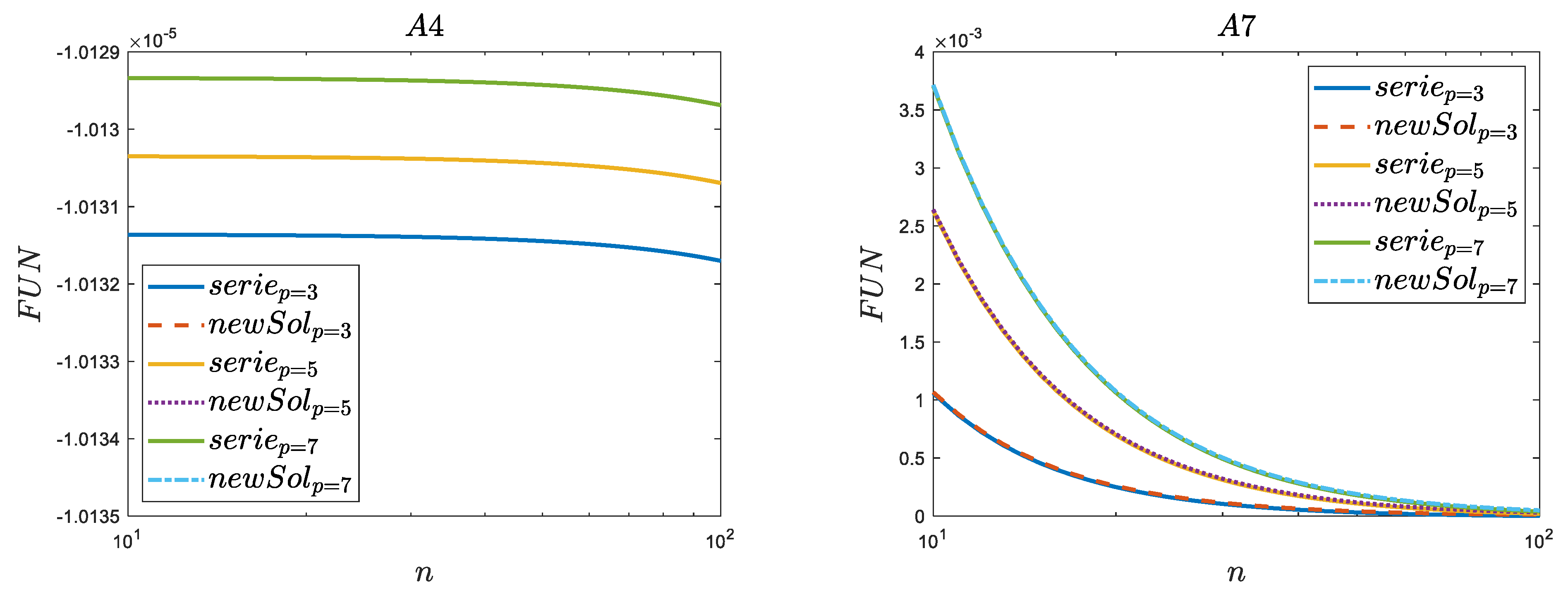
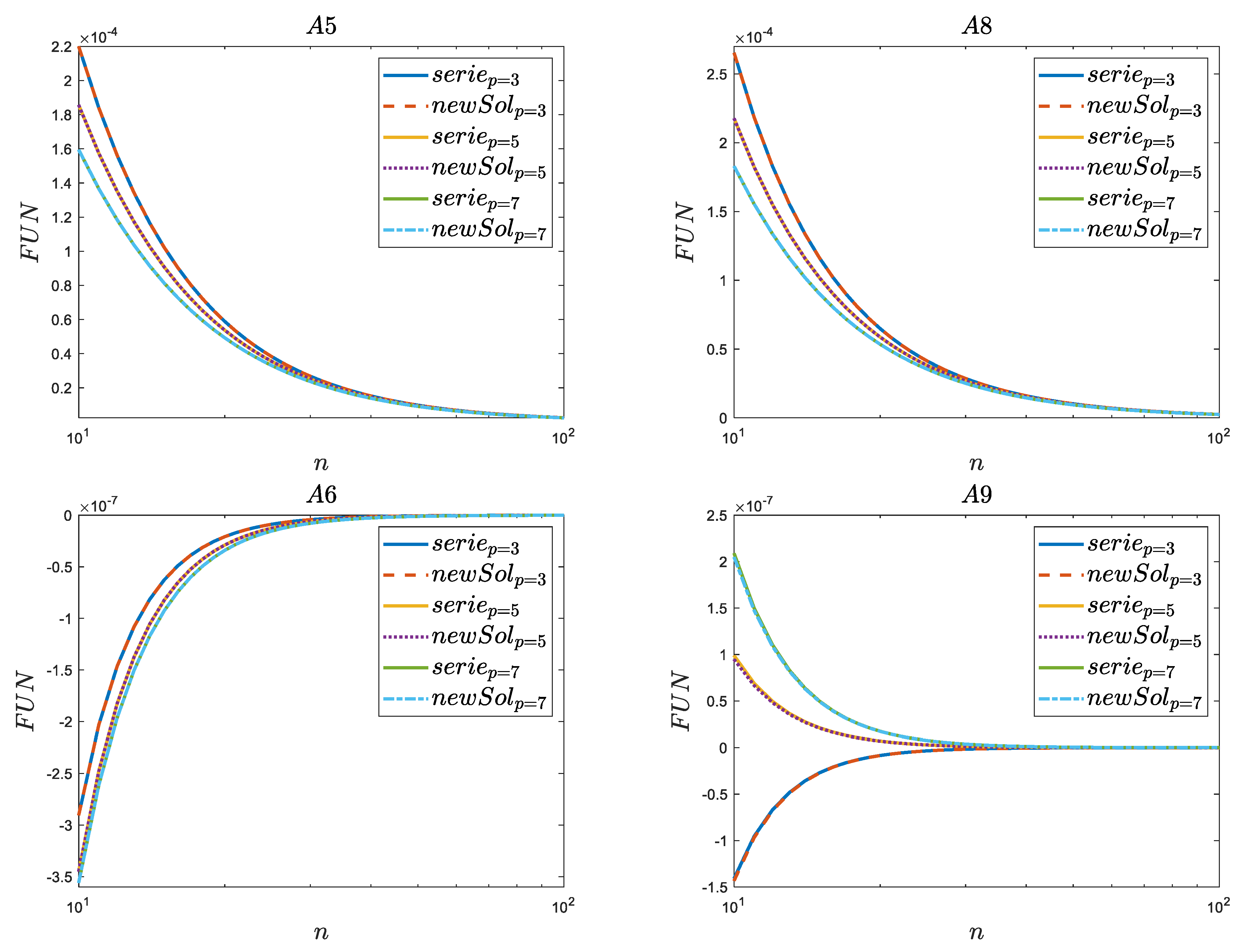
3.1. Analysis of Corrected Afanasiev Solutions (Difference of One Order)

The completed simulation tests in which the improved Afanasiev formulas (Equations (A4)–(A9)) were analyzed are shown in Figure 4. The tests were carried out for three assumed values of the orders of the Bessel function $p=1$, $p=3$ and $p=5$. The research for different p aimed to capture the trends in the obtained results.

From the analysis of the series described by Equation (A4) for $l=1,$ it follows that the solution to an infinite series of this type is always equal to zero, regardless of which Bessel root is subtracted ($j_{p+1,n}^2$) and what order of the Bessel function p was taken into account, the result always remains identical. This situation changes when the difference from the zeros of the Bessel function is raised to the second power, i.e., when $l=2$ Equation (A5). It can be seen here that when the first zero values of $j_{p+\mathrm{1,1}}^2$ are subtracted, the results obtained take maximum values, with the maximum value recorded for the lowest p values (case when $p=0$, not shown graphically). The larger the value of p, the lower the initial values of this analyzed function and the greater the flattening of the course toward the asymptotic value, i.e., 0. When $l=3$ in Equation (A6), it can be seen that this function starts with negative values and gradually increases with the subsequent subtraction of zeros (as n increases) until it reaches an asymptotic zero value (as in the previously analyzed case of Equation (A5)). This case also shows that for $l=3$, a few steps (n ≈ 10) are enough for this function to reach values that are close to asymptotic. The above means that significant results changes are visible only for low values of n, while higher values of n results are very similar.

An analysis of the solutions collected in the right column of Table A1 (Equations (A7)–(A9)), i.e., those in which the differences are in the denominator of the series, and the zeros of the Bessel function of one order lower ($j_{p-1,n}^2$) are subtracted, showing that the following:

-

When $l=1,$ the maximum values for $n=1$ are obtained at the lowest p value; in this case, $p=1$ (in the analysis it was not possible to assume a lower value, i.e., $p=0$, because then the zeros of the function $j_{-1,n}^2$ would be subtracted, and this is what we wanted to avoid). The obtained results show that for lower values of p, the dynamics of the decrease in the function value with increasing values of n were greater, as evidenced by the fact that the results for $n=2, 3, 4\dots$ were lower when the difference from the zeros of the higher orders of the Bessel function were taken into account;

-

Situations with changing dynamics were not noticed when $l=2$ and Equation (A8) were analyzed. Here, the shape of the function course and the values remained at a level very similar to those obtained from Equation (A5);

-

An interesting behavior was shown by the analysis of Equation (A9) obtained with power $l=3$. It can be seen from the graph that for $p=1,$ the values of this function for $n=2, 3, 4\dots$ were negative, while a similar behavior was not observed for larger values of $p\ge 3$ (values only positive). The zoom of Figure 4 for n ≥ 10 is presented in Appendix D.

To sum up, it should be noted that from all graphical comparisons presented (Figure 4), one can clearly see the complete perfect agreement of the proposed polynomial solution, which describes the infinite series based on these differences from the zeros of the Bessel function.

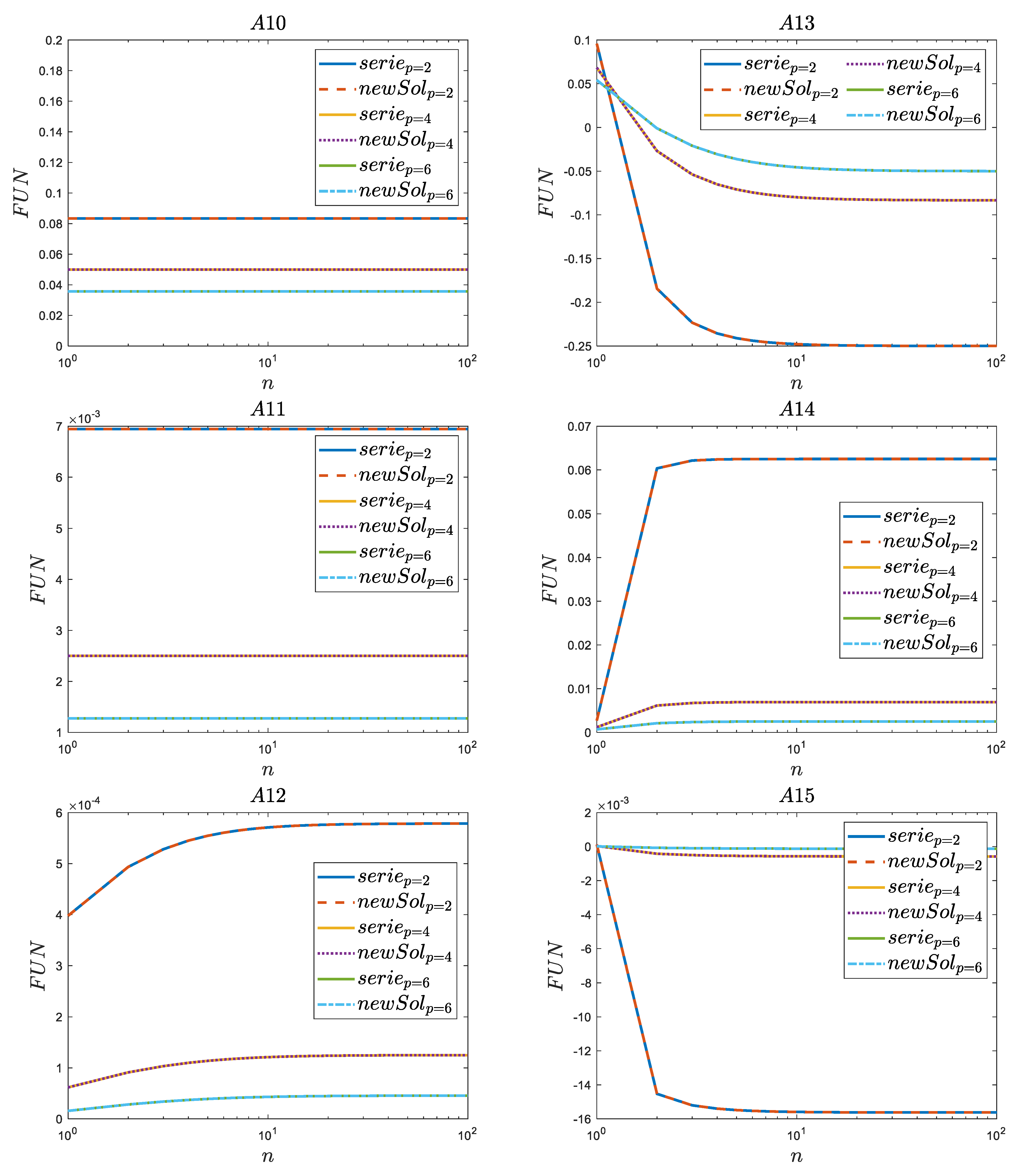
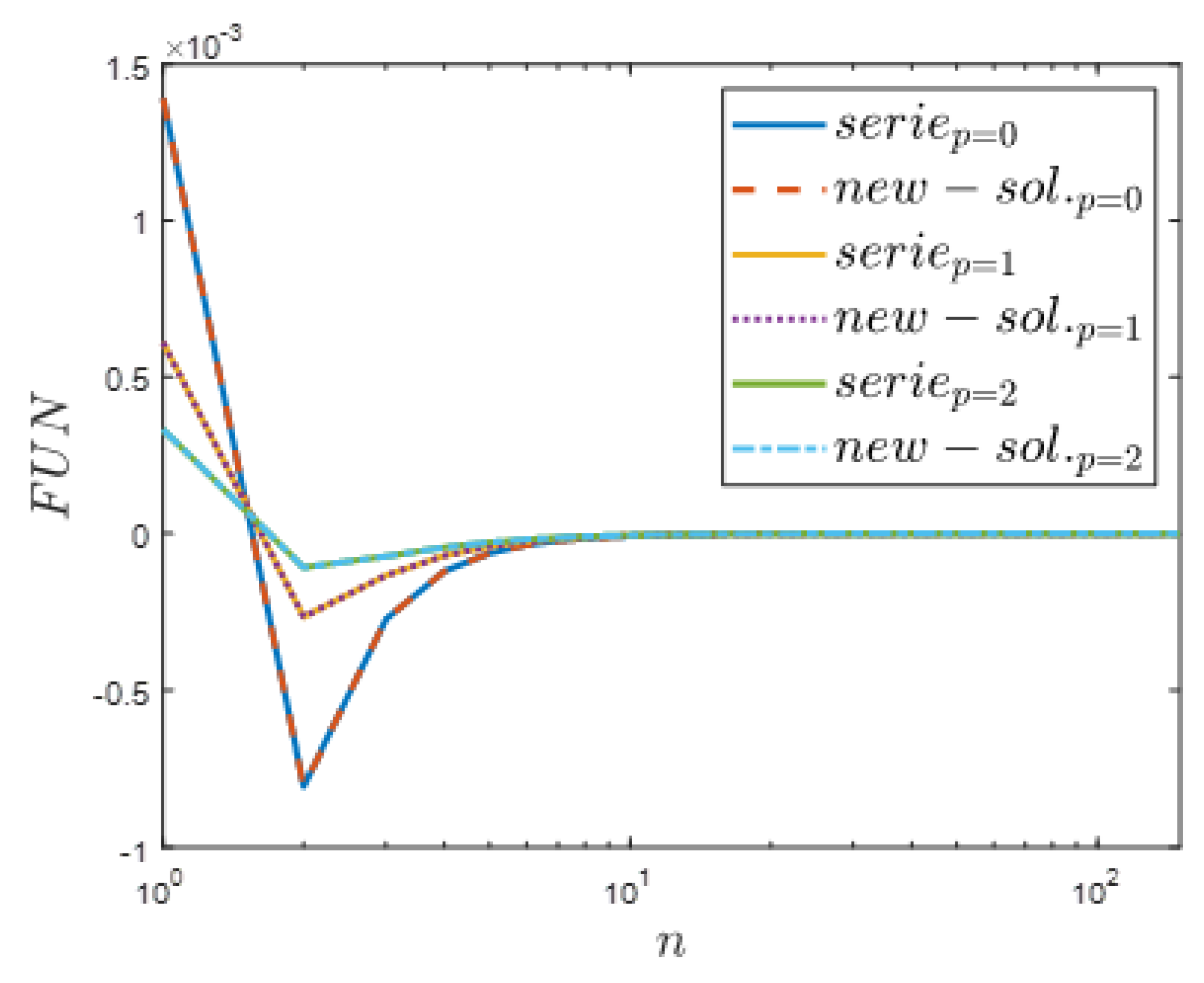
3.2. Analysis of New Solutions (Difference of Two Orders)

Figure 5 presents the selected simulation results. Again, the compatibility of the newly derived simplified polynomial formulas using the method proposed in this work with solutions calculated using infinite series is seen. The first to be analyzed are solutions ((A10), (A11) and (A12)), when the denominators of the series has a difference from such zeros $j_{p,k}^2-j_{p+2,n}^2$, and then the cases ((A13), (A14) and (A15)) are briefly discussed in which the difference in the denominator is as follows: $j_{p,k}^2-j_{p-2,n}^2$. Unlike the examples analyzed in Section 3.1, here, three cases of Bessel function orders $p=2$, $p=4$ and $p=6$ were analyzed. As before, the smallest value $p=2$ was chosen with the intention that in the formulas Equations (A13)–(A15) the problem with having to subtract the zeros of the Bessel function of negative orders was eliminated.

The results obtained from comparisons performed for the series defined by Equation (A10) indicate that the final result depends only on the order of the Bessel function p. There is no subtracted zero in the final formula; hence, it has no impact on the form of the course. The above affects the courses of these series, which are then straight lines. The larger the order of the function whose zero was considered, the smaller the results that are observed. Interestingly, when $l=2$ in the next series of Equation (A11), the situation is very similar. The results also did not depend on the subtracted zero and on the graph, and it was again possible to observe the constant course of these functions. The values of these functions obtained using Equation (A11) were definitely lower than in the case of Equation (A10). This was influenced by the derived polynomial form of this series, which, in this case, for $l=2$ was the square of the solution for $l=1$. When $l=3$, i.e., in the case of Equation (A12), a gradual increase in the results became visible as n increased. The reason for this increase was the appearance of the subtracted zero in the final simplified polynomial solution of Equation (A12).

The numerical results for $l=1$ were obtained using formula Equation (A13), showing that the larger the order of the Bessel function whose zeros were subtracted, the smaller the positive initial value (obtained for $n=1$). The values of all analyzed series when $n=2$ were assumed to take negative values. The final asymptotic value to which these infinite series tended as n approached infinity was also negative. The final asymptotic values had lower negative values as p increases. The results obtained for Equation (A14) showed that for $l=2$, the entire variability of the analyzed series almost ceased when n ≥ 4 for the subtracted zeros. The larger the p value, the more flattened the course was and the lower the positive asymptotic value. The plots obtained for $l=3$ from Equation (A15) are like a mirror image of those discussed just above when Equation (A14) was analyzed. With the difference here, apart from the negative sign, the results were characterized by significantly lower values. However, here too, the greatest variability of the curves was observed for the first $n=1, 2$ and 3 zeros.

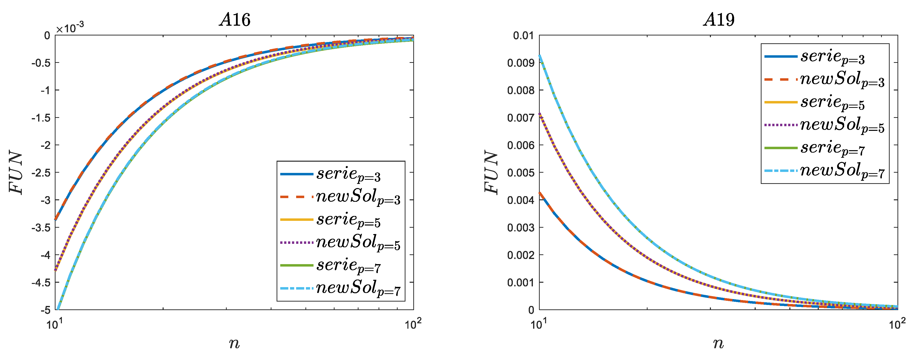
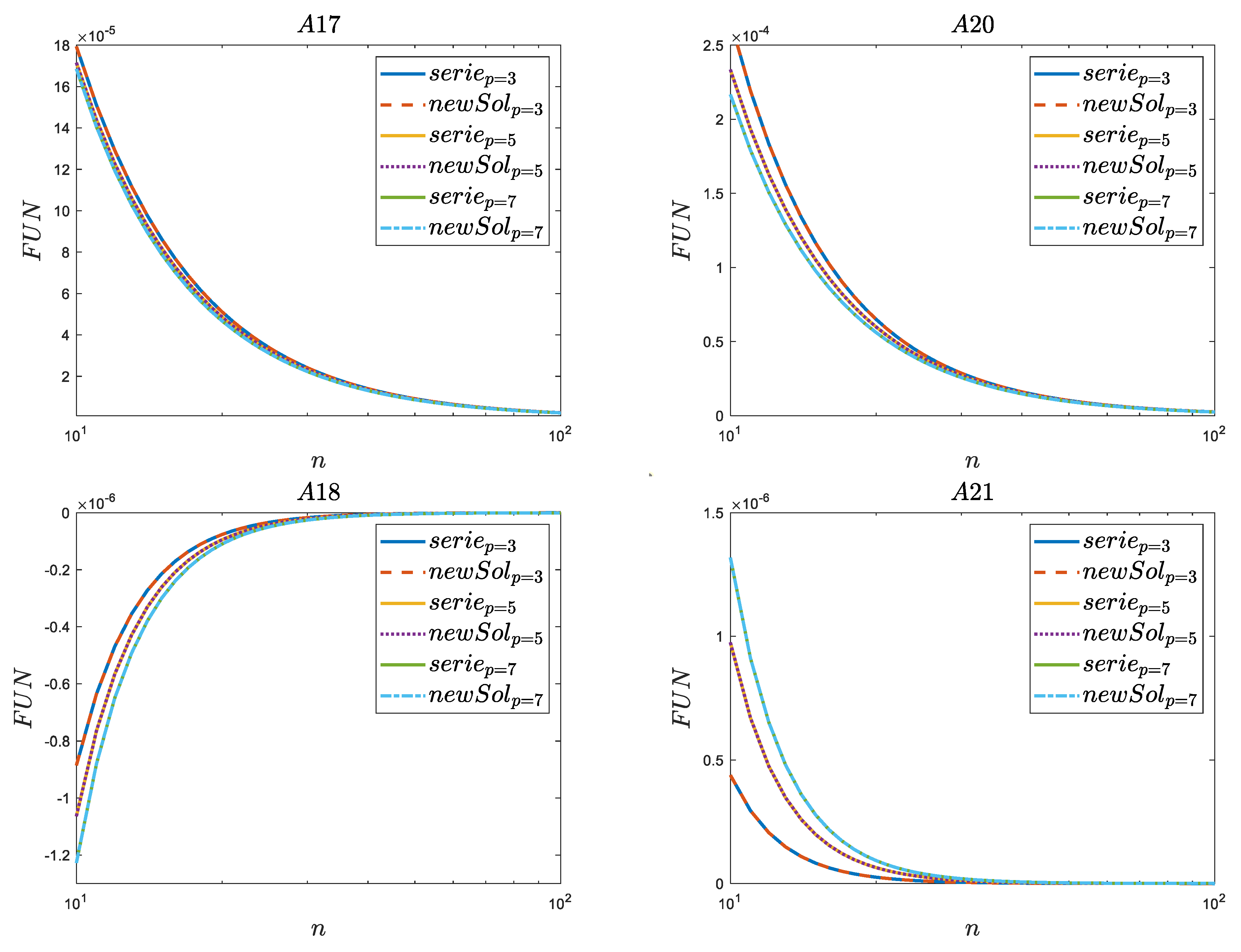
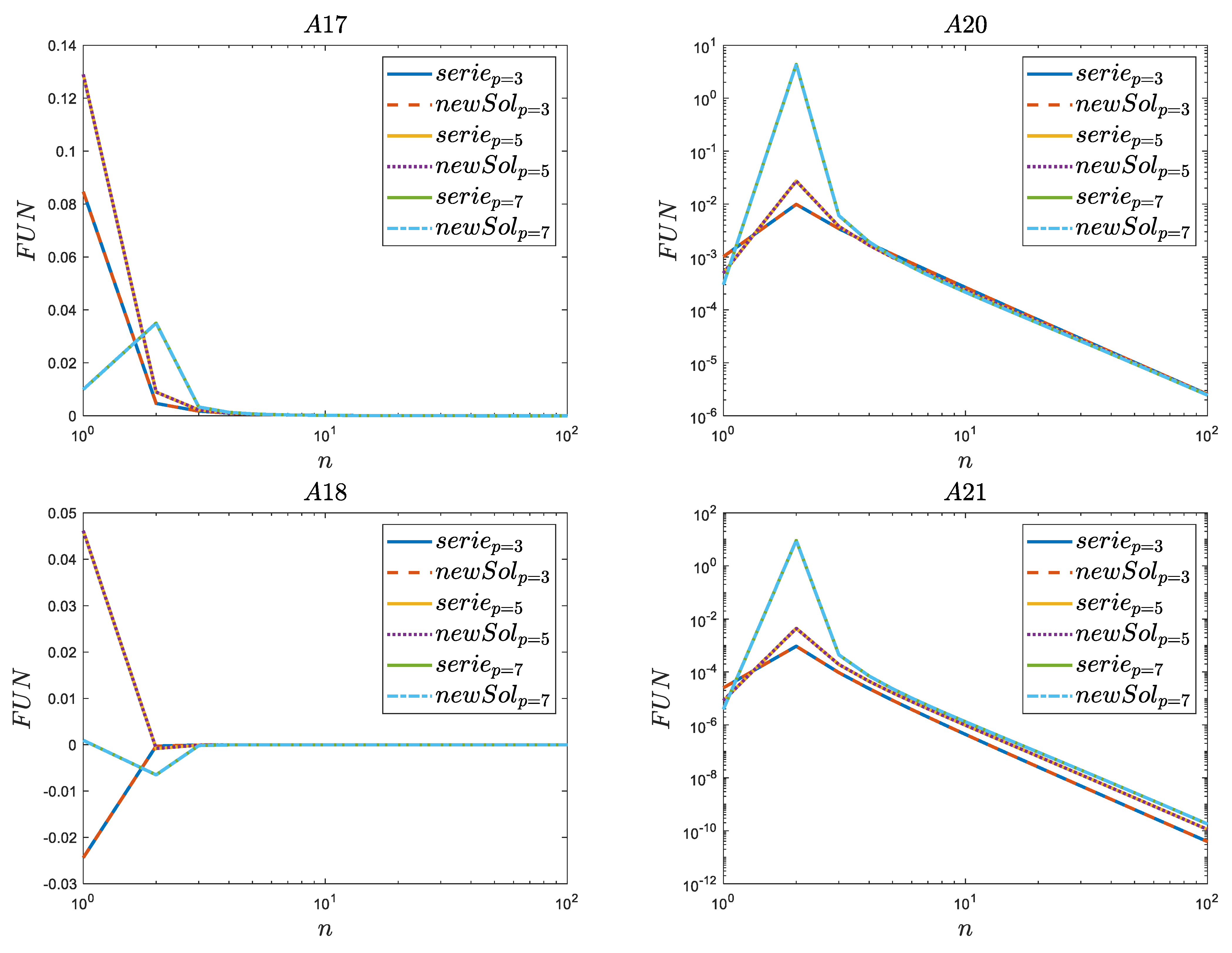
3.3. Analysis of New Solutions (Difference of Three Orders)

The last numerically analyzed results from this work (presented in Figure 6) concern series whose denominators had differences between the zeros of the Bessel function differing by three orders. To avoid subtracting zeros of the Bessel function of negative orders for comparisons, the lowest p value was set at $p=3$ (the next trends to observe were $p=5$ and $p=7$).

The obtained test results for Equations (A16)–(A18) were characterized by the fact that no clear (one-way) tendency was visible. In the case of $l=1$ in Equation (A16) it can be seen that the solution for $p=3$ had an increasing character as the value of n increased (with an initial negative value obtained for $n=1$), while in the case of $p=5$ and $p=7,$ it was clear that the initial values obtained for $n=1$ were positive and then there was a sharp drop to negative values. Thus, the tendency of these series became close to each other from $n=2$. An analysis of formula Equation (A17) showed that, this time, the initial tendency was similar for the series assuming $p=3$ and $p=5$, while the course at $p=7$ was characterized by a peak value obtained for $n=2$. Similarly, analyzing the results of $l=3$ obtained from the formula Equation (A18), there was no single trend visible because the initial value (for $n=1$) obtained at $p=3$ was negative, while for $p=5$ and $p=7$ these were positive initial values. Additionally, the absolute initial value was highest when $p=5$. The above indicates that with a difference of zeros by three orders in the denominators, we started to deal with complicated mathematical formulas that describe this series.

Interestingly, the graphical analysis of solutions for $l=1$ Equation (A19), $l=2$ Equation (A20) and $l=3$ Equation (A21) showed a similar behavior to the trend for functions in which $j_{p,k}^2-j_{p-3,n}^2$. Due to the fact that in each of the analyzed cases, Equations (A19)–(A21), the results had positive values, and exceptionally, these results could be presented on a logarithmic–logarithmic scale. This choice of scale was forced by the presence of a peak in the values of the series in these solutions, occurring in all cases for n = 2. The value of this peak in each of the tested series, i.e., for $l=1,2$ and 3, is greater than the $p$ value. The zoom of Figure 6 for n ≥ 10 is presented in Appendix D.

4. Practical Examples

4.1. Example I

During studies about wall shear stress occurring in pipe walls when an unsteady pipe flow takes place, an interesting convolution integral appears during the transformations needed to obtain the final time domain solution:

$$\frac{{8\nu v}_0\mu }{R^3}{\int }_0^t{\sum }_{i=1}^{\infty }{e}^{-\frac{\nu }{R^2}{{\eta }_i}^2\left(t-u\right)}{\sum }_{j=1}^{\infty }{e}^{-\frac{\nu }{R^2}{\xi }_j^{2}u}du$$

(43)

where ${\xi }_j$ is the root of the Bessel function of zero order $J_0\left({\xi }_j\right)=0$ and ${\eta }_j$ is the root of the Bessel function of the second order $J_2\left({\eta }_j\right)=0$. The above convolution defined by Equation (43) shows up as a result of the shear stress (in time domain) at the valve when a second possible analytical solution (Equation (28) from Zielke’s thesis [23]) is used for modelling the wall shear stress (nowadays, the commonly used solution is the one defined by Equation 35 in Zielke’s thesis [23]).

This Cauchy product of two infinite exponential generalized Dirichlet’s series Equation (43) has an analytical solution in the following form:

$$8\frac{v_0\mu }{R}{\sum }_{i=1}^{\infty }{\sum }_{j=1}^{\infty }\frac{e^{-\frac{\nu }{R^2}t{\xi }_j^2}-e^{-\frac{\nu }{R^2}{{\eta }_i}^{2}t}}{{{\eta }_i}^2-{\xi }_j^2}$$

(44)

The analytical solution discussed in this paper facilitates the simplification of the aforementioned double sum into more manageable single sums. The transformation is shown step by step below. First, let us write our solution in the form of two double series:

$$\begin{gathered} 8\frac{v_0\mu }{R}\left({\sum }_{j=1}^{\infty }{e}^{-\frac{\nu }{R^2}t{\xi }_j^2}{\sum }_{i=1}^{\infty }\frac{1}{{{\eta }_i}^2-{\xi }_j^2}-{\sum }_{i=1}^{\infty }{e}^{-\frac{\nu }{R^2}{{\eta }_i}^{2}t}{\sum }_{j=1}^{\infty }\frac{1}{{{\eta }_i}^2-{\xi }_j^2}\right)= \\ 8\frac{v_0\mu }{R}\left({\sum }_{j=1}^{\infty }{e}^{-\frac{\nu }{R^2}t{\xi }_j^2}{\sum }_{i=1}^{\infty }\frac{1}{{{\eta }_i}^2-{\xi }_j^2}+{\sum }_{i=1}^{\infty }{e}^{-\frac{\nu }{R^2}{{\eta }_i}^{2}t}{\sum }_{j=1}^{\infty }\frac{1}{{{{\xi }_j^2-\eta }_i}^2}\right) \end{gathered}$$

(45)

Compared with the solutions presented in Appendix A of this paper (A10 and A13), it can be seen that

$$\left\{\begin{array}{c}{\sum }_{i=1}^{\infty }\frac{1}{{{\eta }_i}^2-{\xi }_j^2}\equiv {\sum }_{\begin{array}{c}k=1\\ \end{array}}^{\infty }\frac{1}{j_{2,k}^2-j_{0,n}^2}=\frac{2}{j_{0,n}^2}-\frac{1}{4\left(2-1\right)} where: p=2\\ {\sum }_{j=1}^{\infty }\frac{1}{{{{\xi }_j^2-\eta }_i}^2}\equiv {\sum }_{\begin{array}{c}k=1\\ \end{array}}^{\infty }\frac{1}{j_{0,k}^2-j_{2,n}^2}=\frac{1}{4\left(1+0\right)} where: p=0\end{array}\right.$$

(46)

So,

$$\left\{\begin{array}{c}{\sum }_{i=1}^{\infty }\frac{1}{{{\eta }_i}^2-{\xi }_j^2}=\frac{2}{{\xi }_j^2}-\frac{1}{4} where: p=2\\ {\sum }_{j=1}^{\infty }\frac{1}{{{{\xi }_j^2-\eta }_i}^2}=\frac{1}{4} where: p=0\end{array}\right.$$

(47)

Thus, Equation (45) can be written with the help of Equation (47)

$$\begin{gathered} 8\frac{v_0\mu }{R}\left({\sum }_{j=1}^{\infty }{e}^{-\frac{\nu }{R^2}t{\xi }_j^2}\left(\frac{2}{{\xi }_j^2}-\frac{1}{4}\right)+\frac{1}{4}{\sum }_{i=1}^{\infty }{e}^{-\frac{\nu }{R^2}{{\eta }_i}^{2}t}\right)=8\frac{v_0\mu }{R}\left(2{\sum }_{j=1}^{\infty }\frac{e^{-\frac{\nu }{R^2}t{\xi }_j^2}}{{\xi }_j^2}- \\ \frac{1}{4}{\sum }_{j=1}^{\infty }{e}^{-\frac{\nu }{R^2}t{\xi }_j^2}+\frac{1}{4}{\sum }_{i=1}^{\infty }{e}^{-\frac{\nu }{R^2}{{\eta }_i}^{2}t}\right) \end{gathered}$$

(48)

The convolutional integral solution Equation (48) played a crucial role in demonstrating that the analytical solution for the unsteady wall shear stress at the downstream end valve section of a single pipe, induced by a rapid (instantaneous) valve closure, ultimately simplifies to

$${\tau }_{valve}=\frac{2v_0\mu }{R}{\sum }_{i=1}^{\infty }{e}^{-\frac{\nu }{R^2}{{\eta }_i}^{2}t}$$

(49)

A similar solution was recently derived [24] in a slightly simpler way.

4.2. Example II

The second example is also related to the fluid flow in pipes. Vogelpohl analyzed the accelerated flow in the pipe [25] by assuming a constant bulk velocity during the accelerating period. This led to the Voltera convolutional integral of the first kind that needed to be solved to find the pressure gradient time dependence. Using the Whitaker method [26], he was able to solve this problem. The coefficient of the exponential function of the pressure gradient solution was found from the roots of equations of the following type:

$${\sum }_{j=1}^{\infty }\frac{4}{x+{\xi }_j^2}=1 \Rightarrow {\sum }_{j=1}^{\infty }\frac{1}{x+{\xi }_j^2}=\frac{1}{4}$$

(50)

An analysis of this summation shows that these roots are only present for $x\le 0$. Vogelpohl found the first roots to be as follows: $x_1=0; x_2=-26.374; x_3=-70.849; x_4=-135.023; x_5=-218.922$. Vogelpohl did not notice that these roots (except for the minus sign) are the roots of the Bessel equation of the second order $J_2\left({\eta }_j\right)=0$.

All solutions were conducted with the minus sign; then, these solutions could be written to avoid the minus sign problem in the following form with positive values:

$${\sum }_{j=1}^{\infty }\frac{1}{{\xi }_j^2-x}=\frac{1}{4}$$

(51)

Inserting the zeros of the Bessel function $J_2\left({\eta }_j\right)=0$ for x made the equivalence of Equation (A10) evident:

$${\sum }_{\begin{array}{c}k=1\\ \end{array}}^{\infty }\frac{1}{j_{p,k}^2-j_{p+2,n}^2}=\frac{1}{4\left(1+p\right)}$$

(52)

In the Vogelpohl case p = 0, the final solution of A10 was exactly the same as the one derived by Vogelpohl

$${\sum }_{\begin{array}{c}k=1\\ \end{array}}^{\infty }\frac{1}{j_{0,k}^2-j_{2,n}^2}=\frac{1}{4\left(1+0\right)}=\frac{1}{4}$$

(53)

The above-presented examples show that such functions (series based on zeros of Bessel functions) can be found and are useful in real physical problems. Other practical examples found in the references are related to the following: (a) the problem of finding the eigenfunctions and eigenvalues of the free Schrödinger equation inside this cylinder [10]; (b) relativistic quantum mechanics (identity for the static polarizability) where transitions between the corresponding quantum states are related to the Thomas–Reiche–Kuhn sum rule [11].

Presented in this paper, the theory may contribute to the development of many practical issues found in applied science fields, such as (a) the electronics theory of passive n-parts (chapter 6 of [27]); (b) the analysis of time-domain responses of electrical networks and the synthesis of these circuits (amplifiers, etc.) with specified time domain characteristics [28,29,30]; (c) in communication circuits with an emitter current, the output voltages and average transconductance ratio of the modified Bessel function play the major role [31]; (d) analytical solutions for the transient and steady-state responses of linear time-invariant networks [32]; (e) finding the mean charge in graphene nanodots [33]; (f) dynamic analogy in the framework of a linear theory of viscoelasticity [34]; (g) electrical analogs of mechanical models [35]; (h) in mathematical fields, approximate expressions for Bessel functions zero, using a similar technique based on nonlinear equations for the zeros [36,37], the zeros of the equations arising in spectral problems [13,38], the identities between similar summation formulas [12], and important bounds [39,40] are found. The Calogero type series (some of which can be found in the upper part of Table A1) have been recently very useful in finding an inverse Laplace transform of a complicated frequency domain function [41].

5. Other Series and Their Possible Solutions

From the equation of the quotient of modified Bessel functions presented by Brühl in his recent paper [42], Equation (9),

$$\frac{I_0\left(x\right)}{I_2\left(x\right)}=1+\frac{8}{x^2}+\frac{2}{x}\frac{I_3\left(x\right)}{I_2\left(x\right)} \to \frac{I_0\left(\sqrt{x}\right)}{I_2\left(\sqrt{x}\right)}=1+\frac{8}{x}+\frac{2}{\sqrt{x}}\frac{I_3\left(\sqrt{x}\right)}{I_2\left(\sqrt{x}\right)}$$

(54)

And the formula derived by Brereton and Jiang [43], which was quoted in Urbanowicz et al.’s paper [44]:

$$\frac{I_0\left(\sqrt{x}\right)}{I_2\left(\sqrt{x}\right)}=1+\frac{8}{x}+4{\sum }_{i=1}^{\infty }\frac{1}{{\eta }_i^2+x}$$

(55)

${\eta }_i$—is the root of the Bessel function of the second order and $J_2\left({\eta }_i\right)=0.$ The following relationship for a ratio of modified Bessel functions can be found:

$$\frac{2}{\sqrt{x}}\frac{I_3\left(\sqrt{x}\right)}{I_2\left(\sqrt{x}\right)}=4{\sum }_{i=1}^{\infty }\frac{1}{{\eta }_i^2+x}$$

(56)

or

$${\sum }_{i=1}^{\infty }\frac{1}{{\eta }_i^2+x}=\frac{1}{2\sqrt{x}}\frac{I_3\left(\sqrt{x}\right)}{I_2\left(\sqrt{x}\right)}$$

(57)

The above formula can be applied to series based only on the zeros of the Bessel function, where $x$ is substituted with successive roots:

$${\sum }_{k=1}^{\infty }\frac{1}{{j_{p,k}^2+j}_{p,n}^2}=\frac{1}{2j_{p,n}}\frac{I_{p+1}\left(j_{p,n}\right)}{I_p\left(j_{p,n}\right)}$$

(58)

This analytical formula Equation (58) defines an infinite series of this type and is characterized by a summation in the denominator instead of a difference (as in the Calogero-Ahmed series). The validity of this function Equation (58) has been verified for selected $p\ge 0$, and it has been confirmed to operate accurately.

In Baricz et al.’s paper [45], an interesting equation is presented:

$${\sum }_{\begin{array}{c}k=1\\ k\ne n\end{array}}^{\infty }\frac{1}{{j_{p,k}^4-j}_{p,n}^4}=-\frac{1}{2j_{p,n}^2}\sum _{k=1}^{\infty }\frac{1}{{j_{p,k}^2+j}_{p,n}^2}+\frac{p+2}{4j_{p,n}^4}$$

(59)

This has been criticized by Anghel [46] because the infinite summation term (first on the r.h.s of Equation (59)) was still left in the equation: “…a proper evaluation … should not involve other sums of similar complexity, which is not the case for the paper under scrutiny”. However, the reader of Anghel’s paper [46] does not find a simplified final form of Equation (59) as Anghel introduces other infinite functions, namely $g\left(z\right)$ and its derivatives.

For this problem, when using Equation (58) in Equation (59), one obtains a final simplified explicit novel solution for this interesting type of series:

$$FUN={\sum }_{\begin{array}{c}k=1\\ k\ne n\end{array}}^{\infty }\frac{1}{{j_{p,k}^4-j}_{p,n}^4}=\frac{p+2}{4j_{p,n}^4}-\frac{1}{4j_{p,n}^3}\frac{I_{p+1}\left(j_{p,n}\right)}{I_p\left(j_{p,n}\right)}$$

(60)

The compatibility of the above Equation (60) was checked numerically for different values of $p=0,1,2$.

The received results presented in Figure 7 confirm the correctness of the proposed solution given by Equation (60). The figure also shows the progressive flattening of the results with the increase in the Bessel function $p$ order. For an additional example of the presented general summation formula defining the ratio of the modified Bessel function, please refer to Appendix E.

In this work, only examples related to fluid mechanics are presented, as this is the main research topic of the author of this work. The range of practical and theoretical issues whose mathematical description is based on functions of this type is very wide. An example is selected recent works [47,48,49,50,51,52,53], in which the theory presented in this manuscript can simplify the final forms of many presented formulas.

6. Conclusions

As noticed by many, including Watson [54], among them: “there are various classes of problems, connected with the zeros of Bessel functions…”. This paper discusses a series based only on the zeros of the Bessel function. It was noticed that the substitution of Lommel polynomials allowed the final result of the summation of a simple relationship based on the ratio of these polynomials to be simplified. These solutions have not been studied earlier in any branch of physics, mechanics or mathematics. New formulas extend the Rayleigh theory significantly [1]. This discussed series problem has not been studied in the old classics [54,55,56,57] and novel books [58,59].

The performed numerical analysis (with the help of programs written in Matlab) shows that the greatest differences in the variability of these solutions are noticed when the first and second zeros are subtracted (for n = 1 and 2). The conducted research also found that there are not always simple one-way variability trends when increasing the order of the Bessel function p and n. As can be seen from the table summarizing the new formulas, Table A1, the complexity relates to the values of the orders of the Bessel function, in which zeros are used for the calculations. The larger this difference, the more complex the form of the final polynomial.

By determining successive derivatives from the initial equation, it is possible to calculate more complex relationships obtained for larger values of the power of $l$ from the denominators of the analyzed functions. The problem of finding the final simplified general solution increases with each successive derivative. This is due to the lack of general formulas for determining the n-th derivatives of the function $f\left(z\right)=J_{p+1}\left(z\right)/J_p\left(z\right)$ or alternatively $g\left(z\right)=J_{p+1}\left(z\right)/\left(2z{J}_p\left(z\right)\right)$:

$$\frac{{\partial }^n}{{\partial z}^n}\left(\frac{J_{p+1}\left(z\right)}{J_p\left(z\right)}\right) \mathrm{and} \frac{{\partial }^n}{{\partial z}^n}\left(\frac{1}{2z}\frac{J_{p+1}\left(z\right)}{J_p\left(z\right)}\right)$$

(61)

The calculations realized in this paper show that the derivative of a function similar to the above one can always be written as a function depending on the original formula. The following solutions were obtained in this work:

$$\left\{\begin{array}{c}{h\left(z\right)}^{\prime }=A\left(p,z\right){h\left(z\right)}^2+B\left(p,z\right)h\left(z\right)+C\left(p,z\right)\\ {h\left(z\right)}^{″}=D\left(p,z\right){h\left(z\right)}^3+E\left(p,z\right){h\left(z\right)}^2+F\left(p,z\right)h\left(z\right)+G\left(p,z\right)\\ etc.\end{array}\right.$$

(62)

The obtained result implies that subsequent derivatives of the initial function can similarly be determined. Discovering similar formulas for the successive derivatives can contribute to the further simplification of the proposed solutions. In summary, future exploration of this topic should emphasize defining a specific rational function to characterize the following emerging coefficients: $A\left(p,z\right)$, $B\left(p,z\right)$, …, $F\left(p,z\right)$, $G\left(p,z\right)$, …

References

1. Rayleigh, L. Note on the numerical calculation of the roots of fluctuating functions. Proc. Lond. Math. Soc. 1873, 1–5, 119–124. [Google Scholar] [CrossRef]
2. Sneddon, I.N. On some infinite series involving the zeros of Bessel of the first kind. Proc. Glasg. Math. Assoc. 1960, 4, 144–156. [Google Scholar] [CrossRef]
3. Meiman, N.N. On recurrence formulas for power sums of zeros of Bessel functions. Dokl. Akad. Nauk SSSR 1956, 108, 190–193. [Google Scholar]
4. Kishore, N. The Rayleigh function. Proc. Am. Math. Soc. 1963, 14, 527–533. [Google Scholar] [CrossRef]
5. Elizalde, E.; Leseduarte, S.; Romeo, A. Sum rules for zeros of Bessel functions and an application to spherical Aharonov-Bohm quantum bags. J. Phys. A Math. Gen. 1993, 26, 2409–2419. [Google Scholar] [CrossRef]
6. Calogero, F. On the zeros of Bessel functions. Lett. Al Nuovo C. (1971–1985) 1977, 20, 254–256. [Google Scholar] [CrossRef]
7. Calogero, F. On the zeros of Bessel functions—II. Lett. Al Nuovo C. (1971–1985) 1977, 20, 476–478. [Google Scholar] [CrossRef]
8. Ahmed, S.; Calogero, F. On the zeros of Bessel functions—IV. Lett. Al Nuovo C. (1971–1985) 1978, 21, 531–534. [Google Scholar] [CrossRef]
9. Urbanowicz, K.; Stosiak, M.; Bergant, A. On the generalization of Calogero-Ahmed summation formulas. J. Phys. Conf. Ser. 2022, 2367, 012026. [Google Scholar] [CrossRef]
10. Afanasiev, G.N. Closed expressions for some useful integrals involving Legendre functions and sum rules for zeroes of Bessel functions. J. Comput. Phys. 1989, 85, 245–252. [Google Scholar] [CrossRef]
11. Pedersen, T.G. Sum rules for zeros and intersections of Bessel functions from quantum mechanical perturbation theory. Phys. Lett. A 2018, 382, 1837–1841. [Google Scholar] [CrossRef]
12. Ciaurri, Ó.; Durán, A.J.; Pérez, M.; Varona, J.L. Bernoulli–Dunkl and Apostol–Euler–Dunkl polynomials with applications to series involving zeros of Bessel functions. J. Approx. Theory 2018, 235, 20–45. [Google Scholar] [CrossRef]
13. Grebenkov, D.S. A physicist’s guide to explicit summation formulas involving zeroes of Bessel functions and related spectral sums. Rev. Math. Phys. 2021, 33, 2130002. [Google Scholar] [CrossRef]
14. VanSant, J.H. Conduction Heat Transfer Solutions; Report No.: UCRL-52863; Lawrence Livemore National Laboratory, California University: Livermore, CA, USA, 1980. [Google Scholar]
15. Han, J.C.; Wright, L.M. Analytical Heat Transfer, 2nd ed.; CRC Press: Boca Raton, FL, USA, 2022. [Google Scholar]
16. Irvan, I.; Zahedi, Z.; Agus, A.; Suparni, S.; Amin, H. Simplified Formulas for Some Bessel Functions and their Applications in Extended Surface Heat Transfer. BAREKENG J. Ilmu Mat. Dan Terap. 2022, 16, 507–514. [Google Scholar] [CrossRef]
17. Kung, K.Y.; Gong, M.F.; Srivastava, H.M.; Lin, S.D. Analytic Transient Solutions of a Cylindrical Heat Equation. Filomat 2021, 35, 2617–2628. [Google Scholar] [CrossRef]
18. Zare, M.; Sadeghi, S.; Xiong, Q. Analytical and numerical solutions for transient heat conduction in an infinite geometry with heat source subjected to heterogeneous boundary conditions of the third kind. J. Therm. Anal. Calorim. 2021, 143, 725–736. [Google Scholar] [CrossRef]
19. Magnus, W.; Oberhettinger, F.; Soni, R.P. Formulas and Theorems for the Special Functions of Mathematical Physics, 3rd ed.; Springer: Berlin, Germany, 1966. [Google Scholar] [CrossRef]
20. Lommel, E. Studien über die Bessel’schen Functionen; Druck und Verlag von B.G. Teubner: Leipzig, Germany, 1868. [Google Scholar]
21. Lommel, E. Zur Theorie der Bessel’schen Functionen. Math. Ann. 1871, 4, 103–116. [Google Scholar] [CrossRef]
22. Dickinson, D. On Lommel and Bessel polynomials. Proc. Amer. Math. Soc. 1954, 5, 946–956. [Google Scholar] [CrossRef]
23. Zielke, W. Frequency-Dependent Friction in Transient Pipe Flow. Ph.D. Thesis, University of Michigan, Ann Arbor, MI, USA, 1966. [Google Scholar]
24. Urbanowicz, K.; Bergant, A.; Stosiak, M.; Karpenko, M.; Bogdevičius, M. Developments in analytical wall shear stress modelling for water hammer phenomena. J. Sound Vib. 2023, 562, 117848. [Google Scholar] [CrossRef]
25. Vogelpohl, G. 15. Uber die Ermittlung der Rohreinlaufstromung aus den Navier-Stokesschen Gleichungen. ZAMM—J. Appl. Math. Mech. Z. Angew. Math. Mech. 1933, 13, 446–447. [Google Scholar] [CrossRef]
26. Whittaker, E.T. On the numerical solution of integral-equations. Proc. R. Soc. Lond. A 1918, 94, 367–383. [Google Scholar] [CrossRef]
27. Youla, D.C. Theory and Synthesis of Linear Passive Time-Invariant Networks; Cambridge University Press: Cambridge, UK, 2015. [Google Scholar]
28. Filanovsky, I.M. Enhancing amplifiers/filters bandwidth by transfer function zeroes. In Proceedings of the 2015 IEEE International Symposium on Circuits and Systems (ISCAS), Lisbon, Portugal, 24–27 May 2015; pp. 141–144. [Google Scholar] [CrossRef]
29. Filanovsky, I.M. Design of wide-band amplifiers/filters using Lommel polynomials. In Proceedings of the 2015 IEEE International Symposium on Circuits and Systems (ISCAS), Lisbon, Portugal, 24–27 May 2015; pp. 2672–2675. [Google Scholar] [CrossRef]
30. Su, K.L. Time Domain Synthesis of Linear Networks; Prentice-Hall: Saddle River, NY, USA, 1971. [Google Scholar]
31. Clarke, K.K.; Hess, D.T. Communication Circuits: Analysis and Design; Addison-Wesley: New York, NY, USA, 1971. [Google Scholar]
32. Li, J.C. Analytical solutions for the transient and steady-state responses of linear time-invariant networks. Int. J. Electron. 1993, 74, 423–439. [Google Scholar] [CrossRef]
33. Beneventano, C.G.; Fialkovsky, I.V.; Santangelo, E.M. Zeros of combinations of Bessel functions and the mean charge of graphene nanodots. Theor. Math. Phys. 2016, 187, 497–510. [Google Scholar] [CrossRef]
34. Giusti, A.; Mainardi, F. A dynamic viscoelastic analogy for fluid-filled elastic tubes. Meccanica 2016, 51, 2321–2330. [Google Scholar] [CrossRef]
35. Giusti, A.; Mainardi, F. On infinite series concerning zeros of Bessel functions of the first kind. Eur. Phys. J. Plus 2016, 131, 206. [Google Scholar] [CrossRef]
36. Campos, R.G.; Calderón, M.L. Approximate Closed-Form Formulas for the Zeros of the Bessel Polynomials. Int. J. Math. Math. Sci. 2012, 2012, 873078. [Google Scholar] [CrossRef]
37. Kerimov, M.K. Studies on the Zeroes of Bessel Functions and Methods for Their Computation: IV. Inequalities, Estimates, Expansions, etc., for Zeros of Bessel Functions. Comput. Math. Math. Phys. 2018, 58, 1–37. [Google Scholar] [CrossRef]
38. Kostin, A.B.; Sherstyukov, V.B. Calculation of Rayleigh type sums for zeros of the equation arising in spectral problem. IOP Conf. Ser. J. Phys. Conf. Ser. 2017, 937, 012022. [Google Scholar] [CrossRef]
39. Ismail, M.E.H.; Muldoon, M.E. Bounds for the small real and purely imaginary zeros of Bessel and related functions. Methods Appl. Anal. 1995, 2, 1–21. [Google Scholar] [CrossRef]
40. Baricz, Á.; Szász, R. The radius of convexity of normalized Bessel functions of the first kind. Anal. Appl. 2014, 12, 485–509. [Google Scholar] [CrossRef]
41. Urbanowicz, K.; Bergant, A.; Grzejda, R.; Stosiak, M. About Inverse Laplace Transform of a Dynamic Viscosity Function. Materials 2022, 15, 4364. [Google Scholar] [CrossRef]
42. Brühl, M. Analytical Solution for Laminar Water Hammer with Frequency-Dependent Friction. ASME J. Fluids Eng. 2022, 144, 111302. [Google Scholar] [CrossRef]
43. Brereton, G.J.; Jiang, Y. Exact solutions for some fully developed laminar pipe flows undergoing arbitrary unsteadiness. Phys. Fluids 2005, 17, 118104. [Google Scholar] [CrossRef]
44. Urbanowicz, K.; Haixiao, J.; Bergant, A.; Stosiak, M.; Lubecki, M. Progress in Analytical Modeling of Water Hammer. J. Fluids Eng. 2023, 145, 081203. [Google Scholar] [CrossRef]
45. Baricz, A.; Masirevic, D.J.; Pogany, T.K.; Szasz, R. On an identity for zeros of Bessel functions. J. Math. Anal. Appl. 2015, 422, 27–36. [Google Scholar] [CrossRef]
46. Anghel, N. On the paper “On an identity for the zeros of Bessel functions” by Baricz et al. J. Math. Anal. Appl. 2018, 468, 359–363. [Google Scholar] [CrossRef]
47. Fadel, M.; Raza, N.; Du, W.-S. Characterizing q-Bessel Functions of the First Kind with Their New Summation and Integral Representations. Mathematics 2023, 11, 3831. [Google Scholar] [CrossRef]
48. Huo, X.; Yang, W.; Jin, F.; Ben, S.; Song, X. Application of the Generalized Bessel Function to Two-Color Phase-of-the-Phase Spectroscopy. Mathematics 2022, 10, 4642. [Google Scholar] [CrossRef]
49. Usman, T.; Khan, N.; Martínez, F. Analysis of Generalized Bessel–Maitland Function and Its Properties. Axioms 2023, 12, 356. [Google Scholar] [CrossRef]
50. Li, A.; Qin, H. Fast Calculation of the Derivatives of Bessel Functions with Respect to the Parameter and Applications. Symmetry 2023, 15, 64. [Google Scholar] [CrossRef]
51. Zhu, L. New Bounds for the Modified Bessel Function of the First Kind and Toader-Qi Mean. Mathematics 2021, 9, 2867. [Google Scholar] [CrossRef]
52. Abramochkin, E.G.; Kotlyar, V.V.; Kovalev, A.A. Double and Square Bessel–Gaussian Beams. Micromachines 2023, 14, 1029. [Google Scholar] [CrossRef] [PubMed]
53. Dattoli, G.; Di Palma, E.; Licciardi, S.; Sabia, E. From Circular to Bessel Functions: A Transition through the Umbral Method. Fractal Fract. 2017, 1, 9. [Google Scholar] [CrossRef]
54. Watson, G.N. A Treatise on the Theory of Bessel Functions, 2nd ed.; Cambridge University Press: Cambridge, UK, 1966. [Google Scholar]
55. Gray, A.; Mathews, G.B. A Treatise on Bessel Functions and Their Applications to Physics, 2nd ed.; Macmillan and Company, Limited: London, UK, 1952. [Google Scholar]
56. Bowman, F. Introduction to Bessel Functions, 1st ed.; Dover Publications: New York, NY, USA, 1958. [Google Scholar]
57. McLachlan, N.W. Bessel Functions for Engineers, 2nd ed.; Clarendon Press: Oxford, UK, 1955. [Google Scholar]
58. Korenev, B.G. Bessel Functions and Their Applications, 1st ed.; CRC Press LLC: Boca Raton, FL, USA, 2002. [Google Scholar]
59. Baricz, A.; Masirevic, D.J.; Pogany, T.K. Series of Bessel and Kummer-Type Functions; Lecture Notes in Mathematics; Springer International Publishing AG: Cham, Switzerland, 2017; Volume 2207. [Google Scholar] [CrossRef]
Figure 1. Comparison of selected standard Bessel functions of the few first orders (p = 0, 1, 2, 3).
Applsci 13 12932 g001
Figure 2. Comparison of selected ratios of Bessel functions.
Applsci 13 12932 g002
Figure 3. Comparison of selected ratios of Bessel functions.
Applsci 13 12932 g003
Figure 4. Comparison of selected results of Afanasiev series (serie) with the new polynomial solution (newSol)—difference of one order.
Applsci 13 12932 g004
Figure 5. Comparison of selected and newly derived series (serie) with the new polynomial solution (newSol)—difference of two orders.
Applsci 13 12932 g005
Figure 6. Comparison of selected newly derived series (serie) with the new polynomial solution (newSol)—difference of three orders.
Applsci 13 12932 g006aApplsci 13 12932 g006b
Figure 7. Comparison of simplified final summation formula (for p = 0, 1 and 2).
Applsci 13 12932 g007
Disclaimer/Publisher’s Note: The statements, opinions and data contained in all publications are solely those of the individual author(s) and contributor(s) and not of MDPI and/or the editor(s). MDPI and/or the editor(s) disclaim responsibility for any injury to people or property resulting from any ideas, methods, instructions or products referred to in the content.