An Intelligent Detection System for Surface Shape Error of Shaft Workpieces Based on Multi-Sensor Combination

Abstract

As the main components of mechanical products and important transmission components of mechanical motion, shaft workpieces (SW) need to undergo high-speed motion while also withstanding high torque motion, which has high processing requirements. At the same time, the processing quality of the workpieces determines the success of the entire processing process, and the quality-inspection methods and the accuracy of the technology directly affect the evaluation of the product. This paper designs an intelligent detection system for the surface shape error (SSE) of SW that combines multiple sensors. Based on the principle of sensor use and specific experimental status, the overall scheme of the detection system is designed, followed by research on the spatial positioning algorithm and surface measurement algorithm of the workpiece to be tested. We then compensate and correct the errors with the algorithm. The effectiveness of the system is verified by measuring the surface size of the workpiece. Finally, the radial circular runout error is taken as an example to verify the detection system. The results show that the measurement error is less than 5%, and the accuracy of the system is high.

1. Introduction

The large-scale production of the machinery manufacturing industry creates higher requirements for its quality inspection [1,2,3]. As an important factor in ensuring the quality of products and a bottleneck factor to limit the further expansion of production [4], how to detect the processing quality of products more efficiently and conveniently has become an urgent problem [5]. Surface shape error (SSE) is an important indicator of mechanical product quality [6], and currently, the Coordinate Measuring Machine (CMM) is widely used [7]. The relative shape of products is obtained by point contact measurement and sliding contact measurement, and the position information of products is traced back in the established three-dimensional coordinate system so as to realize the detection of the size and shape information of products, with high measurement accuracy [8]. However, CMM is more suitable for multi-element detection than single-element detection because of its high cost and long detection time. Therefore, there is still a certain distance in the application of rapid detection in parts processing.

Commonly used detection equipment is divided into contact and non-contact types. Zhao et al. [9] used a CMM to measure the symmetry error of the double bond groove in the hub hole. The contact measurement has high monitoring accuracy and is convenient to use, but it also has the defect of easily scratching the surface of the workpiece [10,11]. Leo et al. [12] measured the appearance and straightness of the rod through the camera array of a non-telecentric optical system. Non-contact measurement is fast and efficient, but it is affected by the environment, and it is difficult to guarantee the measurement accuracy [13].

As one of the typical parts of machines, shaft workpieces (SW) are often used to support transmission parts such as gears, cams, and pulleys [14,15,16]. When working, the rotational speed is relatively high, so it is generally necessary to bear a large load. The high-quality requirements for SW are the basic guarantee for the stability and safety of mechanical operation [17,18]. In this paper, SW are taken as the research object, and a set of efficient, accurate, and automatic detection systems is established by combining the contact sensor and non-contact sensor. The axis of the SW is measured by six grating displacement sensors. The surface shape is then measured with a line laser sensor. The method proposed in this paper combines the characteristics of contact and non-contact sensors with high accuracy and efficiency. This is demonstrated by taking the radial circular runout as an example.

2. Surface Shape Measurement Principle

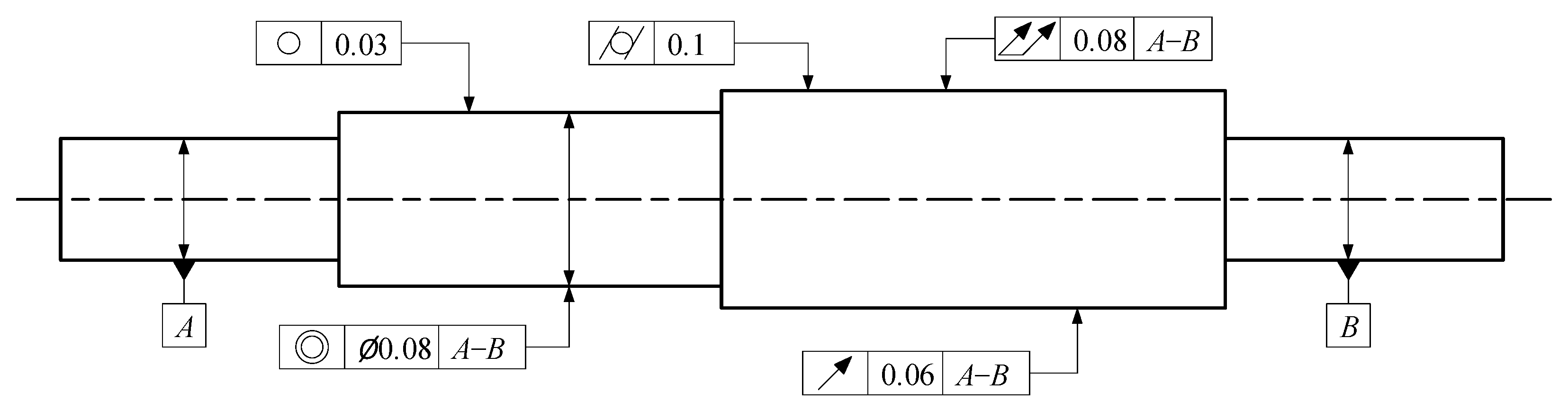
2.1. Measurement Elements for SSE of SW

The measurement elements of SW have a certain specificity. As shown in Figure 1, the SSE of the SW mainly includes roundness, cylindricity, coaxiality, radial circular runout, and radial full runout [19]. Among them, in the measurement of SW radial circular runout tolerance, the benchmark for the two ends of the journal formed by the common axis (A–B) is 0.06 mm. In the measurement of SW radial full runout tolerance, the benchmark for the two ends of the journal to determine the common axis (A–B) is 0.08 mm. The coaxiality tolerance is 0.08 mm. Roundness and cylindricity tolerances are 0.03 mm and 0.1 mm, respectively.

2.2. Detection Principle

2.2.1. Characteristics of the Sensor

The sensors selected in this paper include six contact grating probe sensors and a non-contact line laser sensor. The contact grating probe sensor is used to ensure the accuracy of the detection surface so as to ensure the accuracy of the spatial relative position of the workpiece. A non-contact line laser sensor is selected to realize non-contact measurement, which can avoid wear on the workpiece surface and can measure multiple points at one time so as to realize in situ detection and high measurement efficiency. All sensors can realize online measurement, which meets the development needs of modern enterprise digital manufacturing.

The grating probe measures the surface state and motion of the object through the optical principle. As a periodic and structured light-transmitting medium, the grating decomposes the light into several coherent beams and obtains the surface condition or motion state of the object by changing the phase difference between the coherent beams. In practical measurement applications, precision and accuracy are improved by adding tiny fiber gratings or wavelength-dependent structures. The grating probe has a wide range of application scenarios, often appearing in grating ruler to measure workpiece position and machine tool movement, robot precise positioning, and engineering measurement.

In this system, the surface parameters of the workpiece are detected by a line laser sensor. A line laser sensor can be viewed as a system of many point laser displacement sensors. As shown in Figure 2, the measurement principle of the point laser displacement sensor is laser triangulation. We provide a brief introduction below. The laser triangulation method calculates the spatial position, size, and shape of the measured object by measuring some parameters of the triangle. It uses the triangular relationship formed after the laser beam intersects with the measured object. The principle is that a laser beam is focused into a very small spot, which is irradiated on the surface of the measured object to form a reflected spot, and then the reflected light is received by the receiver and converted into an electrical signal for analysis and processing. By calculating the position of the reflected light spot on the detector, the distance between the center of the light spot to the detector, and the incident angle of the laser, the relevant information of the measured object can be calculated according to the triangulation principle. This method has the advantages of high measurement accuracy, high speed, and wide application range and is widely used in automatic production lines, logistics storage, and other fields.

In this paper, the normal incidence laser detection method is used. The distance between the height of the measured object and the reference plane changes the angle between the reflected light and the reference plane, and the angle of the incident light passing through the optical imaging equipment also changes, resulting in the displacement of the formed light spot. The displacement s is related to the height h of the measured object relative to the reference plane, so the height h can be represented by the displacement.

In Figure 2, ΔQBH and ΔQB₁G are similar, obtaining

$$\frac{\overline{BH}}{\overline{B_{1}G}}=\frac{\overline{QH}}{\overline{QG}}$$

(1)

According to plane geometry,

$$\left\{\begin{array}{c}\overline{BH}=h\sin (\theta )\\ \overline{B_{1}G}=s\sin (\phi )\\ \overline{QH}=l-\overline{AH}\\ \overline{AH}=h\cos (\theta )\\ \overline{QG}=g+\overline{A_{1}G}\\ \overline{A_{1}G}=s\cos (\phi )\end{array}\right.$$

(2)

This further obtains

$$\frac{h\sin \left(\theta \right)}{s\sin \left(\phi \right)}=\frac{l-h\cos \left(\theta \right)}{g+s\cos \left(\phi \right)}$$

(3)

Finally, the expression of h is obtained as

$$h=\frac{\left(l-f\right)\left(l-h\cos \theta \right)s\sin \phi }{\left[fl+\left(l-f\right)s\cos \phi \right]\sin \theta }$$

(4)

A line laser emits a light beam and traces its path. When the light is emitted to the surface of the object, it will be reflected and captured by the receiving device in the line laser sensor. According to the position of the received reflection point of each point, the relative spatial distance to each point on a laser can be calculated according to the laser triangulation method, which is expressed as the surface shape of the object on the display equipment.

The laser sensor has high precision and is convenient to use. When measuring SW, the best strategy is to make the detection line parallel to the axis so as to obtain the largest detection range. However, in practical experiments, it is found that when the laser is parallel to the axis, due to the above principle of laser detection—that is, the reflection effect of light, there are often problems of too large detection errors and noise, as shown in Figure 3a. The position of the red frame includes the wrong data, and all of the measurement data contain a lot of noise points. When the line laser sensor rotates at a certain angle, the detection effect is obviously improved, which can meet the measurement requirements in Figure 3b. Therefore, the system sets a certain angle between the straight line and the axis detected by the line laser sensor during measurement.

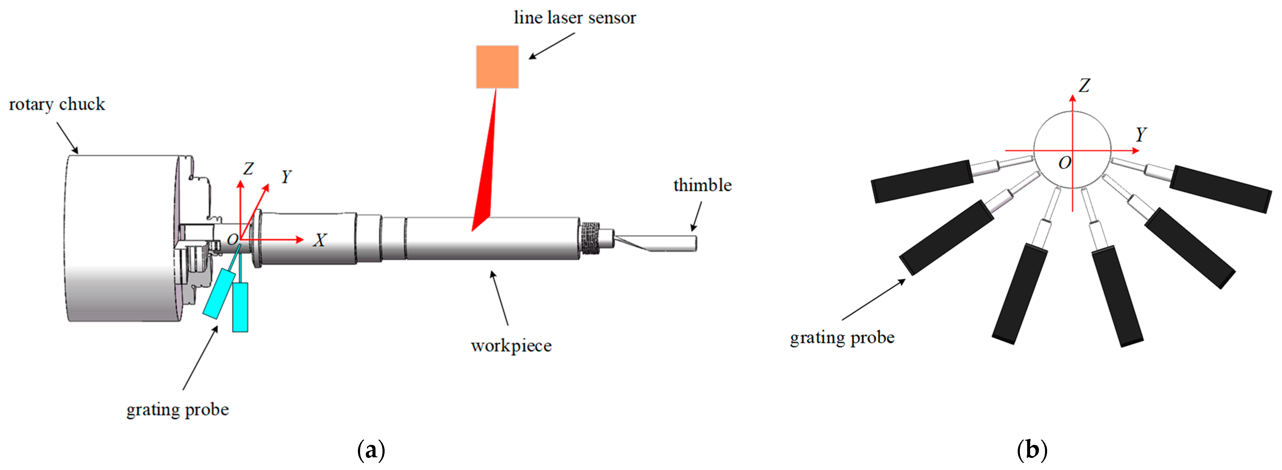
2.2.2. Overall Design of the Detection System

As a long rotary part, to determine its spatial position, we should determine the relative position of the axis in space and combine it with its prime line position. As shown in Figure 4, six grating probes are unevenly distributed on the lower half circle of a concentric circle in a vertical plane. The measuring plane, where the grating probes are located, is the Y–O–Z plane. The intersection point of the straight extension line, where the grating probes are located, is the space origin. And the cartesian left hand rule establishes the coordinate system O–X–Y–Z.

One end of the shaft usually features a cylindrical surface, assuming that the cylindrical surface intersects the Y–O–Z plane, as shown in the picture. According to the principle of spatial geometry, the intersection of the cylinder and plane is an ellipse, and the intersection of the axis and plane x = 0 is an ellipse. The essence of an ellipse is a conic. Through the probe, the multipoint coordinates on the Y–O–Z plane of the ellipse are obtained, and the ellipse is in the plane of x = 0 so as to obtain the spatial coordinate (0, y, z).

The general equation of an ellipse is

$$F(y,z)=a{y}^2+byz+c{z}^2+dy+ez+f=0$$

(5)

Among them a, b, c, d, e, and f are parameters, and there is a constraint: $b^2-4ac>0$.

Define the vector ${\mathit{A}}_{\mathit{x}}={[a,b,c,d,e,f]}^T$, $\mathit{X}=[y^2,yz,z^2,y,z,1]$. The problem of a curve fitting to a group of known points is expressed by the sum of squares of the minimum distance from point to the curve as

$$\underset{A}{\min }{\displaystyle \sum _{i=1}^n\mathit{F}{(y_i,z_i)}^2}=\underset{A}{\min }{\displaystyle \sum _{i=1}^n{({\mathit{X}}_i\cdot {\mathit{A}}_{\mathit{x}})}^2}$$

(6)

It is known that vector A_x multiplied by any coefficient is still the same equation; thus, the constraint condition can be transformed into $b^2-4ac=1$. The fitting problem in the ellipse data of the detection section can be expressed as

$$\underset{A}{\min }{‖\mathit{D}a‖}^2 \mathrm{Constraints}:{\mathit{A}}_{\mathit{x}}{}^T\mathit{C}{\mathit{A}}_{\mathit{x}}=1$$

(7)

Among them,

$$\mathit{D}=\left(\begin{array}{cccccc}{y}_1{}^2& y_1{z}_1& z_1{}^2& y_1& z_1& 1\\ ⋮& ⋮& ⋮& ⋮& ⋮& ⋮\\ y_i{}^2& y_i{z}_i& z_i{}^2& y_i& z_i& 1\\ ⋮& ⋮& ⋮& ⋮& ⋮& ⋮\\ y_n{}^2& y_n{z}_n& z_n{}^2& y_n& z_n& 1\end{array}\right),\mathit{C}=\left(\begin{array}{cccccc}0& 0& 2& 0& 0& 0\\ 0& -1& 0& 0& 0& 0\\ 2& 0& 0& 0& 0& 0\\ 0& 0& 0& 0& 0& 0\\ 0& 0& 0& 0& 0& 0\\ 0& 0& 0& 0& 0& 0\end{array}\right)$$

By using Lagrange multiplier and a series of simplified formulas, the elliptic curve equation can be solved through direct solution.

The center C_t$(x_0,y_0,z_0)$ of the ellipse can be obtained by using the ellipse equation with a known cross-section.

$$\left\{\begin{array}{l}{x}_0=0\\ y_0=\frac{be-2cd}{4ac-b^2}\\ z_0=\frac{bd-2ae}{4ac-b^2}\end{array}\right.$$

(8)

Determining the position of the spatial axis needs a point on the axis and the direction vector of the axis. It is known that the center of the ellipse is a point on the axis, so only the value of the direction vector is required next.

An ellipse is the intersection of a cylindrical surface and a plane. All points on the ellipse are on the cylindrical surface, and the distances from point $(x_i,y_i,z_i)$ to the axis on the ellipse are the same. The distance $S_i$ between the point $(x_i,y_i,z_i)$ and the straight line can be expressed as

$$S_i=\sqrt{\frac{\frac{1}{m^2}{\left(n\frac{\frac{z_i-z_0}{x_i-x_0}-\frac{p}{m}}{\frac{n}{m}-\frac{y_i-y_0}{x_i-x_0}}+p\right)}^2+{\left(\frac{\frac{z_i-z_0}{x_i-x_0}-\frac{p}{m}}{\frac{n}{m}-\frac{y_i-y_0}{x_i-x_0}}\right)}^2+1}{m^2+n^2+p^2}}$$

(9)

Therefore, the radius of the cylinder R is known as

$$\left\{\begin{array}{l}{S}_1=S_2\\ S_1=S_3\\ m^2+n^2+p^2=1\end{array}\right.$$

(10)

Arbitrary multiples of m, n, and p have no influence on the equation, and the formula $m^2+n^2+p^2=1$ ensures the uniqueness of the solution to the equation. Solve Equation (10) and determine the position of the spatial axis.

A point on its axis is measured using the instrumental method, and the direction vector of its axis is calculated to obtain the mathematical expression and spatial position of its axis. The point on the given axis is $(x_0,y_0,z_0)$, the direction vector is $(m,n,p)$, and the axis equation is

$$\frac{x-x_0}{m}=\frac{y-y_0}{n}=\frac{z-z_0}{p}$$

(11)

Then, the surface data of the shaft are obtained by the line laser sensor and the included angle α between the line laser displacement sensor and the X–O–Z plane. The conversion relationship between the detected value of the line laser sensor and the world coordinate system is as follows.

$$\left[\begin{array}{c}x\\ y\\ z\end{array}\right]=\left[\begin{array}{ccc}\cos \alpha & 0& 0\\ 0& \sin \alpha & 0\\ 0& 0& 1\end{array}\right]\left[\begin{array}{c}{x}_A\\ x_A\\ z_A\end{array}\right]$$

(12)

Among them, $x_A$, $z_A$ are detection values in the sensor coordinate system.

In order to facilitate analysis and calculation based on coordinate transformation, the surface data of the workpiece are converted into the surface data of the axis on the X axis, and the spatial position, translation, and rotation axis of the axis are known to make it coincide with the X axis. Because the axis is translated to coincide with the origin in advance, rotation will not affect the surface data of the circular axis.

Move point C_t to the origin O (0, 0, 0) of the world coordinate system in Figure 5, and the movement matrix is

$$\mathit{T}=\left[\begin{array}{cccc}1& 0& 0& -x_0\\ 0& 1& 0& -y_0\\ 0& 0& 1& -z_0\\ 0& 0& 0& 1\end{array}\right]$$

(13)

Then, rotate the straight line clockwise around the Z-axis rotation direction. The size of the rotation angle β and the rotation equation ${\mathit{T}}_1$ are as follows.

$$\beta =\arctan \frac{n}{m}$$

(14)

$${\mathit{T}}_1=\left[\begin{array}{cccc}\cos (-\beta )& -\sin (-\beta )& 0& 0\\ \sin (-\beta )& \cos (-\beta )& 0& 0\\ 0& 0& 1& 0\\ 0& 0& 0& 1\end{array}\right]$$

(15)

The rotation angle, angle size γ, and rotation equation ${\mathit{T}}_2$ around the Y-axis are as follows:

$$\gamma =\arctan \frac{p}{\sqrt{m^2+n^2}}$$

(16)

$${\mathit{T}}_2=\left[\begin{array}{cccc}\cos \gamma & 0& \sin \gamma & 0\\ 0& 1& 0& 0\\ -\sin \gamma & 0& \cos \gamma & 0\\ 0& 0& 0& 1\end{array}\right]$$

(17)

The conversion formula for converting the detected data into data with the axis on the X-axis is

$$\left[\begin{array}{c}{x}^{\prime }\\ y^{\prime }\\ z^{\prime }\\ 1\end{array}\right]=\mathit{T}{\mathit{T}}_1{\mathit{T}}_2\left[\begin{array}{c}x\\ y\\ z\\ 1\end{array}\right]$$

(18)

In the establishment of the surface measurement method, an important index is the determination of angle α.

Theoretically, angle α can be set at will, and a better angle needs to be determined in the actual experiment. Assuming that the amount of effective data obtained at that time of α = 0 is 0.8, when the dip angle reaches 45°, the effective data can basically be regarded as 1. But at the same time, the maximum data length that can be measured will be reduced, and at 45°, there are only 0.707 detection lengths. The weights of data accuracy and data amount are set to 7 and 3, respectively, and then an evaluation model is established as

$$\begin{array}{c}\min \left\{0.7\left(0.8+\frac{\alpha }{0.25\pi }\times 0.2\right)+0.3\left(\cos \alpha \right)\right\}\\ s.t 0<\alpha <0.25\pi \end{array}$$

(19)

The optimal solution is obtained for the above evaluation model, and the optimal value is 36.45°.

In the actual installation process, because the installation error may cause the actual value of the angle α to deviate from the set value, which will affect the experimental results, the standard cylinder is used to verify the actual included angle. Equation (20) can still be obtained from the detection data of the line laser sensor, and the distances from the detection points to the cylindrical axis are equal.

$$\left\{\begin{array}{l}{S}_1=S_2\\ S_2=S_3\end{array}\right.$$

(20)

Bring Equation (9) into Equation (20), and the rotation angle can be obtained via solution.

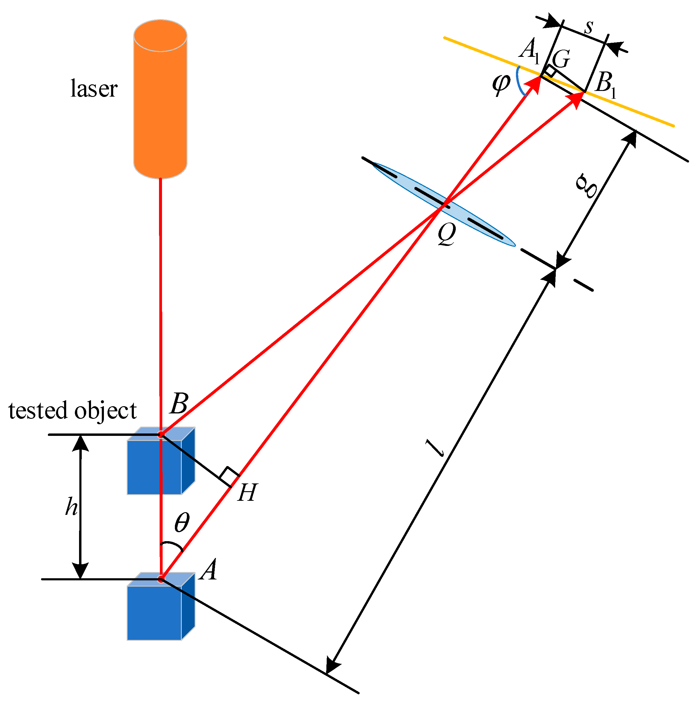
2.2.3. Radial Circular Runout Measurement Principle

As shown in Figure 6, the radial circular runout tolerance is evaluated using the maximum zone method. For the tolerance zone for any perpendicular to the base axis of the cross-section, the radius difference is equal to the tolerance value f, the center of the two concentric circles in the reference axis of the region bounded.

Taking radial circular runout as an example, this paper introduces the calculation using measured data. From the above, we can obtain the position of the spatial curve detected by the line laser sensor in the spatial rectangular coordinate system. The radial circular runout error solves the maximum difference between the spatial point and the center of the circle, which can be obtained by the distance from each measuring point to the center of the circle.

Knowing the measured data as $(x_i,y_i,z_i)$, solve the distance S from each data point to the axis. By calculating the rotating shaft piece, n points on a section after coordinate translation are obtained, and the distance from the i-th point on the j-th measurement to the axis is S_ji; thus, the difference of its maximum value is solved.

$$\left\{\begin{array}{c}{S}_{jmax}=\max (S_{ji}),i=\mathrm{1,2},\cdots ,n\\ S_{jmin}=\min (S_{ji}),i=\mathrm{1,2},\cdots ,n\end{array}\right.$$

(21)

where S_jmax is the maximum distance between the j-th measurement and the axis, and S_jmin is the maximum distance between the j-th measurement and the axis.

The radial circular runout S_Δj of the j-th measurement is

$$S_{\Delta j}=S_{jmax}-S_{jmin},j=\mathrm{1,2},\cdots ,m$$

(22)

The radial circular runout of the measured section is the maximum of m measurements:

$$S_{\Delta }=\mathit{max}(S_{\Delta j}),j=\mathrm{1,2},\cdots ,m$$

(23)

where S_Δ is the radial circular runout of the measured section.

2.3. Error Compensation and Calibration

2.3.1. Radial Installation Error

There will be radial installation errors when the sensor is installed, so the device is calibrated with a standard circular axis. As shown in Figure 7, the radius of the standard circle axis is r, and the detection value is 0 when the radius of the grating probe is $r_0$. We put the standard circular axis at the center of the circle measured by the grating sensor. Theoretically, the measured value of the grating probe should be $(r-r_0)$, and the actual detection value is d_ri, so the radial compensation required by the i-th grating probe is

$$\Delta x_{ri}=(r-r_0)-d_{ri}$$

(24)

where the compensation amount of the i-th probe is $\Delta x_{ri}$, the measured value of the i-th probe is d_ri, and the detection value $x_{rc}$ is

$$x_{rc}=\Delta x_{ri}+d_{ri}$$

(25)

2.3.2. Circumferential Installation Error

The grating sensor is also prone to circumferential errors in the installation process. There is a deviation angle $a_1$ between the mounting position and the predetermined position in Figure 8. The theoretical measured value of the grating sensor is $(r-r_0)$, and the actual measured value is $d_{ci}$

$$d_{ci}=d^{\prime }-(d^{\prime }+r_0)\cos a_1+\sqrt{r^2-{(d^{\prime }+r_0)}^2{\sin }^2{a}_1}$$

(26)

where d′ is the original length of the grating probe rod.

The deviation $\Delta x_{ci}$ between the actual value and the theoretical value is the error value that needs to be adjusted.

$$\Delta x_{ci}=(d^{\prime }+r_0)\cos a_1-\sqrt{r^2-{(d^{\prime }+r_0)}^2{\sin }^2{a}_1}-(d^{\prime }+r_0-r)$$

(27)

The compensated value is

$$x_c{}^{\prime }=\Delta x_{ci}+d_{ci}$$

(28)

2.3.3. Axial Installation Error

There is also an axial error between grating probes. The center lines of the probes are not in the same vertical plane, and the plane deviates from the theoretical position horizontally, as shown in Figure 9. The influence of axial deviation on the results is related to the inclination of the axis and needs to be evaluated.

An ellipse is measured, and the equation is $x^2+2xy+3y^2+4x+5y=6$. The coordinate of the center point is (−1.75, −0.25). Suppose that one of the six probes is offset in the horizontal direction but not found during the experimental installation; that is, the value of this position is $x+k$ recorded as the value of this position $x$, resulting in a 10% change in each detected value. Observe the influence of the center point position on the calculation results and take the distance between the obtained point and the theoretical value point as the reference index. The bigger the index, the greater the number of points. The result is shown in Figure 10a. The influence on the result when three consecutive measuring points are offset is shown in Figure 10b.

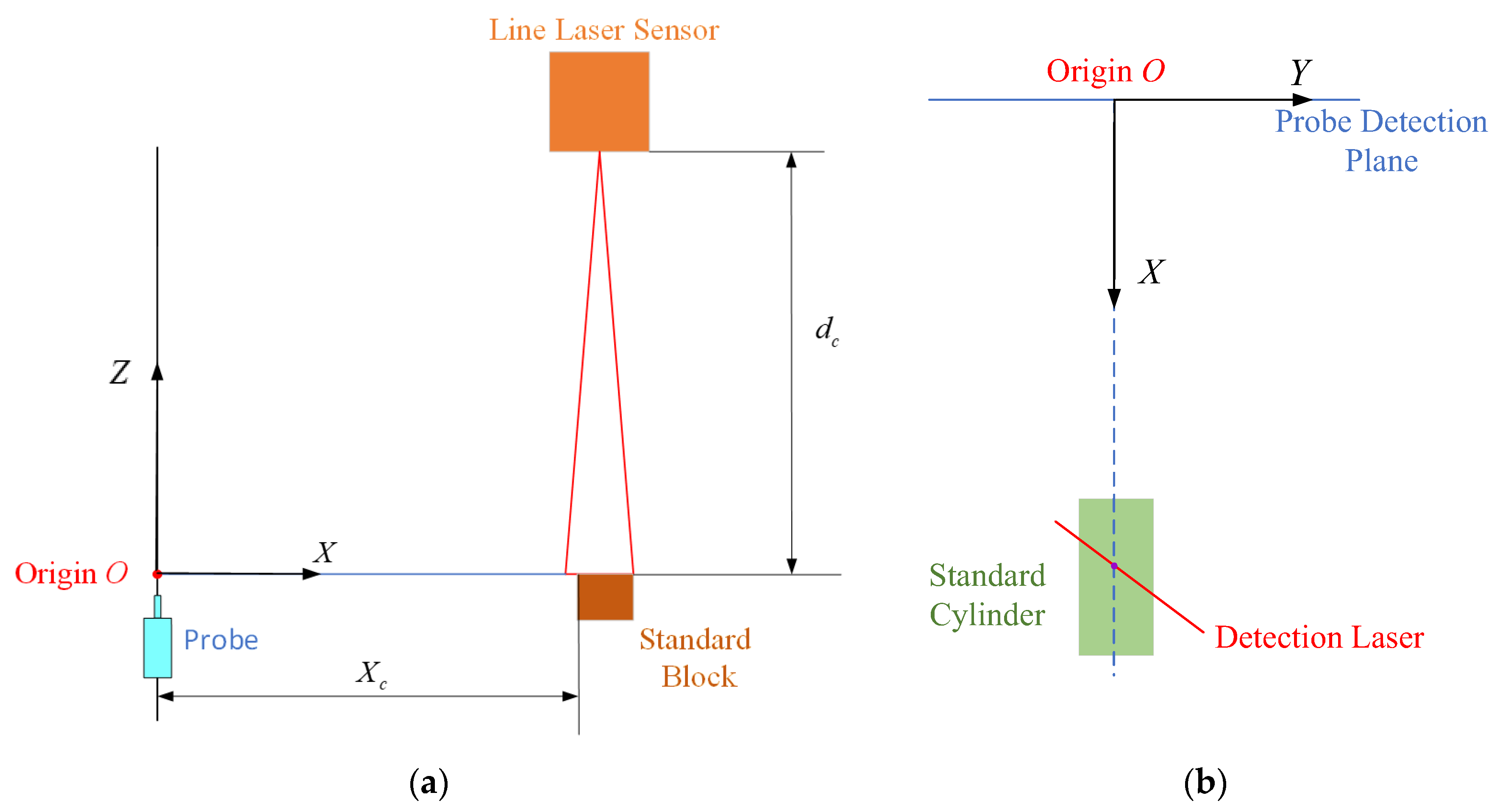
2.3.4. Calibration of the Detection System

As can be seen in Figure 9, when the sensor is axially offset, it will have a great impact on the selection of the center point, especially when the point near the center is displaced. Therefore, it needs to be calibrated, and the distance from the edge of the installation equipment to the grating probe is determined by using the lever dial indicator.

An important aspect to ensure the accuracy of the detection system is to determine the relative position of the grating probe and the line laser sensor. In order to ensure the rationality and reliability of the test data, the measurement system must be calibrated first. The positioning error of the grating probe has been compensated and calibrated above, and then the position of the line laser sensor is calibrated by the detection plane determined by the laser grating probe.

Select a standard square so that one side of it is placed parallel to the probe detection plane, and its upper plane coincides with origin O of the probe plane in Figure 11. At this time, the line laser sensor is horizontally arranged above the square, and the detected distance data should be a horizontal straight line parallel to the X-axis direction of the sensor; otherwise, the line laser sensor is not horizontally arranged. When the position at this time is zero, the detection plane of the line laser sensor and the probe are unified in Z coordinate.

Calibrate the Y-value of the line laser sensor in the spatial coordinate. Place a standard cylinder in space, where the axis of the cylinder is collinear with the origin O of space. The laser sensor detects the cylindrical surface, and the detected value should be displayed as a non-standard arc in the X direction of the sensor. According to the principle of space geometry, only one point on the arc is the maximum, which should be located in the X–O–Z plane in space; that is, the Y-value of the space is 0.

The distance between the standard block and the detection plane is $x_c$, but the abscissa value of the first measurement point of the standard block in the line laser sensor detection system is $x_{Ac}$. Therefore, the abscissa of this point is recorded as $x_c$, and the abscissas of other points can be calculated according to the X-value of the line laser sensor system and the included angle between the system and the X–O–Z plane of the spatial coordinate system. So far, the X-value of the measurement system has been calibrated, and the spatial position calibration of the line laser sensor is completed.

3. Experiment

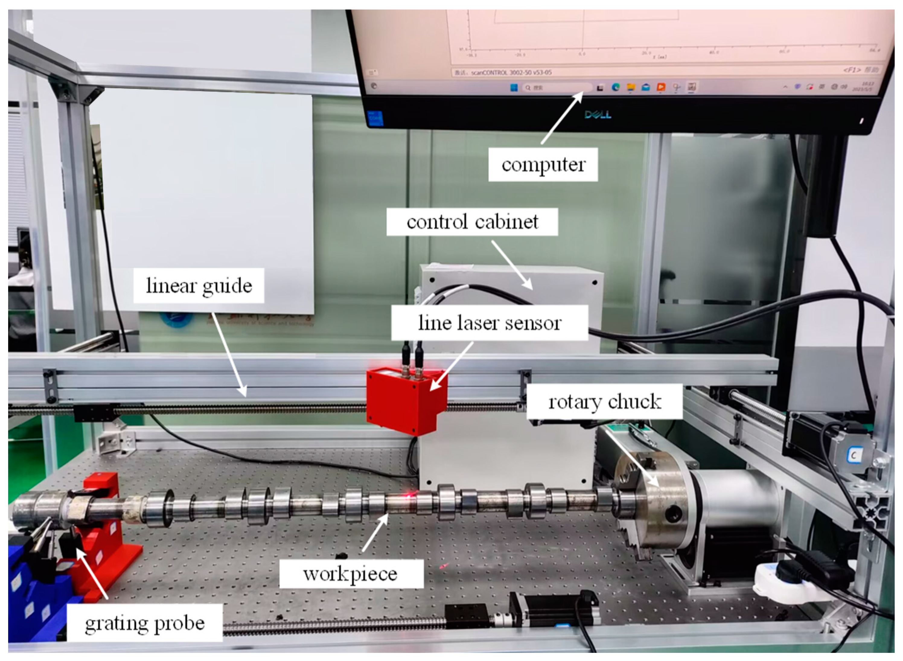
3.1. Experimental Device

In this experiment, the digital grating probe is selected, the model is 7130-10, the baud rate is 9600, and the absolute coded grating can still save the last measurement data after power failure. Digital signal output is adopted, so there is no need to match an amplifier. The measuring range of the probe is 0–12.7 mm, the accuracy is 1.6 μm, the resolution is 0.1 μm, the lateral outgoing line is 0.5 μm, and the force is 1.5 N.

The line laser sensor is a laser profile scanner from Micro-Epsilon Company, Ortenburg, Germany. The model is 3002-50. The measuring range is 50 mm, and it has high resolution in the X-axis and Z-axis directions, which can realize accurate profile measurements. The measuring frequency is up to 10 kHz, which can realize dynamic detection and provide the highest measuring calibration data of 7.37 million points per second. The starting point and ending point of the standard measuring range of the Z axis are 105 mm, the measuring range height is 40 mm, the midpoint is 125 mm, the maximum deviation of a single point is 0.08%, and the linearity of the contour line is 3 μm. The standard measuring range of the X axis starts at 43.3 mm and ends at 56.5 mm, the measuring range midpoint is 50 mm, and the resolution is 2048 points per profile.

As shown in Figure 12, the experimental platform is mainly divided into a clamping device and a measuring device.

The clamping device consists of a chuck and a thimble. One end of the workpiece to be tested is fixed on the rotary chuck, and the other end is fixed by the thimble. The control cabinet is responsible for controlling the rotation of the chuck and its rotating speed so that the workpiece can be scanned all around.

The six grating probes are displaced in the same plane, and the detection plane intersects with the left end face of the workpiece. The line laser sensor is fixed on the linear guide rail of the lead screw and can move back and forth along the guide rail with the slider, and the laser light band irradiates the surface of the workpiece.

Before the measuring system starts measuring, it should be calibrated according to the calibration method described in Section 2. The grating probes are numbered and named in the software system. The experimental data include data collected by a line laser sensor and the data collected by digital grating probes. In order to meet the experimental requirements, the experimental platform was built.

The measured workpiece is a camshaft, for example, which is a typical SW. The camshaft is tested, and the corresponding error parameters are obtained and compared with the measured values of CMM to verify whether it meets the actual requirements. The camshaft for detection is shown in Figure 13.

Fix the grating probe measuring system on the end face of a cylinder with a radius of 30 mm at one end. Record the detection data of the grating probe, calculate the elliptical cross-section data, and then obtain the spatial axis equation so as to determine the position of the spatial camshaft. The surface data of the axis are detected by the line laser sensor, and the data are substituted into the measuring coordinate system to obtain the spatial coordinates of the detection point. When the detection surface is a cylindrical surface, theoretically, the distance from the detection point to the spatial axis to be solved should be a certain value, which is the radius of the cylinder. The application of this method can not only verify the accuracy of the detection system but also calculate the radial circular runout error term by using the detected spatial data and verify the correctness of the algorithm by comparing it with the measurement results of CMM.

The data of six measuring points detected by the operating system through the positioning and measuring mechanism composed of a grating probe are shown in

Table 1. Measured values and coordinates of six grating probes.

Number	1	2	3	4	5	6
Angle/°	15	40	75	70	35	12
Actual value/mm	7.6262	8.1061	8.1002	8.4614	9.3362	9.7081
X coordinate	0	0	0	0	0	0
Y coordinate	−31.9132	−27.1189	−11.3209	8.6604	26.3031	33.5255
Z coordinate	−6.7834	−18.9889	−31.1040	−32.3212	−22.0709	−8.9831

. By subtracting the initial value of the sensor probe from the measured value, the actual change value of the measuring point is obtained. The initial position of the measuring point is known, and the changing coordinate values of X, Y, and Z can be obtained by the distance it moves along a straight line with a known slope, as shown in Table 1.

Through the above points, the ellipse equation of the section is solved by fitting. The coordinate of the center of the ellipse is (0, 1.1276, −1.8054), and the direction vector of the axis is (1.63, −0.59, −0.08), so the equation of the axis is

$$\frac{x}{1.63}=\frac{y-1.1276}{-0.59}=\frac{z+1.8054}{-0.08}$$

(29)

After calibrating the line laser sensor, check the experimental data. It is known that the geometrical surface of the line laser sensor is a cylindrical surface, and the coordinates of the detection point in space can be determined according to the measurement data. The deviation between the calculated point-to-axis distance in the spatial data table and the theoretical value of 30 mm is very small, meeting the experimental requirements.

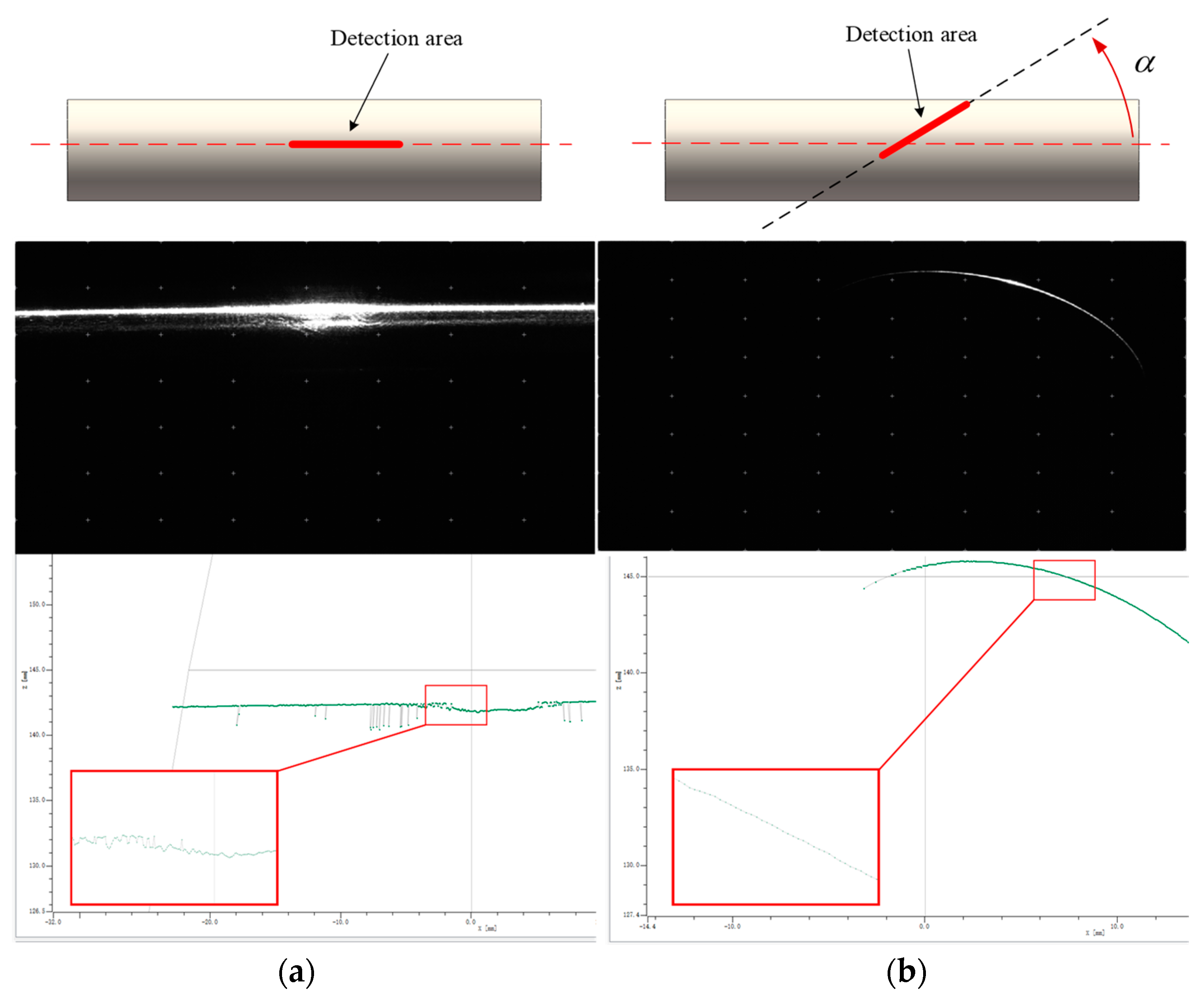
3.2. Results and Discussion

Performs an inspection of a shaft segment on a camshaft. Keeping the line laser sensor still, operate the control cabinet to rotate the chuck. Measure the measurement point data of the same cross-section on the shaft segment several times with the line laser sensor. Process the measurement point data using the radial circular runout characterization method shown in Figure 6. Ten measurements were made on the same cross-section. The test results are shown in

Table 2. Radial circular runout values of ten measurements.

Number	1	2	3	4	5
Radial circular runout/mm	0.3701	0.2393	0.3267	0.4044	0.2651
Number	6	7	8	9	10
Radial circular runout/mm	0.4426	0.3638	0.4416	0.3736	0.4470

.

As can be seen in Table 2, the minimum value of the radial circular runout error of this section is 0.2393 mm, and the maximum value is 0.4470 mm. Therefore, the radial circular runout error of the measured section is 0.4470 mm.

At the same time, the radial circular runout error of the measured section is measured by CMM, and the measurement result shows that the CMM is 0.4401 mm. The results show that the deviation of the experimental results is less than 5% compared with the measurement results of CMM. The accuracy of the detection system is high, as measured by the CMM. The standard deviation of the ten measurements is 0.069 mm. This shows the good repeatability and stability of the detection system.

In the measurement of radial circular runout error, the maximum value is generally selected as the measured value of the item, so it is necessary to pay special attention to the deviation between the measured value of the final radial circular runout and the standard value. It can be found that the experimental results perform well within 5%, while the measured value of other sections is less than the maximum value, and the deviation from the maximum value has no impact on the experimental results.

The experimental results are compared with the radial circular runout tolerance of Figure 1. The radial circular runout tolerance of Figure 1 is generally required to be 0.06 mm, and the experimental measurement result is 0.4470 mm. The main reason for the large difference is the roughness of the surface of the experimental workpiece itself. However, this does not affect the accuracy of the detection system. For CMM, as the current measurement of the highest accuracy of the device, its measurement result as a reference is reasonable.

4. Conclusions

In this paper, a set of online intelligent detection systems for SW is designed, and the overall scheme of the measurement system is also designed. The spatial location algorithm and surface measurement algorithm of the workpiece to be measured are studied. The error compensation and correction are carried out. The hardware platform of the measurement system is built and calibrated, and the detection method is verified by experiments. The surface morphology of the workpiece was measured. The radial circular runout is taken as an example to measure the SSE of the SW. Compared with the traditional measurement results, the deviation of the measurement results is less than 5%.

In this paper, a combination of non-contact measurement and contact measurement is adopted. On the basis of accurately determining the position of the axis, non-contact, all-factor, and online measurement of the workpiece surface can be realized, which conforms to the rapid and informative measurement in the production process of modern enterprises and greatly improves detection efficiency.

References

1. Zhang, S. High-speed 3D shape measurement with structured light methods: A review. Opt. Lasers Eng. 2018, 106, 119–131. [Google Scholar] [CrossRef]
2. Sahoo, S.; Lo, C.Y. Smart manufacturing powered by recent technological advancements: A review. J. Manuf. Syst. 2022, 64, 236–250. [Google Scholar] [CrossRef]
3. Javaid, M.; Haleem, A.; Singh, R.P.; Suman, R. Enabling flexible manufacturing system (FMS) through the applications of industry 4.0 technologies. Internet Things Cyber-Phys. Syst. 2022, 2, 49–62. [Google Scholar] [CrossRef]
4. Yan, R.J.; Kayacan, E.; Chen, I.M.; Tiong, L.K.; Wu, J. QuicaBot: Quality inspection and assessment robot. IEEE Trans. Autom. Sci. Eng. 2018, 16, 506–517. [Google Scholar] [CrossRef]
5. Weimer, D.; Luepke, H.V.; Tausendfreund, A.; Bergmann, R.B.; Goch, G.; Scholz-Reiter, B. Dimensional In Situ Shape and Surface Inspection of Metallic Micro Components in Micro Bulk Manufacturing. Adv. Mater. Res. 2014, 1018, 493–500. [Google Scholar] [CrossRef]
6. Wang, J.; Guo, J. Algorithm for detecting volumetric geometric accuracy of NC machine tool by laser tracker. Chin. J. Mech. Eng. 2013, 26, 166–175. [Google Scholar] [CrossRef]
7. Sang, Y.; Wang, X.; Sun, W. Research on the development of an interactive three coordinate measuring machine simulation platform. Comput. Appl. Eng. Educ. 2018, 26, 1173–1185. [Google Scholar] [CrossRef]
8. Yang, G.; Chen, Y.; Shi, P.; Wang, Y. A three-dimensional measuring system with stroboscopic laser grating fringe. Optik 2021, 229, 166239. [Google Scholar] [CrossRef]
9. Zhao, X.M.; Feng, Y. Measurement method for the symmetry error of double keyway in a shaft. In Proceedings of the 2010 International Conference on Electrical and Control Engineering, Wuhan, China, 25–27 June 2010; IEEE: Piscataway, NJ, USA, 2010; pp. 1257–1259. [Google Scholar]
10. Lim, Y.S.; Choi, W.; Park, Y.J.; Oh, S.W.; Kim, Y.H.; Park, J.S. A novel one-body dual laser profile based vibration compensation in 3D scanning. Measurement 2018, 130, 455–466. [Google Scholar] [CrossRef]
11. Wang, X.; Zhou, Y. A mechanical transmission based image de-blurring method used for on-line surface quality inspection. Measurement 2020, 151, 107262. [Google Scholar] [CrossRef]
12. Leo, M.; Masatoshi, I. Real-Time Inspection of Rod Straightness and Appearance by Non-Telecentric Camera Array. Jrobomech 2022, 34, 975–984. [Google Scholar]
13. Umetsu, K.; Furutnani, R.; Osawa, S.; Takatsuji, T.; Kurosawa, T. Geometric calibration of a coordinate measuring machine using a laser tracking system. Meas. Sci. Technol. 2005, 16, 2466. [Google Scholar] [CrossRef]
14. Guardiani, E.; Morabito, A. An investigation on methods for axis detection of high-density generic axially symmetric mechanical surfaces for automatic geometric inspection. J. Mech. Eng. Sci. 2021, 235, 920–933. [Google Scholar] [CrossRef]
15. Lee, K.H.; Park, H. Automated inspection planning of free-form shape parts by laser scanning. Robot. Comput. Integr. Manuf. 2000, 16, 201–210. [Google Scholar] [CrossRef]
16. Karthikeyan, S.; Subbarayan, M.R.; Beemaraj, R.K.; Sivakandhan, C. Computer vision-based surface roughness measurement using artificial neural network. Mater. Today Proc. 2022, 60, 1325–1328. [Google Scholar]
17. Choi, J.G.; Kim, S. Parallelism Measurement of Rolls by Using a Laser Interferometer. J. Korean Soc. Manuf. Technol. Eng. 2014, 23, 642–646. [Google Scholar] [CrossRef]
18. Angelo, L.; Stefano, P.; Morabito, E.A. Comparison of methods for axis detection of high-density acquired axially-symmetric surfaces. Int. J. Interact. Des. Manuf. 2014, 8, 199–208. [Google Scholar] [CrossRef]
19. Liu, Y.L.; Li, G.C.; Zhou, H.G.; Feng, F.; Ge, W. On-machine measurement method for the geometric error of shafts with a large ratio of length to diameter. Measurement 2021, 176, 109194. [Google Scholar] [CrossRef]
Figure 1. Schematic diagram of measurement elements for SSE of SW.
Applsci 13 12931 g001
Figure 2. Laser triangle detection method.
Applsci 13 12931 g002
Figure 3. Schematic diagram and detection image of the initial position and rotated position of the line laser sensor. (a) The measurement effect when the sensor is not rotating; (b) The measurement effect after the sensor is rotated.
Applsci 13 12931 g003
Figure 4. Schematic diagram of measuring system. (a) The overall view of the system is used to show the overall layout of the device; (b) The layout view of the grating probe detection device shows the specific space layout of the probe.
Applsci 13 12931 g004
Figure 5. Translation and rotation of spatial coordinate system.
Applsci 13 12931 g005
Figure 6. Characterization of radial circular runout.
Applsci 13 12931 g006
Figure 7. Radial installation error.
Applsci 13 12931 g007
Figure 8. Circumferential installation error.
Applsci 13 12931 g008
Figure 9. Axial installation error.
Applsci 13 12931 g009
Figure 10. Schematic diagram of deviation influence. (a) When one measuring point is deviated; (b) When three consecutive measuring points are offset.
Applsci 13 12931 g010
Figure 11. Calibration diagram. (a) XOZ plane; (b) XOY plane.
Applsci 13 12931 g011
Figure 12. Experimental platform.
Applsci 13 12931 g012
Figure 13. Diagram of the measured workpiece.
Applsci 13 12931 g013